Continuous Sensors

A sensor element measures a process variable: flow rate, temperature, pressure, level, pH, density, composition, etc. Much of the time, the measurement is inferred from a second variable: flow and level are often computed from pressure measurements, composition from temperature measurements. A transducer is a device that receives a signal and retransmits it in a different form. For example, we've discussed or we will discuss I/P transducers that convert a current signal to pneumatic form. Most industrial sensors act to detect process variables in the form of a position or voltage change, and hence most sensors also function as transducers. For example, a thermocouple represents a temperature change as a voltage change, while a displacer represents a level change as a change in position of a rotating element. If the sensor element does not produce a signal suitable for transmission through the plant, an additional transducer element is needed. This combined sensor/transducer device is typically called a transmitter, at least in industrial settings. Laboratory equipment manufacturers are likely to refer to the combined device as a transducer.

Continuous Sensors

Continuous sensors convert physical phenomena to measurable signals, typically voltages or currents. Consider a simple temperature measuring device, there will be an increase in output voltage proportional to a temperature rise. A computer could measure the voltage, and convert it to a temperature. The basic physical phenomena typically measured with sensors include;

Angular or linear position Acceleration Temperature Pressure or flow rates Stress, strain or force Light intensity Sound

Most of these sensors are based on subtle electrical properties of materials and devices. As a result the signals often require signal conditioners. These are often amplifiers that boost currents and voltages to larger voltages.

Sensors are also called transducers. This is because they convert input phenomena to an output in a different form. This transformation relies upon a manufactured device with limitations and imperfection. As a result sensor limitations are often characterized with;

Accuracy - This is the maximum difference between the indicated and actual reading. For example, if a sensor reads a force of 100N with a ±1% accuracy, then the force could be anywhere from 99N to 101N.

Resolution - Used for systems that step through readings. This is the smallest increment that the sensor can detect; this may also be incorporated into the accuracy value. For example if a sensor measures up to 10 inches of linear displacements, and it outputs a number between 0 and 100, then the resolution of the device is 0.1 inches.

Repeatability - When a single sensor condition is made and repeated, there will be a small variation for that particular reading. If we take a statistical range for repeated readings (e.g., ±3 standard deviations) this will be the repeatability. For example, if a flow rate sensor has a repeatability of 0.5cfm, readings for an actual flow of 100cfm should rarely be outside 99.5cfm to 100.5cfm.

Linearity - In a linear sensor the input phenomenon has a linear relationship with the output signal. In most sensors this is a desirable feature. When the relationship is not linear, the conversion from the sensor output (e.g., voltage) to a calculated quantity (e.g., force) becomes more complex.

Precision - This considers accuracy, resolution and repeatability or one device relative to another.

Range - Natural limits for the sensor. For example, a sensor for reading angular rotation may only rotate 200 degrees.

Dynamic Response - The frequency range for regular operation of the sensor. Typically sensors will have an upper operation frequency; occasionally there will be lower frequency limits. For example, our ears hear best between 10Hz and 16 KHz.

Environmental - Sensors all have some limitations over factors such as temperature, humidity, dirt/oil, corrosives and pressures. For example many sensors will work in relative humidities (RH) from 10% to 80%.

Calibration - When manufactured or installed, many sensors will need some calibration to determine or set the relationship between the input phenomena, and output. For example, a temperature reading sensor may need to be zeroed or adjusted so that the measured temperature matches the actual temperature. This may require special equipment, and need to be performed frequently.

Cost - Generally more precision costs more. Some sensors are very inexpensive, but the signal conditioning equipment costs are significant.

Industrial Sensors

This section describes sensors that will be of use for industrial measurements. The sections have been divided by the phenomena to be measured.

Angular Displacement Sensors

Potentiometers

Potentiometers measure the angular position of a shaft using a variable resistor. A potentiometer is shown in Figure 14.1. The potentiometer is like a resistor, normally made with a thin film of resistive material. A wiper can be moved along the surface of the resistive film. As the wiper moves toward one end there will be a change in resistance proportional to the distance moved. If a voltage is applied across the resistor, the voltage at the wiper interpolates the voltages at the ends of the resistor.

Potentiometers measure absolute position, and they are calibrated by rotating them in their mounting brackets, and then tightening them in place. The range of rotation is normally limited to less than 360 degrees or

multiples of 360 degrees. Some potentiometers can rotate without limits, and the wiper will jump from one end of the resistor to the other.

Faults in potentiometers can be detected by designing the potentiometer to never reach the ends of the range of motion. If an output voltage from the potentiometer ever reaches either end of the range, then a problem has occurred, and the machine can be shut down. Two examples of problems that might cause this are wires that fall off, or the potentiometer rotates in its mounting.

Encoders

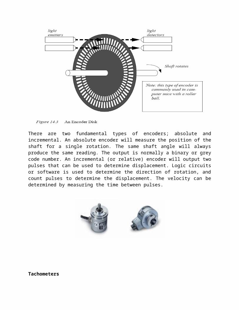
Encoders use rotating disks with optical windows, as shown in Figure 14.3. The encoder contains an optical disk with fine windows etched into it. Light from emitters passes through the openings in the disk to detectors. As the encoder shaft is rotated, the light beams are broken. The encoder shown here is a quadrature encode.

There are two fundamental types of encoders; absolute and incremental. An absolute encoder will measure the position of the shaft for a single rotation. The same shaft angle will always produce the same reading. The output is normally a binary or grey code number. An incremental (or relative) encoder will output two pulses that can be used to determine displacement. Logic circuits or software is used to determine the direction of rotation, and count pulses to determine the displacement. The velocity can be determined by measuring the time between pulses.

Tachometers

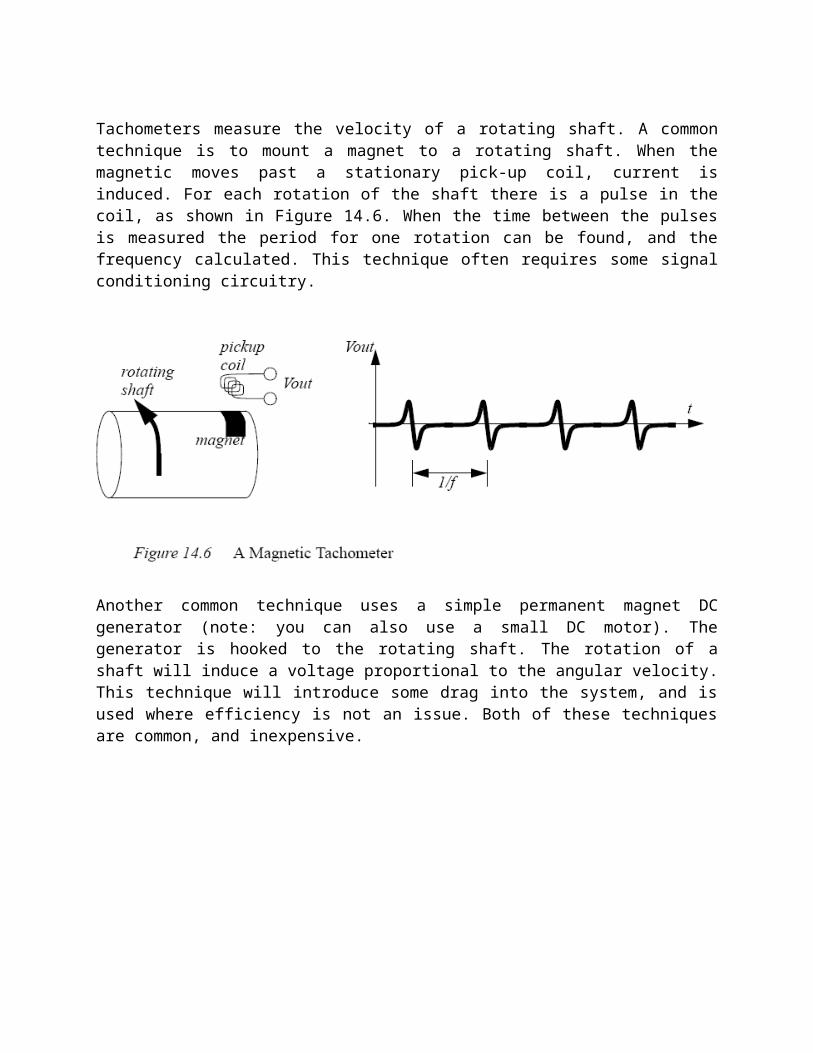
Tachometers measure the velocity of a rotating shaft. A common technique is to mount a magnet to a rotating shaft. When the magnetic moves past a stationary pick-up coil, current is induced. For each rotation of the shaft there is a pulse in the coil, as shown in Figure 14.6. When the time between the pulses is measured the period for one rotation can be found, and the frequency calculated. This technique often requires some signal conditioning circuitry.

Another common technique uses a simple permanent magnet DC generator (note: you can also use a small DC motor). The generator is hooked to the rotating shaft. The rotation of a shaft will induce a voltage proportional to the angular velocity. This technique will introduce some drag into the system, and is used where efficiency is not an issue. Both of these techniques are common, and inexpensive.

Linear Position Sensors

Potentiometers

Rotational potentiometers were discussed before, but potentiometers are also available in linear/sliding form. These are capable of measuring linear displacement over long distances. Figure 14.7 shows the output voltage when using the potentiometer as a voltage divider.

Linear/sliding potentiometers have the same general advantages and disadvantages of rotating potentiometers.

Linear Variable Differential Transformers (LVDT)

Linear Variable Differential Transformers (LVDTs) measure linear displacements over a limited range. The basic device is shown in Figure 14.8. It consists of outer coils with an inner moving magnetic core. High frequency alternating current (AC) is applied to the center coil. This generates a magnetic field that induces a current in the two outside coils. The core will pull the magnetic field towards it, so in the figure more current will be induced in the left hand coil. The outside coils are wound in opposite directions so that when the core is in the center the induced currents cancel, and the signal out is zero (0Vac). The magnitude of the signal out voltage on either line indicates the position of the core. Near the center of motion the change in voltage is proportional to the displacement. But, further from the center the relationship becomes nonlinear.

These devices are more accurate than linear potentiometers, and have less friction. Typical applications for these devices include measuring dimensions on parts for quality control. They are often used for pressure measurements with Bourdon tubes and bellows/ diaphragms. A major disadvantage of these sensors is the high cost, often in the thousands.

Accelerometers

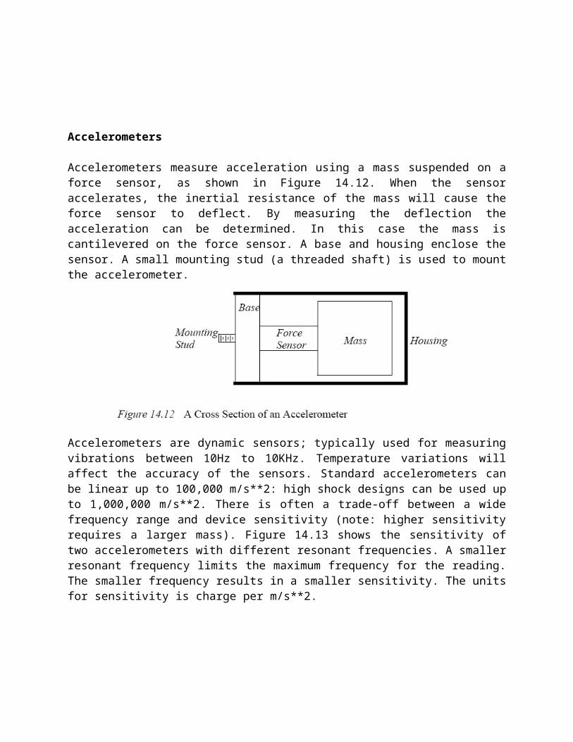
Accelerometers measure acceleration using a mass suspended on a force sensor, as shown in Figure 14.12. When the sensor accelerates, the inertial resistance of the mass will cause the force sensor to deflect. By measuring the deflection the acceleration can be determined. In this case the mass is cantilevered on the force sensor. A base and housing enclose the sensor. A small mounting stud (a threaded shaft) is used to mount the accelerometer.

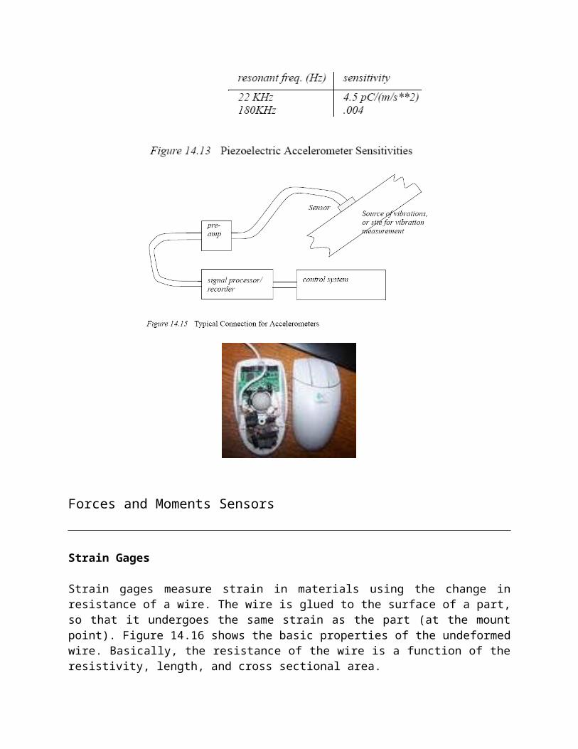
Accelerometers are dynamic sensors; typically used for measuring vibrations between 10Hz to 10KHz. Temperature variations will affect the accuracy of the sensors. Standard accelerometers can be linear up to 100,000 m/s**2: high shock designs can be used up to 1,000,000 m/s**2. There is often a trade-off between a wide frequency range and device sensitivity (note: higher sensitivity requires a larger mass). Figure 14.13 shows the sensitivity of two accelerometers with different resonant frequencies. A smaller resonant frequency limits the maximum frequency for the reading. The smaller frequency results in a smaller sensitivity. The units for sensitivity is charge per m/s**2.

Forces and Moments Sensors

Strain Gages

Strain gages measure strain in materials using the change in resistance of a wire. The wire is glued to the surface of a part, so that it undergoes the same strain as the part (at the mount point). Figure 14.16 shows the basic properties of the undeformed wire. Basically, the resistance of the wire is a function of the resistivity, length, and cross sectional area.

After the wire in Figure 14.16 has been deformed it will take on the new dimensions and resistance shown in Figure 14.17. If a force is applied as shown, the wire will become longer, as predicted by Young’s modulus. But, the cross sectional area will decrease, as predicted by Poison’s ratio. The new length and cross sectional area can then be used to find a new resistance.

Piezoelectric

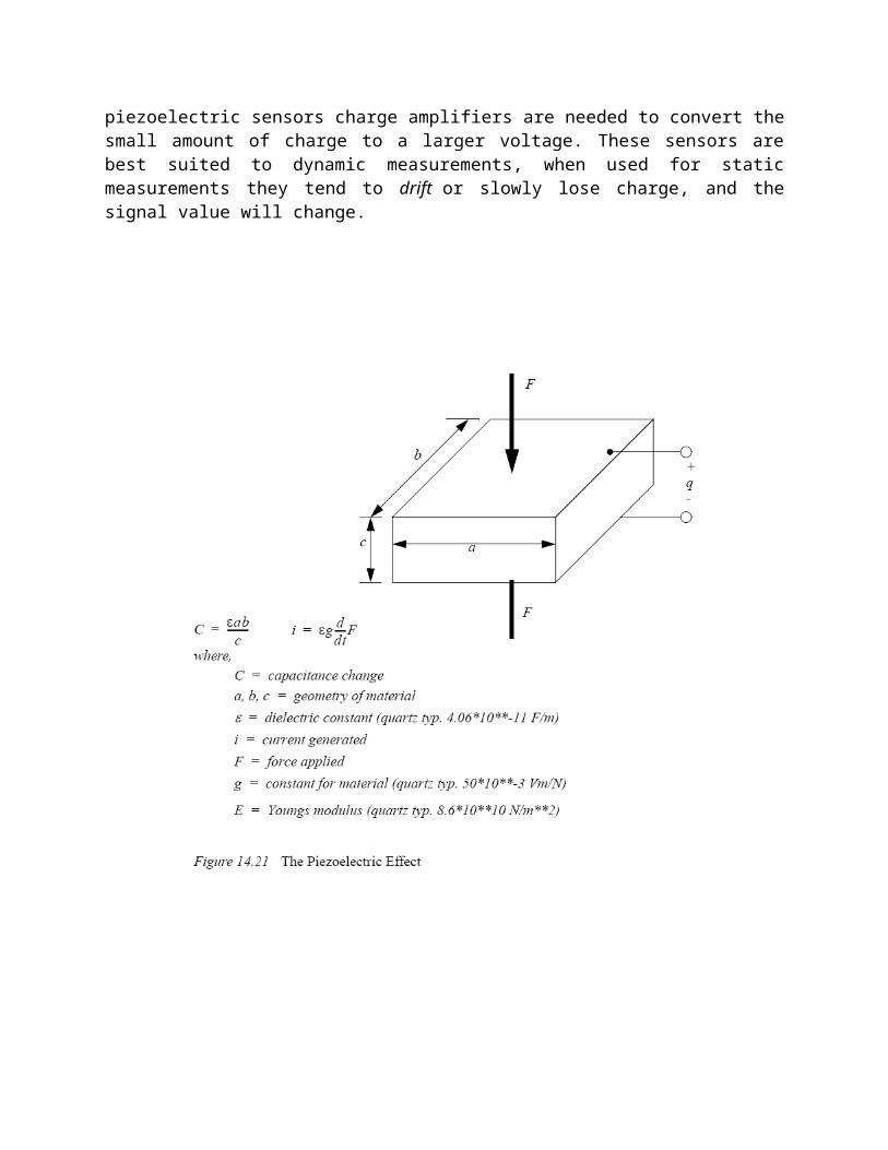
When a crystal undergoes strain it displaces a small amount of charge. In other words, when the distance between atoms in the crystal lattice changes some electrons are forced out or drawn in. This also changes the capacitance of the crystal. This is known as the Piezoelectric effect. Figure 14.21 shows the relationships for a crystal undergoing a linear deformation. The charge generated is a function of the force applied, the strain in the material, and a constant specific to the material. The change in capacitance is proportional to the change in the thickness.

These crystals are used for force sensors, but they are also used for applications such as microphones and pressure sensors. Applying an electrical charge can induce strain, allowing them to be used as actuators, such as audio speakers. When using piezoelectric sensors charge amplifiers are needed to convert the small amount of charge to a larger voltage. These sensors are best suited to dynamic measurements, when used for static measurements they tend to drift or slowly lose charge, and the signal value will change.

http://www.google.co.zm/imgres?imgurl=http://www.imagesco.com/articles/piezo/piezo00.jpg&imgrefurl=http://www.imagesco.com/articles/piezo/piezo00.html&h=408&w=400&sz=22&tbnid=RQPMSPi0wbexSM:&tbnh=227&tbnw=222&prev=/images?q=Picture+of+Piezoelectric&hl=en&usg=__7NTsB8D_ksaxykUXRs7sgALG4D8=&sa=X&ei=NpAsTIisLMHflgfyrd29Cg&ved=0CAkQ9QEwAA

Liquids and Gases Sensors

There are a number of factors to be considered when examining liquids and gasses.

Flow velocity Density Viscosity Pressure

There are a number of differences factors to be considered when dealing with fluids and gases. Normally a fluid is considered incompressible, while a gas normally follows the ideal gas law. Also, given sufficiently high enough temperatures, or low enough pressures a fluid can be come a gas.

When flowing, the flow may be smooth, or laminar. In case of high flow rates or unrestricted flow, turbulence may result. The Reynold’s number is used to determine the transition to turbulence. The equation below is for calculation the Reynold’s number for fluid flow in a pipe. A value below 2000 will result in laminar flow. At a value of about 3000 the fluid flow will become uneven. At a value between 7000 and 8000 the flow will become turbulent.

Pressure

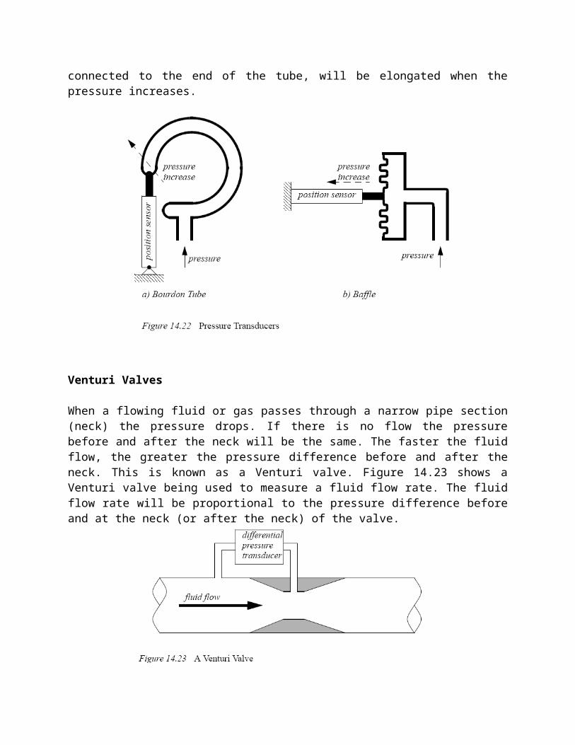
Figure 14.22 shows different two mechanisms for pressure measurement. The Bourdon tube uses a circular pressure tube. When the pressure inside is higher than the surrounding air pressure (14.7psi approx.) the tube will straighten. A position sensor, connected to the end of the tube, will be elongated when the pressure increases.

Venturi Valves

When a flowing fluid or gas passes through a narrow pipe section (neck) the pressure drops. If there is no flow the pressure before and after the neck will be the same. The faster the fluid flow, the greater the pressure difference before and after the neck. This is known as a Venturi valve. Figure 14.23 shows a Venturi valve being used to measure a fluid flow rate. The fluid flow rate will be proportional to the pressure difference before and at the neck (or after the neck) of the valve.

Venturi valves allow pressures to be read without moving parts, which makes them very reliable and durable. They work well for both fluids and gases. It is also common to use Venturi valves to generate vacuums for actuators, such as suction cups.

Coriolis Flow Meter

Fluid passes through thin tubes, causing them to vibrate. As the fluid approaches the point of maximum vibration it accelerates. When leaving the point it decelerates. The result is a distributed force that causes a bending moment, and hence twisting of the pipe. The amount of bending is proportional to the velocity of the fluid flow. These devices typically have a large constriction on the flow, and result is significant loses. Some of the devices also use bent tubes to increase the sensitivity, but this also increases the flow resistance. The typical accuracy for a Coriolis flowmeter is 0.1%.

Magnetic Flow Meter

A magnetic sensor applies a magnetic field perpendicular to the flow of a conductive fluid. As the fluid moves, the electrons in the fluid experience an electromotive force. The result is that a potential (voltage) can be measured perpendicular to the direction of the flow and the magnetic field. The higher the flow rate, the greater the voltage. The typical accuracy for these sensors is 0.5%. These flowmeters don’t oppose fluid flow, and so they don’t result in pressure drops.

Ultrasonic Flow Meter

A transmitter emits a high frequency sound at point on a tube. The signal must then pass through the fluid to a detector where it is picked up. If the fluid is flowing in the same direction as the sound it will arrive sooner. If the sound is against the flow it will take longer to arrive. In a transit time flow meter two sounds are used, one traveling forward, and the other in the opposite direction. The difference in travel time for the sounds is used to determine the flow velocity. A doppler flowmeter bounces a soundwave off particle in a flow. If the particle is moving away from the emitter and detector pair, then the detected frequency will be lowered, if it is moving towards them the frequency will be higher. The transmitter and receiver

have a minimal impact on the fluid flow, and therefore don’t result in pressure drops.

Vortex Flow Meter

Fluid flowing past a large (typically flat) obstacle will shed vortices. The frequency of the vortices will be proportional to the flow rate. Measuring the frequency allows an estimate of the flow rate. These sensors tend be low cost and are popular for low accuracy applications.

Positive Displacement Meters

In some cases more precise readings of flow rates and volumes may be required. These can be obtained by using a positive displacement meter. In effect these meters are like pumps run in reverse. As the fluid is pushed through the meter it produces a measurable output, normally on a rotating shaft.

Pitot Tubes

Gas flow rates can be measured using Pitot tubes, as shown in Figure 14.25. These are small tubes that project into a flow. The diameter of the tube is small (typically less than 1/8") so that it doesn’t affect the flow.

Temperature Sensors

Temperature measurements are very common with process control systems. The temperature ranges are normally described with the following classifications:

Very low temperatures <-60 deg C - e.g. superconductors in MRI units Low temperature measurement -60 to 0 deg C - e.g. freezer controls Fine temperature measurements 0 to 100 deg C - e.g. environmental

controls High temperature measurements <3000 deg C - e.g. metal

refining/processing Very high temperatures > 2000 deg C - e.g. plasma systems

Resistive Temperature Detectors (RTDs)

When a metal wire is heated the resistance increases. So, temperature can be measured using the resistance of a wire. Resistive Temperature Detectors (RTDs) normally use a wire or film of platinum, nickel, copper or nickel-iron alloys. The metals are wound or wrapped over an insulator, and covered for protection. The resistances of these alloys are shown in Figure 14.26.

These devices have positive temperature coefficients that cause resistance to increase linearly with temperature. A platinum RTD might have a resistance of 100 ohms at 0C, that will increase by 0.4 ohms/°C. The total resistance of an RTD might double over the temperature range. A current must be passed through the RTD to measure the resistance. (Note: a voltage divider can be used to convert the resistance to a voltage.) The current through the RTD should be kept to a minimum to prevent self heating. These devices are more linear than thermocouples, and can have accuracies of 0.05%. But, they can be expensive

Thermocouples

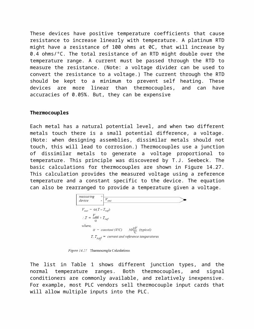
Each metal has a natural potential level, and when two different metals touch there is a small potential difference, a voltage. (Note: when designing assemblies, dissimilar metals should not touch, this will lead to corrosion.) Thermocouples use a junction of dissimilar metals to generate a voltage proportional to temperature. This principle was discovered by T.J. Seebeck. The basic calculations for thermocouples are shown in Figure 14.27. This calculation provides the measured voltage using a reference temperature and a constant specific to the device. The equation can also be rearranged to provide a temperature given a voltage.

The list in Table 1 shows different junction types, and the normal temperature ranges. Both thermocouples, and signal conditioners are commonly available, and relatively inexpensive. For example, most PLC vendors sell thermocouple input cards that will allow multiple inputs into the PLC.

Figure 14.28 Thermocouple Temperature Voltage Relationships (Approximate)

The junction where the thermocouple is connected to the measurement instrument is normally cooled to reduce the thermocouple effects at those junctions. When using a thermocouple for precision measurement, a second thermocouple can be kept at a known temperature for reference. A series of thermocouples connected together in series produces a higher voltage and is called a thermopile. Readings can approach an accuracy of 0.5%.

Thermistors

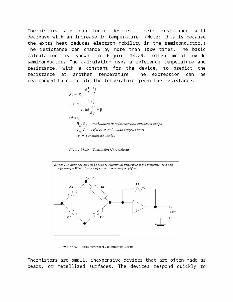
Thermistors are non-linear devices, their resistance will decrease with an increase in temperature. (Note: this is because the extra heat reduces electron mobility in the semiconductor.) The resistance can change by more than 1000 times. The basic calculation is shown in Figure 14.29. often metal oxide semiconductors The calculation uses a reference temperature and resistance, with a constant for the device, to predict the resistance at

another temperature. The expression can be rearranged to calculate the temperature given the resistance.

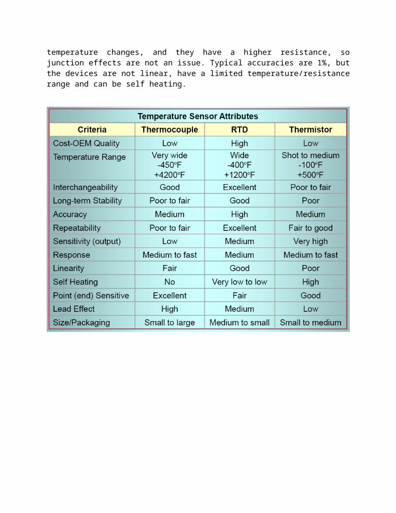
Thermistors are small, inexpensive devices that are often made as beads, or metallized surfaces. The devices respond quickly to temperature changes, and they have a higher resistance, so junction effects are not an issue. Typical accuracies are 1%, but the devices are not linear, have a limited temperature/resistance range and can be self heating.

Light Sensors

Light Dependant Resistors (LDR)

Light Dependant Resistors (LDRs) change from high resistance (>Mohms) in bright light to low resistance (<Kohms) in the dark. The change in resistance is non-linear, and is also relatively slow (ms).

Chemical Sensors

pH

The pH of an ionic fluid can be measured over the range from a strong base (alkaline) with pH=14, to a neutral value, pH=7, to a strong acid, pH=0. These measurements are normally made with electrodes that are in direct contact with the fluids.

Conductivity

Conductivity of a material, often a liquid is often used to detect impurities. This can be measured directly be applying a voltage across two plates submerged in the liquid and measuring the current. High frequency inductive fields are another alternative.