· web viewfilter the data to the year 2017 using the dropdown that appears in cell b1. ... in...

Excel Pivot Tables 2016 Lab Webinar Presenter: Cindy Kredo

File Name: Data File Pivot Tables 3 Hrs.xlsx

Lab 1: Create Simple Pivot Table to Explore the Basics1. Select the tab labeled “Raw Data Start” and explore the data.2. Position the cursor in Cell A2.3. From the Insert Ribbon click the Pivot Table button.4. Confirm the Data Range has been properly identified. The

default placement of the Pivot Table will be on a New Worksheet. Click OK.

5. If necessary, click inside the PivotTable diagram that appears. Doing so will display a Pivot Table Fields dialog box listing each column heading from the data source as a separate field. The Pivot Table Fields dialog box has four boxes on the bottom. The following is a brief description of the purpose of each of these: Filters: Fields added to this box will not be displayed inside the Pivot Table but can be used for

filtering purposes Rows: Fields added to this box will be grouped and displayed vertically in the pivot table: each

group on a separate row. Columns: Fields added to this box will be grouped and displayed horizontally in the pivot table:

each group in a separate column Values: Fields in this box will have math performed on them: sums, counts, etc. All math totals in a

pivot table are based on the entries in this box.6. Add a checkmark to the Department and Amount fields as shown.

By default, checking a text field will drop it into the “Rows Box” at the bottom of the Pivot Table Fields dialog box. Checking numeric fields will drop them into the “Values Box”. Fields can also be dragged into the box of your choice.

7. Do not click the checkmark next to the Year field, but drag and drop the field into the Rows Box.8. Use your mouse to swap the position of the Department and Year fields so that the Year is the first entry

in the Rows Box.

Excel Pivot Tables – Labs 9.30.2017 © Cindy Kredo of 27


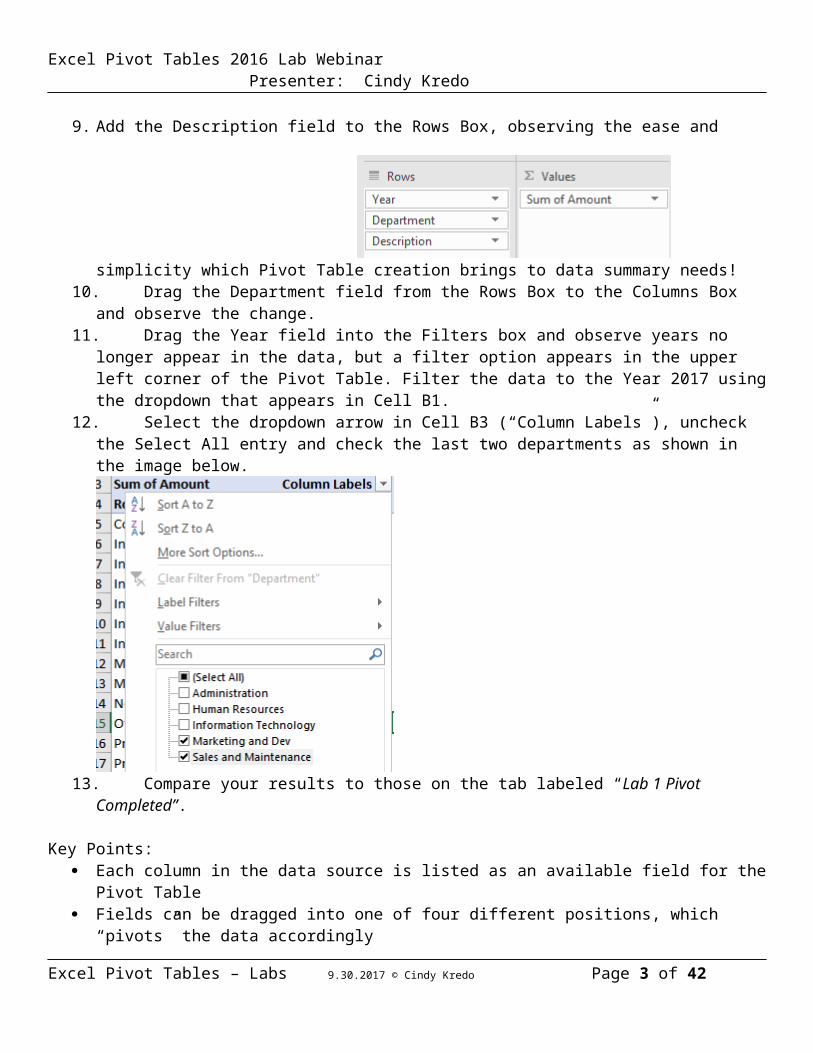
9. Add the Description field to the Rows Box, observing the ease and simplicity which Pivot Table creation brings to data summary needs!

10. Drag the Department field from the Rows Box to the Columns Box and observe the change.11. Drag the Year field into the Filters box and observe years no longer appear in the data, but a filter option

appears in the upper left corner of the Pivot Table. Filter the data to the Year 2017 using the dropdown that appears in Cell B1.

12. Select the dropdown arrow in Cell B3 (“Column Labels”), uncheck the Select All entry and check the last two departments as shown in the image below.

13. Compare your results to those on the tab labeled “Lab 1 Pivot Completed”.

Key Points: Each column in the data source is listed as an available field for the Pivot Table Fields can be dragged into one of four different positions, which “pivots” the data accordingly By default, number fields added to the Values box will be summed Adding a field to the Filters box enables easy filtering of the data, but also removes the display of that

column’s data from the Pivot Table details. Fields in either the Rows box or the Columns box can also be filtered using dropdown arrows in the

Pivot Table data. A small funnel appears to alert the user when filters have been applied. Fields in any one of the four boxes can be removed from the box by (a) right mouse click the field in the

PivotTable Field dialog box and select Remove Field, or (b) drag the field off of the pane


Excel Pivot Tables 2016 Lab Webinar Presenter: Cindy KredoOptional Lab 1: Pivot the Data

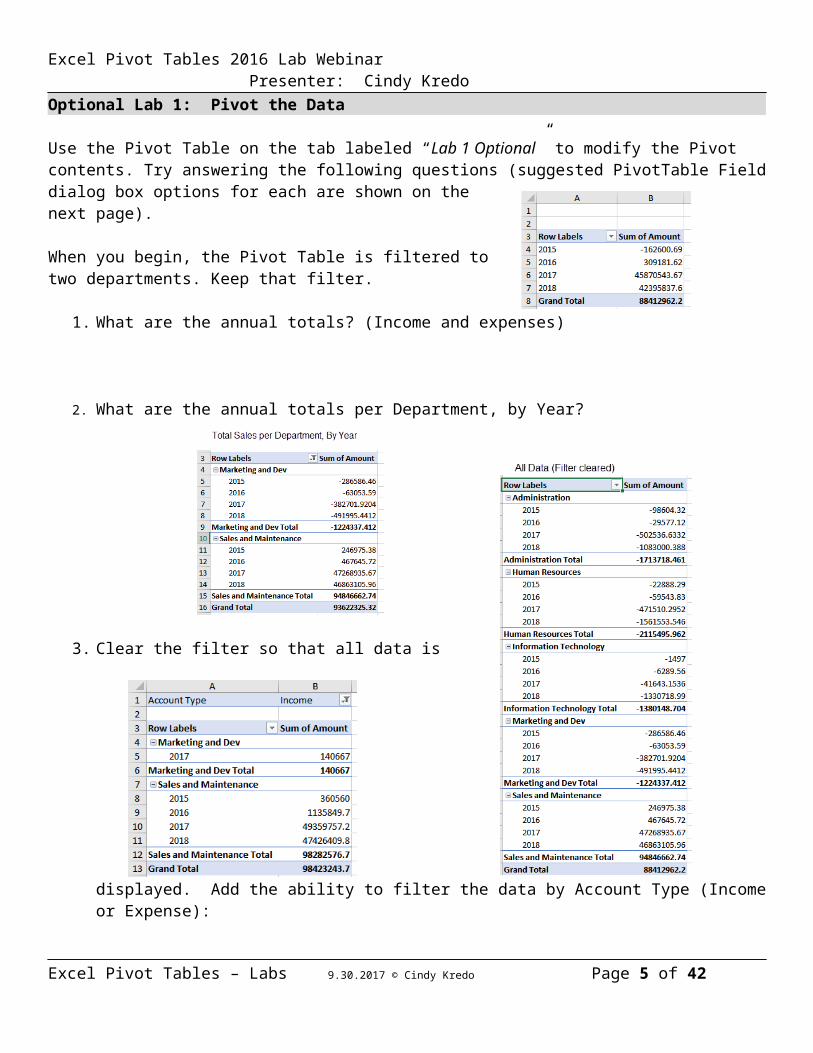
Use the Pivot Table on the tab labeled “Lab 1 Optional” to modify the Pivot contents. Try answering the following questions (suggested PivotTable Field dialog box options for each are shown on the next page).

When you begin, the Pivot Table is filtered to two departments. Keep that filter.

1. What are the annual totals? (Income and expenses)

2. What are the annual totals per Department, by Year?

3. Clear the filter so that all data is displayed. Add the ability to filter the data by Account Type (Income or Expense):

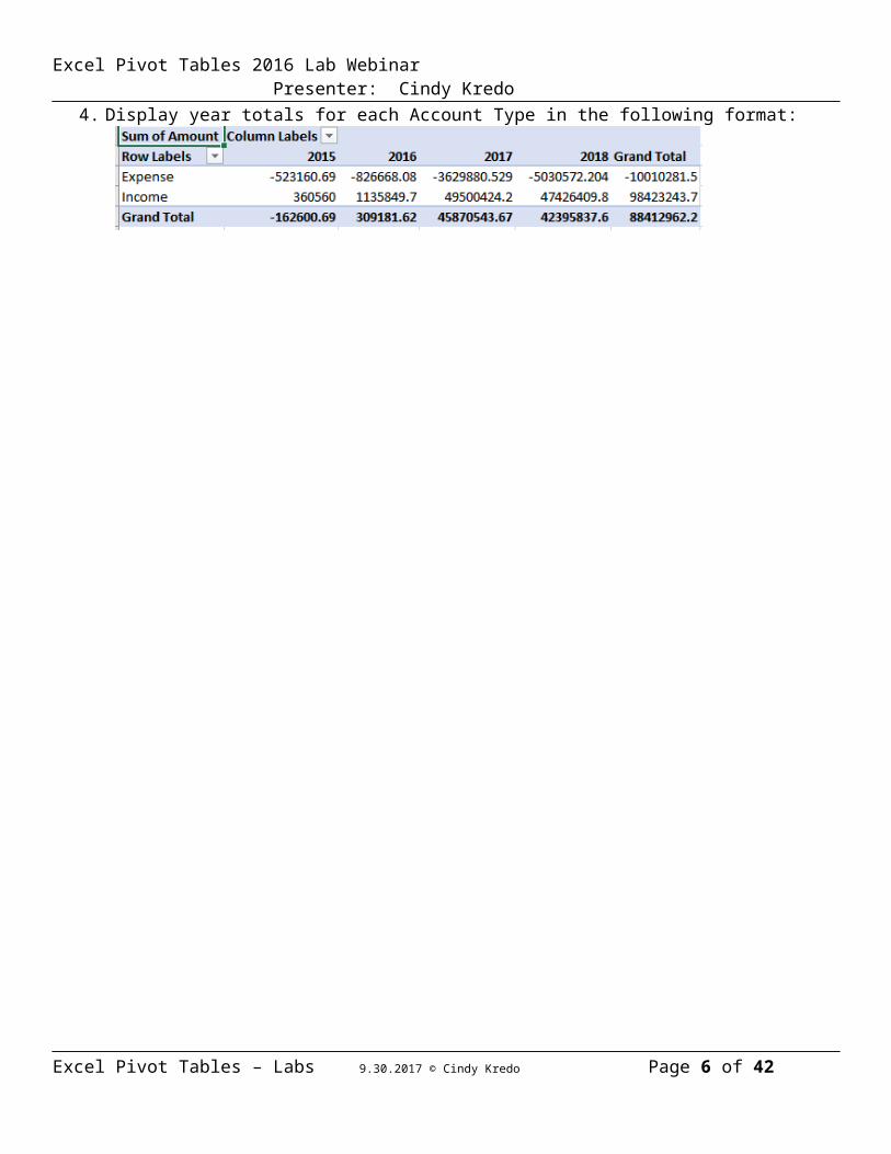
4. Display year totals for each Account Type in the following format:


Excel Pivot Tables 2016 Lab Webinar Presenter: Cindy KredoPivotTable Fields dialog box settings for each of the items on the previous page:

1. 2.

3. 4.

Lab 2: Modify the Pivot

Goal: In this next lab, we will explore the following Pivot Table features:- Report Layout Options and Styles- Changing Number Formats- Sorting- Renaming Labels

1. Review the Pivot Table on the tab labeled “Lab 2-3 Pivot Completed”. This is our end goal. The image along the right side is a sample of the starting point for comparison purposes.

2. Review the Pivot Table on the tab labeled “Lab 2 Start”. In this lab, we will begin modifying this Pivot Table so that it comes closer to the end goal.

3. Compare the placement of the fields that make up the Row box:a. The original Pivot Table shows all Row Items in Column A, whereas the final Pivot Table

displays each Row field in a separate columnb. On the tab labeled “Lab 2-3 Pivot Completed”, click the dropdown arrow in Cell C3 and observe

the filter selections.c. On the lab labeled “Lab 2 Start”, position the

cursor in Cell A5 and use the filter dropdown in Cell A3 to observe the filter selections. Then position the cursor in Cell A6, and once again use the same filter dropdown in Cell A3 to observe the filter selections change.



When more than one field is entered in the Row box, by default Excel will put all fields in Column A. Adding filters to those fields requires proper placement of the cursor before using the dropdown filter box.

4. Change the Report Layout so that all Row fields are displayed in separate columns by using the PivotTable Tools Design Ribbon, Report Layout Button Show in Tabular Form

5. On the PivotTable Tools Design Ribbon, use the PivotTables Styles group to select a PivotTable Style of your choice.

6. Format the numeric values in Column D to have two decimals and a thousands separator:a. Right mouse click any number in the Pivot Tableb. Select Value Field Settings

Click the Number Format button in the left corner of the dialog

c. Select Number, 2 decimals, and thousands separator as shown.


Tip: All Pivot Tables default to Compact Form when first created, which combines all Row fields in the first column. Take a moment to explore the subtle differences between Outline Form and Tabular Form.


TIP: With few exceptions, you are advised to not use the Home Ribbon formatting options or the quick format dialog menu that appears when fields are right-mouse clicked.

Why? Using the Number Format button as shown in Step 6 is the most reliable way to ensure that all numbers in the Pivot Table will retain the same formatting. Other methods can format individual cell addresses instead of the Pivot Table data results.

7. Change the Sort Order of the Account Type field so that Income will appear before Expenses. (Row and Column text data will by default appear sorted alphabetically from A to Z.)

a. Right mouse click the word Expense in Cell B4b. Select Sort Sort Z to A

8. Labels in Pivot Tables can be modified by typing over them. Change the label that reads “Sum of Amount” to read “Totals” by positioning cursor in Cell D3 and typing the word “Totals”. (Existing field names cannot be used. For example, we could not change the words “Sum of Amount” to be “Amount” since Amount is one of the column headings in our raw data.)

9. Save the file – we will continue modifying this Pivot Table in the next lab.


Excel Pivot Tables 2016 Lab Webinar Presenter: Cindy KredoOptional Lab 2: Miscellaneous Useful Tips

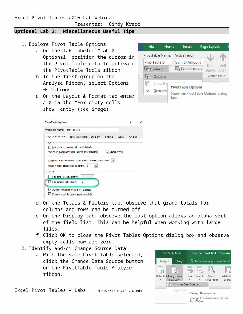
1. Explore Pivot Table Optionsa. On the tab labeled “Lab 2 Optional” position

the cursor in the Pivot Table data to activate the PivotTable Tools ribbon

b. In the first group on the Analyze Ribbon, select Options Options

c. On the Layout & Format tab enter a 0 in the “For empty cells show” entry (see image)

d. On the Totals & Filters tab, observe that grand totals for columns and rows can be turned offe. On the Display tab, observe the last option allows an alpha sort of the field list. This can be

helpful when working with large files.f. Click OK to close the Pivot Tables Options dialog box and observe empty cells now are zero.

2. Identify and/or Change Source Dataa. With the same Pivot Table selected, click the Change

Data Source button on the PivotTable Tools Analyze ribbon.

b. Observe the tab containing the Data Source is now selected, including a dialog box that displays the full range address

c. Click Cancel to return to the Pivot Table.



3. Refresh Pivot Table when Data ChangesWhen changes are made to the source data, Pivot Tables do NOT reflect the change in data unless or until one of the following occurs:a) A user does a right mouse click inside the Pivot Table and selects

Refreshb) The Refresh button is clicked on the PivotTable Tools Analyze Ribbonc) The Pivot Table Options Data Tab Refresh data when opening the

file option is set to yes and the file is re-opened

4. Not sure where to start with Pivot Table ideas?Beginning with Excel 2013, try the Insert Recommended PivotTables button. Try it out on the



Lab 3: Add Splicers

Goal: In this next lab, we will explore Splicers: a dashboard feature that was added to Excel beginning in Version 2010.

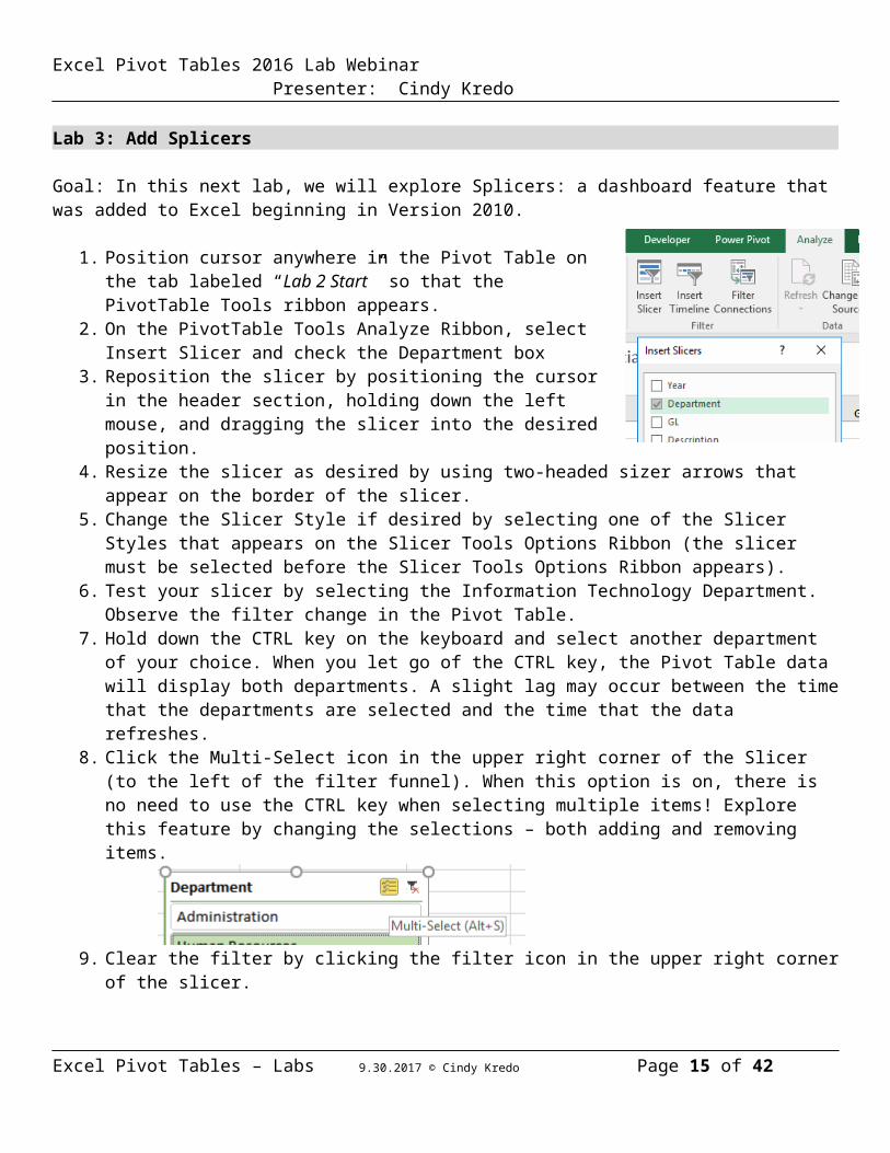
1. Position cursor anywhere in the Pivot Table on the tab labeled “Lab 2 Start” so that the PivotTable Tools ribbon appears.

2. On the PivotTable Tools Analyze Ribbon, select Insert Slicer and check the Department box

3. Reposition the slicer by positioning the cursor in the header section, holding down the left mouse, and dragging the slicer into the desired position.

4. Resize the slicer as desired by using two-headed sizer arrows that appear on the border of the slicer.


Excel Pivot Tables 2016 Lab Webinar Presenter: Cindy Kredo5. Change the Slicer Style if desired by selecting one of the Slicer Styles that appears on the Slicer Tools

Options Ribbon (the slicer must be selected before the Slicer Tools Options Ribbon appears).6. Test your slicer by selecting the Information Technology Department. Observe the filter change in the

Pivot Table.7. Hold down the CTRL key on the keyboard and select another department of your choice. When you let

go of the CTRL key, the Pivot Table data will display both departments. A slight lag may occur between the time that the departments are selected and the time that the data refreshes.

8. Click the Multi-Select icon in the upper right corner of the Slicer (to the left of the filter funnel). When this option is on, there is no need to use the CTRL key when selecting multiple items! Explore this feature by changing the selections – both adding and removing items.

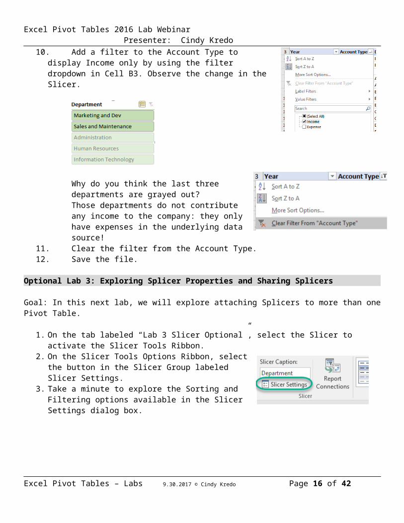
9. Clear the filter by clicking the filter icon in the upper right corner of the slicer.10. Add a filter to the Account Type to display Income only by using the

filter dropdown in Cell B3. Observe the change in the Slicer.

Why do you think the last three departments are grayed out?Those departments do not contribute any income to the company: they only have expenses in the underlying data source!

11. Clear the filter from the Account Type. 12. Save the file.

Optional Lab 3: Exploring Splicer Properties and Sharing Splicers

Goal: In this next lab, we will explore attaching Splicers to more than one Pivot Table.

1. On the tab labeled “Lab 3 Slicer Optional”, select the Slicer to activate the Slicer Tools Ribbon.2. On the Slicer Tools Options Ribbon, select the button in the

Slicer Group labeled Slicer Settings.3. Take a minute to explore the Sorting and Filtering options

available in the Slicer Settings dialog box.



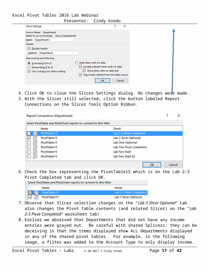
4. Click OK to close the Slicer Settings dialog. No changes were made.5. With the Slicer still selected, click the button labeled Report Connections on the Slicer Tools Option

Ribbon.

6. Check the box representing the PivotTable15 which is on the Lab 2-3 Pivot Completed tab and click OK.

7. Observe that Slicer selection changes on the “Lab 3 Slicer Optional” tab also changes the Pivot Table contents (and related Slicer) on the “Lab 2-3 Pivot Completed” worksheet tab!

8. Earlier we observed that Departments that did not have any income entries were grayed out. Be careful with shared Splicers: they can be deceiving in that the items displayed show ALL departments displayed in any of the shared pivot tables. For example, in the following image, a filter was added to the Account Type to only display income. The numbers that appear do NOT include the Administration, Human Resources, or Information Technology departments, yet those items are not grayed out. That is because the other Pivot Table (located on the tab Lab 2-3 Pivot Completed) DOES include those three departments. Only when both Pivot Tables have had the Income only filter applied would the top three departments appear grayed out.



Lab Four: Date Grouping

GOAL: Explore default Date Grouping

1. Select the tab labeled “Lab 4 Pivot Completed” to observe the end-goal.2. Select the tab labeled “Lab 4 -5 Data” to observe the raw data. A new column, “Post Date” appears in

this data.3. Use the Insert Ribbon to add a Pivot Table to the data. Keep the default settings as displayed to place

your pivot table on a New worksheet



4. Using the Pivot Table Field dialog box that appears on the right, check the square to the left of the Post Date field (in the alternative, the field can be dragged into the Rows box).

Observe that Excel adds Years and Quarters automatically to the Rows box. This is a new feature as of Excel 2013.

5. Drag and drop fields from the top of the list into the boxes on the bottom to match the image displayed on the right

a. Drag Amount into the Values Boxb. Drag Account Type into the Columns Boxc. Drag Department into the Rows Box

6. Position the cursor in Cell A5 and use the PivotTable Tools Analyze Ribbon to click the Expand Field button.

7. Position the cursor in Cell A6 and expand the Qtr1 Entry by using the same Expand Field button.

8. Remove the month grouping by right mouse clicking on any of the date fields select Group deselect the Months option. (By default, Excel Version 2016 will add all three options to most date fields.)



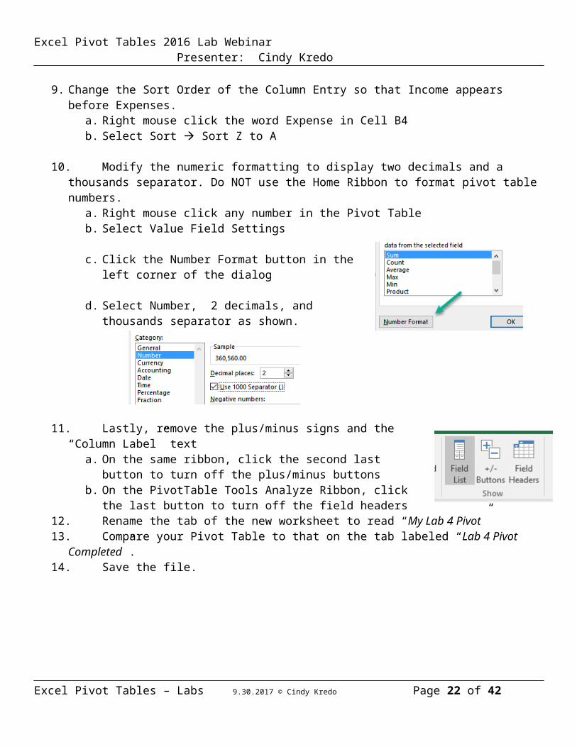
9. Change the Sort Order of the Column Entry so that Income appears before Expenses.a. Right mouse click the word Expense in Cell B4b. Select Sort Sort Z to A

10. Modify the numeric formatting to display two decimals and a thousands separator. Do NOT use the Home Ribbon to format pivot table numbers.

a. Right mouse click any number in the Pivot Tableb. Select Value Field Settings

c. Click the Number Format button in the left corner of the dialog

d. Select Number, 2 decimals, and thousands separator as shown.

11. Lastly, remove the plus/minus signs and the “Column Label” texta. On the same ribbon, click the second last button to turn off the

plus/minus buttonsb. On the PivotTable Tools Analyze Ribbon, click the last button to turn

off the field headers12. Rename the tab of the new worksheet to read “My Lab 4 Pivot”13. Compare your Pivot Table to that on the tab labeled “Lab 4 Pivot Completed”.14. Save the file.



Optional Lab 4: Understanding Grouping and Pivot Caches

When the pivot table was created from the data on the Lab 4-5 Data tab, the Pivot Table Field List contained one entry for each column heading in the original data source.

Whenever grouping is added to a Pivot Table, future Pivot Tables from the same data include the grouped fields created from previous Pivot Tables!

Date fields are not the only type of field that can be grouped, but one must keep in mind that any new groups created will carry into future Pivot Tables.

Is that a good thing? There are advantages – but also potential disadvantages. This optional lab will explore this concept.


Excel Pivot Tables 2016 Lab Webinar Presenter: Cindy Kredo1. Repeat Steps 1 and 2 from Lab 4, starting on the same tab labeled Lab 4-5 Data.2. Drag the Amount Field into the Values Box.3. Drag the Post Date field into the Rows box – observe that Years, Quarters and Post Date appear.4. Right mouse click Cell A4 and select Group5. Deselect the Quarters and Years entries so that the dialog box matches this image:

6. Compare your Pivot Table to the image on the right7. Select the worksheet tab named My Lab 4 Pivot that

was created in the first lab. Observe that you have LOST the original formatting of that Pivot Table!

8. On the worksheet tab named My Lab 4 Pivot, right mouse click a date field and re-select all three date groupings: Months, Quarters and Years.

9. We will now RECREATE the same Pivot Table that was attempted in this Lab, but will do so with a special command that tells Excel to NOT share the Pivot Cache with prior Pivot Tables. How?

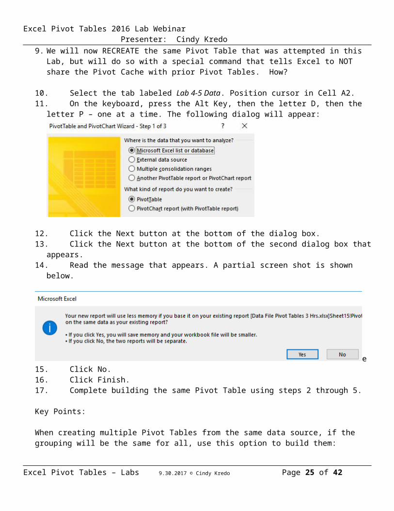
10. Select the tab labeled Lab 4-5 Data. Position cursor in Cell A2.11. On the keyboard, press the Alt Key, then the letter D, then the letter P – one at a time. The following

dialog will appear:

12. Click the Next button at the bottom of the dialog box.


Excel Pivot Tables 2016 Lab Webinar Presenter: Cindy Kredo13. Click the Next button at the bottom of the second dialog box that appears.14. Read the message that appears. A partial screen shot is shown below.

e 15. Click No.16. Click Finish.17. Complete building the same Pivot Table using steps 2 through 5.

Key Points:

When creating multiple Pivot Tables from the same data source, if the grouping will be the same for all, use this option to build them:

If different grouping options will be selected, use the Alt D P method.

The Alt D P method can be added to the QAT toolbar using the Commands Not in the Ribbon category:



Lab 5: Changing the Math / Calculations on More than One Field / Row Group Formatting

Goal: Using the data on the tab labeled “Lab 4-5 Data”, you have been asked to prepare summaries showing the total expenses and average monthly expenses for the four Line Items shown below:

Building Depreciation Building Repairs & Maintenance Equipment Repairs & Maintenance Leased Equipment

In this lab we will change a summary calculation to an average and add a count on another field. We will also explore a formatting selection method that allows for quick formatting across multiple rows for the same grouped item.

1. Navigate to the tab labeled “Lab 4-5 Data” and position the cursor in any one cell below the column headings in preparation for building a Pivot Table.

2. Use the Insert Ribbon to add a new Pivot Table on a new worksheet. Rename the new worksheet tab “My Lab 5.”

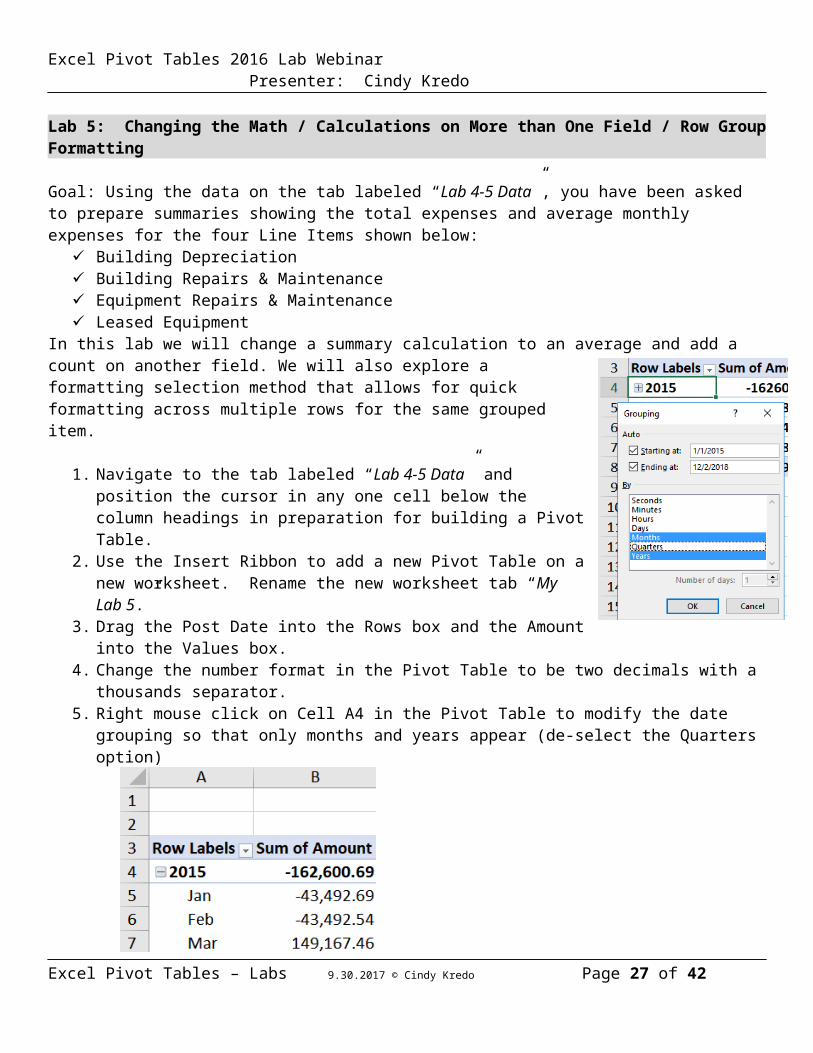
3. Drag the Post Date into the Rows box and the Amount into the Values box.4. Change the number format in the Pivot Table to be two decimals with a

thousands separator.5. Right mouse click on Cell A4 in the Pivot Table to modify the date

grouping so that only months and years appear (de-select the Quarters option)

6. Add a slicer to the Pivot Table using the Description field. (Pivot Table Tools Analyze Ribbon, Insert Slicer, Check Description field). Select the four (Description field) items listed at the beginning of this lab. Tip: The multi-select button in the upper right corner can be used to quickly de-select all: when that is clicked once, the next item selected will de-select all others. Click the multi-select button one more time to then add extra items without needing to hold down the CTRL key!

7. To add the average for each month, drag the Amount field from the top of the PivotTable Fields dialog box into the Values box once again.

8. In the Pivot Table, observe a new Column C has been added with the totals repeated. Right mouse click any one number in Column C and select Summarize Values By Average


Excel Pivot Tables 2016 Lab Webinar Presenter: Cindy Kredo9. Right mouse click any one number in Column C and select Values Field Settings. Use the Number

Format button to change the formatting to be numeric with 0 decimals and a thousands separator.

10. Click the Field Headers button on the PivotTable Tools Analyze Ribbon to hide the words “Row Label” in Cell A3.

11. Change the Labels in Cells B3 and C3 to read “Total” and “Average” as shown

12. After following the above steps, the PivotTable Fields dialog box will match this image

Reposition the fields in the PivotTable dialog box to match the image below and observe the change:



13. Add italic formatting to the Average rows to set them apart from the subtotals. This “grouped row formatting” is the one exception where you can use the popup font dialog box.

a. Click in Cell A6, then position cursor to the left of the word Average in Cell A6 until a small black arrow appears. Click the left mouse button one time: observe all averages are now selected.

b. Right click and use the popup format box to select Italics

TIP: If the small black arrow does not appear, use the Analyze Ribbon, Select Enable Selection option to turn on that setting.

14. Drag the GL field into the Values box. Change the label reading “Count of GL” by typing over the label in Cell A7 to read “Line Item Count”

15. Save the file.

Key Points: - Any numeric field entered in the Values box can be summed, averaged, counted, or multiplied. In

addition, the maximum value or minimum value can be displayed. How?

a) Right mouse click any numeric total in the Pivot Table results Summarize Values By choose calculation type, or

b) In the Values box on the PivotTables Fields dialog box, select the dropdown arrow for the field to be changed Value Field Settings, and choose the type of calculation in the list that appears.

- When Pivot Tables contain more than one type of calculation, group formatting can be done to one or more of the totals to set them apart. A small black arrow on the left edge of the field value in the Pivot Table indicates the item is ready to be selected via a left mouse click.



Lab 6: Drill downs / Grouped Field Expansion / Practicing Earlier Topics

Goal: This lab will introduce two new topics: drill-downs and field expansion. The lab also provides a chance to practice many of the features covered in previous labs. Instructions for previously covered topics are not always included: reference earlier labs if necessary.

1. Skim the data on the “Lab 6” tab.2. You are going to be stranded on a desert island for one month, and can only take TWO food types

(Column B) with you. You want to know which food type has the highest average amount of calories (Energy Column D) per item.

a. Create a pivot table to support your decision by bringing these fields into the Pivot Table field list as shown. Use the drop-down arrow to the right of the Energy [kcal] field to change the summary type to Average.

b. Change the decimals on the average in your Pivot Table to be 2 decimal places.

c. Sort the results from high calorie to low. Position the cursor on any one of the average values in your pivot table, right click, and select Sort, sort largest to smallest.

d. Name the new worksheet tab “Food Pivot”3. Double-clicking on any numeric value in a Pivot

Table will create a new worksheet listing the items that make up that value! We want to explore which individual foods make up the high calorie entries:

a. Double click Cell B4 to create a worksheet tab of all Food Types of “Fats and Oils”b. Return to the Pivot Table and Double Click Cell B5 to create a worksheet tab of all Food Types

of “Nuts, Seeds and Products”c. Delete the drill-down worksheets if desired.



4. Double-click the grouped label in Cell A5 and observe the popup dialog box:

5. Select the Energy (kcal) item and click OK. Observe this is not a drill-down: it simply expanded the data in the Pivot Table to show the field selected, adding +/- symbols.

Explore the other Food Types, using the +/- symbol to expand or collapse the field, observing that the Energy (calorie) detail is always displayed in the expanded rows.

Remove the grouped field expansion by right clicking on one of the expanded rows as shown in the image.

6. Use the PivotTable Tools Analyze ribbon to select the Expand Field button. Observe this button serves the same purpose: the only difference is that there is no option to remove a selected item.

7. Select Cancel to close the dialog box.8. Add the Food field (Column A) to your pivot table as a row label.

Your Pivot table field list should look like this:

9. Change the report layout of your pivot table to tabular. (How? PivotTable Tools Design Ribbon, Report Layout button)

10. Add the average fiber to the Pivot Table in the Values position and format the new field to display two decimals.

11. Compare your Pivot Table to the image below.



12. Save the file.

Lab 7: Adding Value and Label Filters / Subtotals

Goal: Explore the ability to add filters based on numeric values and/or text values

1. Select the tab labeled “Lab 7 Start” and position the cursor in Cell A4.2. Observe the individual food fiber entries and the average totals within each Food Type.3. Add a filter to this Pivot Table to only display those Food Types where the average fiber is great than 2.

a. Right mouse click on any one of the Food Type items in Column Ab. Select Filter Value Filters from the pop-up menuc. Complete the dialog as shown

4. Observe that individual foods (i.e. English Walnuts) can exceed 2 grams of fiber: our filter was placed at the Food Type level!

5. Remove the fiber subtotal from the Food Type fielda. Right mouse click on any one of the Food Type

items in Column Ab. Remove the check from the Subtotal “Food Type:

entry



6. Add a filter to the Pivot Table to further limit the individual foods in Column B to those where the word “raw” appears.

a. Right click Cell B4 b. Select Filter Label Filters from the pop-up menuc. Complete the dialog as shown.

Value Filters are used to control numeric filtering; Label Filters are used to control text filtering.

7. Further file the pivot table to those Food items (Column B) that excel 100 calories. This is NOT as straightforward as it would seem!

By default, Value Filters and Label Filters cannot be applied to the same field without changing the Pivot Table Options

a. Right mouse click any field in the Pivot Table, select Pivot Table Optionsb. Select the Totals & Filters tabc. Check the box labeled “Allow multiple filters per field”d. Click Ok to close the dialog box e. Right click Cell B4 and add the Value calorie filter as shown:


Excel Pivot Tables 2016 Lab Webinar Presenter: Cindy Kredo8. To see whether Value and/or Label filters have been set on any given field:

a. Right mouse click the group label field: i.e. Cell B3b. Observe checkmarks to the left of the filter types

9. If time permits, clear all Filters from the Food field, turn OFF the multiple field filter option in the Pivot Table options, and repeat steps 6 and 7 WITHOUT changing the multiple field filter option. Observe that after entering the Value Filter, the Label Filter was automatically removed without any prompting.


Excel Pivot Tables 2016 Lab Webinar Presenter: Cindy KredoOptional Lab: Timelines – New to Excel 2016

Timeline filters can now be added to Pivot Tables that include date fields.

After clicking OK, the timeline appears as a dashboard filter.The Pivot Table totals are filtered based on the selected range on the timeline.

Optional Lab: Handling Missing Data

1. Explore the two Pivot Tables on the tab labeled “Optional Display Missing Data”2. To display all years, regardless of whether data exists for that year, right mouse click the field to be

modified and select Field Settings check the box labeled “Show items with no data”3. If desired, change the PivotTable Options to show 0’s in empty cells.


Excel Pivot Tables 2016 Lab Webinar Presenter: Cindy KredoOptional Lab: Pivot Charts / Copying Pivot Tables

1. Explore the tab labeled Optional Pivot Charts.2. Filter the data to Regions A and B using the Filter dropdown arrow in Cell A33. Observe the Pivot Chart automatically took on the same filter4. Remove the filter.5. If you need more than one chart from the same Pivot Table data displaying different filters, copy the

original Pivot Table and create the new chart based on a copy:a. Position cursor in the Pivot Tableb. On the PivotTable Tools Analyze Ribbon use the

button labeled Select Entire PivotTablec. CTRL C to copy the Pivot Tabled. Move to Cell A19 and CTRL V to paste a copy of the

Pivot Tablee. With this Pivot Table still selected, select PivotChart

on the Analyze Ribbon.f. Select a Column Chart.g. Reposition the chart as needed.h. Change the filter in the second Pivot Table to cover

Regions A and B. Observe the first Pivot Table did not change.

Optional Lab: Report Filter Pages

1. Make a copy of the worksheet tab labeled “Lab 1 Pivot Completed” (right mouse click the tab name, select Move or Copy, check the box in the left corner to create a copy and place it in the front of all other tabs.

2. Clear the filter from the Year field so that all years are displayed.3. Observe the Year field is in the Filters box

4. On the PivotTables Tools, Analyze ribbon, select the Options dropdown as shown in the image below Show Report Filter Pages.

5. Observe the copied worksheet tab is no longer the first worksheet tab in the file: separate Pivot Tables for each year were created!

6. This option is only available for fields placed in the Filters box.


· web viewfilter the data to the year 2017 using the dropdown that appears in cell b1. ... in...

Documents