file · web viewdevelopment of a unified land model with multi-criteria observational data for the...
TRANSCRIPT

DEVELOPMENT OF A UNIFIED LAND MODEL WITH MULTI-CRITERIA
OBSERVATIONAL DATA FOR THE SIMULATION OF REGIONAL HYDROLOGY
AND LAND-ATMOSPHERE INTERACTION
Ben Livneh
A dissertation
submitted in partial fulfillment of the
requirements for the degree of
Doctor of Philosophy
University of Washington
2012
Reading Committee:
Dennis P. Lettenmaier, Chair
Pedro J. Restrepo
Erkan Istanbulluoglu
Program Authorized to Offer Degree:
Civil and Environmental Engineering
University of Washington
Abstract
DEVELOPMENT OF A UNIFIED LAND MODEL WITH MULTI-CRITERIA
OBSERVATIONAL DATA FOR THE SIMULATION OF REGIONAL HYDROLOGY
AND LAND-ATMOSPHERE INTERACTION
Ben Livneh
Chair of the Supervisory Committee:
Professor Dennis P. Lettenmaier
Department of Civil and Environmental Engineering
A unified land model (ULM) is described that combines the surface flux parameterizations
in the Noah land surface model (used in most of NOAA’s coupled weather and climate
models) with the Sacramento soil moisture accounting model (Sac; used for hydrologic
prediction within the National Weather Service). The major motivation was to develop a
model that has a history of strong hydrologic performance, while having the ability to be
used as the land surface parameterization in coupled land-atmosphere models. Initial
comparisons were made with observed surface fluxes and soil moisture wherein ULM
performed well compared with its parent models (Noah, Sac) with a notably improved
representation of the soil drying cycle. Parameter tuning was ultimately needed to capture
streamflow dynamics, leading to a parameter estimation framework that utilized multiple
independent data sets over the continental United States. These included a satellite-based
evapotranspiration (ET) product based on MODerate resolution Imaging Spectroradiometer
(MODIS) and Geostationary Operation Environmental Satellites (GOES) imagery, an
atmospheric-water balance based ET estimate that utilizes North American Regional
Reanalysis (NARR) atmospheric fields, terrestrial water storage content (TWSC) data from
the Gravity Recovery and Climate Experiment (GRACE), and streamflow (Q) primarily
ii

from United States Geological Survey (USGS) stream gauges. At large scales (≥ 105 km2)
calibrations using Q as an objective function resulted in the best overall multi-criteria
performance. At small scales (< 104 km2), about one-third of the basins had their highest Q
performance from multi-criteria calibrations (to Q and ET) suggesting that traditional
calibration may benefit by supplementing remote sensing data. Finally, a scheme to transfer
calibrated parameters was employed using Principal Components Analysis (PCA) to derive
predictive relationships between model parameters and commonly used catchment
descriptors (meteorological, geomorphic, land-cover characteristics), several satellite
remote sensing products, as well as the Geospatial Attributes of Gages for Evaluating
Streamflow (GAGES-II) database. Regional model performance was most improved when
locally optimized parameter were first resampled based on their performance at
neighboring basins, termed zonalization. For a large number of basins, the regionalized
model performed comparably to the calibrated version, affirming this PCA methodology as
a viable means for transferring geospatial parameter information.
iii

TABLE OF CONTENTSI. INTRODUCTION..............................................................................................................1
1.1 Science questions......................................................................................................4
II. DEVELOPMENT OF THE UNIFIED LAND MODEL...................................................5
2.1 Introduction...................................................................................................................5
2.2 Model Structure.............................................................................................................8
2.2.1 Noah.......................................................................................................................8
2.2.2 Sac........................................................................................................................10
2.2.3 ULM.....................................................................................................................11
2.3 Model testing and evaluation strategy........................................................................14
2.4 Study areas and data....................................................................................................16
2.4.1 Study basins..........................................................................................................16
2.4.2 Surface fluxes and soil moisture observations.....................................................18
2.5 Model validation and discussion.................................................................................21
2.5.1 Surface fluxes.......................................................................................................21
2.5.2 Soil moisture.........................................................................................................23
2.5.3 Streamflow and parameter sensitivities................................................................25
2.6 Conclusions.................................................................................................................34
Iii. Multi-criteria parameter estimation for the Unified Land Model...................................36
3.1 Introduction.................................................................................................................36
3.2 Modeling context.......................................................................................................37
3.3 Data and Methods.......................................................................................................38
3.3.1 Basin selection, streamflow, and meteorological data.........................................38
3.3.2 Auxiliary model evaluation data..........................................................................41
3.3.3 Land surface model..............................................................................................45
3.3.4 Calibration procedure and error analysis..............................................................46
3.4 Results and Discussion................................................................................................48
3.4.1 Single criterion calibrations..................................................................................48
3.4.2 Multi-criteria calibrations.....................................................................................57
3.4.3 Hydrologic response and model error analysis....................................................62
iv

3.5 Conclusions.................................................................................................................67
IV. Regional parameter estimation for the Unified Land Model..........................................69
4.1 Introduction.................................................................................................................69
4.2 Methods.......................................................................................................................71
4.2.1 Study area and data sources..................................................................................71
4.2.2 Model forcing data...............................................................................................72
4.2.3 Catchment attribute data.......................................................................................72
4.2.4 Land surface model..............................................................................................74
4.2.5 Regionalization procedure....................................................................................75
4.2.6 Principal Components Analysis (PCA)................................................................78
4.3 Results and discussion................................................................................................79
4.3.1 Spatial Coherence.................................................................................................79
4.3.2 Simulated streamflow performance......................................................................82
4.3.3 Principal components and catchment descriptors................................................86
4.3.4 Global parameter estimation experiment.............................................................91
4.4 Summary and conclusions..........................................................................................93
V. CONCLUSIONS.............................................................................................................95
VI. References......................................................................................................................98
v

List of FiguresFigure 2.1: Schematic of the Noah LSM including required forcing variables, evaporative components of transpiration, ET, canopy evaporation, EC, soil evaporation, ES, and snow sublimation, SS. Precipitation is partitioned into evapotranspiration, runoff and infiltration.................................................................................................................................................9Figure 2.2: Schematic of the Sac model, including required forcing variables and evaporative components. The upper zone tension and free water contents (UZTWC and UZFWC, respectively) can vary from 0 to a maximum value (UZTWM and UZFWM, respectively). Similarly, lower zone tension water, primary and secondary free water contents (LZTWC, LZFPC, LZFSC respectively) can also vary from 0 to a maximum value (LZTWM, LZFPM, LZFSM respectively)...........................................................................11Figure 2.3: Schematic of ULM, including required forcing variables, moisture and energy components. Precipitation, P, and snowmelt, SM, are partitioned into direct runoff, RD, infiltration, and evapotranspiration. Infiltration becomes either surface runoff, RS, or interflow, I.F., in the upper zone, the remains of which can then infiltrate further into the lower zone and become baseflow, B. The double arrows represent the transfer of model structure, wherein the soil schematic on the left is only considered for soil moisture computations, while the schematic on the right is used for all other model computations.. 12Figure 2.4: Location of study basins (shaded areas), flux tower sites (black circles), and ICN soil moisture stations (numbered).................................................................................16Figure 2.5: Mean monthly precipitation (right axis, bars) and streamflow (left axis, lines) for the 6 study basins............................................................................................................17Figure 2.6: Scatter plots of observed energy balances (sensible (SH) plus latent (LE) plus ground heat flux (G) versus net radiation (Rnet). Shown on each plot are the slope of the line of best fit (m) and the bias (W/m2), where a slope of m=1, and bias = 0 would characterize zero energy balance closure error. A single summer is shown for each site, namely Blodgett Forest (2004), Niwot Ridge (2006), Brookings (2005), and Howland (2001)....................................................................................................................................20Figure 2.7: Mean diurnal fluxes (W/m2) for ULM during summer for 4 Ameriflux sites shown at 30-minute intervals for the years with greatest energy balance closure at Blodgett Forest (2004), Niwot Ridge (2006), Brookings (2005), and Howland Forest (2001)..........22Figure 2.8: Observed (black circle) volumetric soil moisture, compared with ULMA (red circle) and Noah (blue circle) during the warm season at Blodgett forest (2004) and Niwot Ridge (2006).........................................................................................................................24Figure 2.9: Illinois Climate Network (ICN) soil moisture data in units of millimeters of water equivalent (observations shown in black); where the leftmost 4 plots show the mean monthly soil moisture for the 4 model soil layers of ULM (red), Noah (blue), while the upper right plot shows the entire soil column, including Sac (green), and the lower right plot shows the change in monthly soil moisture for the entire soil column.........................25Figure 2.10: RMSE between simulated and observed streamflow (1960 – 1969) based on 15 parameter values varying uniformly within their plausible range (Table 2.3) plus an additional simulation using the a priori value for that parameter (black circle). Shown are only the most sensitive parameters for each basin based on this method.............................27Figure 2.11: Mean monthly streamflows (1960 – 1969) for ULM using a priori parameters (ULMA), ULM with parameters tuned towards maximized model efficiency (ULMM), Noah, Sac, and observations.................................................................................................28
vi

Figure 2.12: NSE values (multiplied by -1 for consistency with RMSE minimizations) corresponding to simulated versus observed streamflow for variation of individual parameter values following a Monte Carlo approach. For each basin, the scatter-plots of the two most sensitive parameters are shown (lower plots) with the best 4 simulations circled in blue for ease of viewing. The upper plots show trends in the data grouped into 50-simulation-bins, with bin minima in blue showing an envelope of parameter sensitivity and bin means in red. The ADIMP parameter (not shown) was found to be highly sensitive for all basins with an approximate minimum value of 0.225...............................................29Figure 2.13: Daily streamflows and precipitation over the 1964 water year for the ILLIN (a) and BROOK (b) basins. Observed flow (solid black), ULMM (dashed black line), ULMA (dashed orange line), Noah (dashed pink line), and Sac (dashed green line) are included. These two basins provided the greatest challenge in modeling with relatively sporadic precipitation, and sharp streamflow peaks (BROOK: end of March snowmelt and soil thaw streamflow spike was poorly captured by the snow model and frozen soil physics).................................................................................................................................30Figure 3.1: Large-scale study domain, including precipitation gauges (black dots), as well as major hydrologic regions (shaded) that are defined through their drainage at stream gauges (blue circles). The un-shaded areas within these regions are either downstream of the stream gauge, or consist of many smaller river basins which drain directly into the Atlantic or Pacific Oceans or the Gulf of Mexico................................................................39Figure 3.2: Small-scale study domain comprised of 250 tributary catchments using USGS stream gauges that were screened to be minimally affected by diversions, with at least 20 years of data in the past 3 decades to facilitate multicriteria comparisons...........................41Figure 3.3: Example schematic of the Upper Mississippi river basin components needed to perform an atmospheric water balance to estimate ET (equation 3.1), including atmospheric moisture convergence, C, change in precipitable water, dPw/dt, and precipitation, P..........43Figure 3.4: Mean monthly hydrographs in m3/s for the major basins for a 20 year period, the beginning of which varies by basin, depending on data availability..............................49Figure 3.5: Estimates of mean monthly evapotranspiration by an atmospheric water balance (ETAWB – section 2.2.1) in squares, and through satellite data (ETSAT – section 2.2.2) in circles compared with the residual of precipitation, P, minus streamflow, Q, for the major basins and smaller tributaries (smaller circles). Shaded areas denote the domain within which ET was estimated, such that un-shaded circles represent ET from tributaries outside the major basins....................................................................................................................51Figure 3.6: Comparisons of the residual of evapotranspiration from satellite data (ETSAT –section 3.2.2.2) with precipitation, P, minus streamflow, Q, for the major river basins (larger circles) and smaller tributaries (smaller circles) 2001 – 2010, as a function of VI-Ts diversity, expressed as a product of the ranges of NDVI and skin temperature for each basin. Departures from the dashed line denote either an uncertainty in ET estimates, or significant long-term TWS, or other observational errors....................................................52Figure 3.7: Mean monthly ET (mm) for the major river basins for the period 2001 – 2010 that include two sets of calibrations, satellite-based (SAT) or atmospheric water balance-based (AWB) observational products as well as the control simulation..............................54Figure 3.8: Mean monthly TWSC (mm) for the major river basins for the period 2002-2010 including the control and calibrated model simulations; the range of variability for each case is shown accordingly....................................................................................................55
vii

Figure 3.9: NSE values for ULM calibrations to streamflow at a daily time step as a function of AI for the period 1991-2010. Shading of individual points denotes the major region for each tributary.......................................................................................................56Figure 3.10: NSE values for ULM calibrations towards ETSAT at a daily time step as a function of AI for the period 2001-2010. Shading of individual points denotes the major region for each tributary.......................................................................................................57Figure 3.11: ULM calibrations over major basins towards combinations of Q,ETSAT, ETAWB, and TWSC at a monthly time step for the period 1991-2010, including (a) NSE values for each criteria (cutoff at -1 for clarity), and (b) differences in rRMSE for each criteria resulting from the respective calibrations. The entire set of results for these plots is included in Table 3.3 and Table 3.4.....................................................................................58Figure 3.12: ULM calibrations over tributary basins towards combinations of Q, and ETSAT at a daily time step for the period 1991-2010, including (a) NSE values for each criteria and (b) differences in rRMSE for each criteria resulting from the respective calibrations.........62Figure 3.13: Comparison between major basin and mean tributary flows and errors. Flow data was converted to z-scores to allow for comparison among basins. The differences in aridity index (AI) are shaded according to the upper-scale for the top 3 panels and the lower scale for the bottom panel...........................................................................................66Figure 4.1: Map of the study domain, including 220 basins (yellow) and location of precipitation gages used in the forcing data set (fine black dots).........................................72Figure 4.2: Flow chart illustrating the procedure for selecting locally and zonally optimized model parameters based on ranking Nash-Sutcliffe efficiency (NSE) from Pareto-optimal parameter sets that were non-dominant in terms of Pearson correlation, R, difference in means, α, and difference in standard deviation, β................................................................77Figure 4.3: Example illustrating the spatial coherence of a set of candidate inputs for the regionalization experiments, which regionalize predictors (catchment attributes) and predictands (ULM parameters) that were selected either zonally or locally (e.g. Exp. 1 uses local predictands and local predictors as inputs to the PCA regionalization, see Table 4.3 for other experiments). The western U.S. is enlarged to show the spatial coherence of the zonal parameter value, UZTWM..........................................................................................79Figure 4.4: Experimental variograms for both zonal and local model parameters, illustrating greater spatial coherence for zonal parameters shown. Only those parameters with a detectable range are included, which is consistently present for zonal parameters..............81Figure 4.5: Illustration of tradeoffs in model performance when running (a) zonal parameters (θP-ZONAL) locally and (b) running local parameters (θP-LOCAL) zonally (averaged NSE over a 5° latitude-longitude window – see Figure 4.2 for definitions). The solid-black line was drawn connecting ranked Nash-Sutcliffe Efficiency (NSE) for 220 basins and represents the upper-envelope for model performance, either locally (a), or zonally (b), while the thin gray lines show that the penalty in local performance for using θP-ZONAL is much smaller than the penalty in zonal performance using θP-LOCAL....................................83Figure 4.6: Comparison of the four regionalization experiments with local optimizations. The solid black line represents the NSE of each basin (ranked) as in Figure 4.5a, whereas the colored lines show regionalized model skill (ULMR) for each experiment. The first word in the panel labels refers to which parameters, θ, were used, while the second refers to the catchment descriptors, η, such that, for example, “ZONAL-LOCAL” represents the regionalization using zonal model parameters with local catchment descriptors.................85
viii

Figure 4.7: Comparison of ULM using locally optimized parameters with the original regionalization experiments (ULMR, section 4.3.2) and the global experiments (ULMRG, section 4.3.4). The mean NSE for all basins for ULMRG were only slight reduced from the values listed in Table 4.4......................................................................................................92
ix

List of TablesTable 2.1: Description of river basins used in this study......................................................17
Table 2.2: Summary of characteristics of Ameriflux sites...................................................20
Table 2.3: Summary of characteristics of Illinois Climate Network stations.......................21
Table 2.4: List of Sac soil parameters and their plausible ranges........................................26
Table 2.5: Aridity indices (AI) for each study basin and the key parameters for improved
streamflow, where a decreasing parameter is given in parentheses. Supplemental to the
parameters listed, the ADIMP parameter was increased to 0.225 for all basins..................32
Table 2.6: Summary statistics: Nash-Sutcliffe model efficiencies (in %) for training (1960 –
1969) and validation periods (1990 – 1999) for the Noah, Sac, and ULM models with a
priori parameters (ULMA), with a maximization of efficiency through a Monte Carlo
experiment (ULMM), and through adjusting only three parameters from their a priori values
(ULM3) based on sensitivity and climate. Daily statistics are non-parenthesized and
monthly statistics in parentheses. Cases where ULM3 scored higher than ULMM for the
respective period are bolded and any model scoring higher than ULMM was underlined.. .33
Table 3.1: Major hydrologic regions considered in this study including streamflow gauges
and drainage areas.................................................................................................................40
Table 3.2: List of ULM soil parameters from Sac and their plausible ranges......................46
Table 3.3: Summary of skill scores and improvements from the single-criterion
calibrations; numeric values show improvement, while dash cells indicate no improvement
in model skill for the respective variable. Underlined values denote the specific ET
observation to which calibration was performed..................................................................59
Table 3.4: Same as Table 3.3, except for multi-criteria calibrations....................................60
Table 3.5: Variability analysis for observed followed simulated trends by major basin and
tributary averages over a 70 year period, including runoff efficiency, Re, lag-1
autocorrelation, r1, and the coefficient of variation, CV.......................................................64
Table 4.1: Catchment attributes used as candidate explanatory variables in parameter
regionalization......................................................................................................................74
Table 4.2: List of ULM soil parameters from NWS Sacramento Model and their plausible
ranges....................................................................................................................................75
x

Table 4.3: Regionalization experiments considering either local or zonal predictands (ULM
parameters, θP) and predictors (catchment attributes, η)......................................................78
Table 4.4: Model performance (in terms of NSE) for calibrations and regionalization
experiments...........................................................................................................................86
Table 4.5: Counts of principal components and catchment descriptors needed to for the
predictive equations for each model parameter listed below; normalized standard error
(Equation 4.2) was computed from the differences between the predictand (either θP-LOCAL,
or θP-ZONAL) and the PCA generated estimated value for each regionalization experiments,
where the first letter in the heading refers to parameter optimization, θP,, and the second
refers to the catchment attribute, η – i.e. Z=”zonal”, L=”local”...........................................87
Table 4.6: Summary of catchment descriptors used in regionalization, including the average
number of parameters each descriptor was used to predict (frequency), and the total number
of descriptors used from each class......................................................................................88
Table 4.7: The three most explanatory catchment descriptors for each predicted model
parameter, based on the product of the regression coefficients and the mean descriptor
value (all descriptors below were part of statistically significant PCs in the prediction
equations). For each parameter the descriptors are listed in order of their explanatory
strength. Results are shown only for the case of zonal parameters with local descriptors...90
xi

ACKNOWLEDGMENTS
I would like to acknowledge my parents and family for bringing me up in a way that has
made this dissertation feasible. Next, I sincerely appreciate the attention and guidance that
my research advisor Dennis Lettenmaier has given me throughout the process. This has
included scientific opportunities and exposure to projects and collaborations across a range
of institutions that have built meaningful connections. Committee members have provided
thoughtful discussion and input that ultimately improved the quality of this dissertation.
The advice of colleagues has further aided in my development and has enriched my
experience at the University. The optimism of my girlfriend, Olivia was a key to my
general well-being for the past five years. Finally, much of the funding for my dissertation
research was supported by grants to the University of Washington from the National
Oceanic and Atmospheric Administration.
xii

ii
I. INTRODUCTION
The storage and transfer of water between the land, atmosphere, and water bodies comprise
the hydrologic cycle. The interaction of these components with energy from the sun and
disturbances in the lower atmosphere, contribute to processes of weather that affect human
activities and water availability at the land surface. Models provide a means of
representing these interactions and anticipating changes therein. Consequently, accurate
simulation of the hydrologic cycle is important both for applied hydrological forecasting –
e.g., of floods and droughts – and for representation of land-atmosphere energy exchanges
in coupled land-atmosphere-ocean models used for numerical weather climate prediction.
The field of land surface modeling has developed from highly simplified approximations of
the Earth’s surface – such as the bucket model of Manabe (1969) – into a broad network of
hydrologic, biological, and physical processes and outputs. A model that accurately
simulates the terrestrial water balance can be a valuable tool to answer questions that relate
land-use and climate variability to the hydrologic cycle, past, present, and future.
This dissertation focuses on the development and implementation of a land surface
model (LSM), intended for use both in off-line hydrological predictions and for
representation of the land surface in coupled land-atmosphere-ocean models. The Unified
Land Model (ULM) described herein is a merger of two operational models. The
hydrology-focused model is the Sacramento Soil Moisture Accounting model (Sac;
Burnash et al., 1973), which is the primary model used for river forecasting by the NWS
River Forecast Centers (RFCs) across the United States. It has been shown to perform well
in streamflow prediction comparisons with other models and observations (e.g. Schaake et
al., 2001, Smith et al., 2003; Reed et al., 2004). The Noah LSM (Ek et al., 2003) serves as
the land surface scheme in the numerical weather and climate prediction models of the
National Centers for Environmental Prediction (NCEP) of the National Weather Service
(NWS). Improving hydrological realism within the modeling framework has the potential
to improve the representation of a wide range of land-atmosphere interactions. Hydrologic
factors – especially soil moisture – play an important role in modulating climate (Wang and
Kumar, 1998, Mahmood and Hubbard, 2003, Koster et al., 2004, Seneviratne et al., 2010).
Furthermore, surface latent heat fluxes are largely controlled by the interaction of soil
moisture with evapotranspiration (ET – Xiu and Pleim, 2001). Other meteorological
1

processes like cloud formation are also sensitive to soil moisture (Wetzel et al., 1996) and
may result in either positive or negative feedbacks between the land and atmosphere (Ek
and Holtslag, 2004, Taylor and Ellis, 2006).
Model development and validation was approached in three stages. The first stage
involved merging model components from Noah and Sac. ULM essentially takes the
vegetation, snow model, frozen soil, and evapotranspiration schemes from Noah, and
merges them with the soil moisture accounting scheme from Sac. Given the differences in
model structure of ULM relative to the two parent models, comparisons were made of
ULM predictions with observations of surface fluxes, soil moisture, and streamflow over a
range of hydro-climatic conditions. ULM initially used a set of a priori parameters from
Sac and Noah, however it was anticipated that changes to the ET formulation would require
new estimates of certain model parameter values, which would be obtained via a
calibration process.
The increasing availability and length of satellite records, as well as reductions in
spatial resolution and computational processing constraints makes these data sources a
promising tool for hydrologists. The second stage of model development made use of
remote sensing data sets for terrestrial water budget components in addition to in situ
(gauge-based) streamflow observations, within a parameter estimation framework. This
multi-criteria approach was chosen because traditional validation of models using
observations of a single prognostic variable (i.e., single criterion approach) can result in
model predictions that are inherently biased towards that variable (McCabe et al., 2005).
Moreover, multi-criteria analyses can aid in addressing the issue of equifinality (Beven and
Freer, 2001). The evaluation of multiple model outputs (as opposed to single-output
analysis, such as streamflow) has received increasing attention (e.g. Gupta et al., 1999,
Crow et al., 2003, McCabe et al., 2005, Khu et al., 2008, Werth and Guntner, 2010, Milzow
et al., 2011), which has been possible in part due to the growing availability of multivariate
observations.
The investigation of multi-criteria parameter estimation came about because a
priori Sac parameters in particular were not sufficiently representative of ULM’s structure
(i.e., explicit representation of vegetation; differing ET mechanisms). The explanatory
variables in the multiple-objective parameter estimation included a satellite-based
2

evapotranspiration (ET) product based on MODerate resolution Imaging Spectroradiometer
(MODIS) and Geostationary Operation Environmental Satellites (GOES) imagery, an
atmospheric-water balance based ET estimate that utilizes North American Regional
Reanalysis (NARR) atmospheric fields, terrestrial water storage content (TWSC) data from
the Gravity Recovery and Climate Experiment (GRACE), and streamflow (Q) primarily
from United States Geological Survey (USGS) stream gauges. The study domain was
expanded to include ten large-scale (≥ 105 km2) river basins and 250 smaller-scale (< 104
km2) tributary basins, to provide an understanding of parameter sensitivity and interaction.
At large-scales, calibration utilized numerous combinations of criteria, since all the criteria
mentioned above are applicable at these scales (11 combinations of Q, TWSC, and two ET
products as objective functions). At smaller scales, only three combinations of potential
explanatory variables were considered (Q, QET, ET); however a much larger number of
basins were available that at large-scale (250 versus 10). The expectation from this aspect
of model development and implementation was that it would inform model simulations
with the nearly ubiquitous coverage of the potential explanatory variables (especially
remote sensing), so that the model ultimately can be applied in regions in which in-situ
measurements are sparse.
An alternative means of estimating model parameters over data-poor regions is by
using predictors for the parameters that are based on readily observable catchment
attributes. The third stage of model development was therefore focused on regionalization
and implementation using such variables. Past work in this area has used regression-based
methods (e.g. Abdulla and Lettenmaier, 1997; Merz and Bloschl 2004, and others), or
spatial averaging, hydrologic classification, and clustering (e.g. Gupta et al., 1999, Zhang et
al., 2008, etc…). A Principal Components Analysis (PCA) framework was chosen here and
several recently available data were used as potential explanatory variables. These included
two remote sensing products, as well as the Geospatial Attributes of Gages for Evaluating
Streamflow (GAGES-II) database (Falcone et al., 2010). The study domain was similar to
the domain in the second stage, although there were slightly fewer catchments as a
consequence of availability of explanatory variables. In a series of regionalization
experiments, the more conventional procedure of using locally optimized parameters as
3

predictands was contrasted with an approach that uses zonally representative parameter
values.
1.1 Science questions
This dissertation develops and implements a new modeling system based on the
Unified Land Model, applied over a large portion of the continental United States for the
prediction of surface heat fluxes, soil moisture, and streamflow. The science questions that
motivated this model development and implementation effort were:
1. Which ULM structures produce the most realistic simulations of surface hydrology
and land-atmosphere interactions?
2. How well can the ULM structure estimate the terrestrial water balance at both
catchment and regional scales?
3. Can the use of ground-based and satellite observations provide a physically
consistent framework from which to derive model parameters that result in realistic
water balance estimates?
4. To what extent can parameter information from ULM simulations (102 – 104 km2) be
transferred to other catchments through predictive relationships derived exclusively
from directly observable catchment descriptor attributes?
The following three chapters address these questions. Chapter II (published as Livneh et
al., 2011) describes ULM model structures and underlying physics and includes testing
with observations that address question 1 above. Questions 2 and 3 are addressed in
Chapter III (Livneh and Lettenmaier, 2012) through the incorporation of remote sensing
and observational data into a parameter search together with model comparisons pertaining
to the major components of the terrestrial water budget. Question 4 is addressed in Chapter
IV (Livneh and Lettenamaier, 2012) via a series of regionalization experiments that
consider a large array of catchment descriptor information into predictive equations.
4

II. DEVELOPMENT OF THE UNIFIED LAND MODEL
This chapter has been published in its current form in the Journal of Hydrometeorology
(Livneh, et al., 2011).
2.1 Introduction
The principal role of land schemes in numerical weather and climate prediction
models is to partition net radiation into turbulent surface and ground heat fluxes, which are
required to characterize the atmospheric model’s lower boundary. Although land surface
models (LSM’s) perform full land surface hydrologic calculations, they generally focus
more on representation of land-atmosphere fluxes than on the processes, such as soil
moisture dynamics, that control runoff generation (Koster et al., 2000, Bastidas et al.,
2006). As a case in point, the Noah LSM (Ek el al., 2003) which serves as the land surface
scheme in the numerical weather and climate prediction models of the National Centers for
Environmental Prediction (NCEP) of the National Weather Service (NWS), has been
shown to be less skillful in streamflow prediction compared with more hydrologically
based models (Bohn et al., 2010). Nonetheless, hydrologic factors – especially soil
moisture -- play an important role in modulating climate (Wang and Kumar, 1998,
Mahmood and Hubbard, 2003, Koster et al., 2004, Seneviratne et al., 2010). Within an
atmospheric model, surface latent heat fluxes are largely controlled by the interaction of
soil moisture with evapotranspiration (ET – Xiu and Pleim, 2001). Other meteorological
processes like cloud formation are also sensitive to soil moisture (Wetzel et al., 1996) and
may result in either positive or negative feedbacks (Ek and Holtslag, 2004, Taylor and
Ellis, 2006). Therefore, if an LSM’s representation of these processes is poor, it will
produce unrealistic evaporation rates regardless of the quality of the evaporation
formulation (Koster et al., 2000). Another consideration is that the runoff that results from
an LSM’s soil moisture computation ultimately becomes an input to the oceans (from
major river basins) constituting an important boundary condition for the modeling of
oceanic circulation and climate. The impact of streamflow on salinity at the continental
boundaries can affect both ocean convection and thermohaline circulation and therefore
5
influences sea surface temperature and sea ice, all of which exert a strong influence on
climate (Verseghy, 1996, Arora, 2001).
Hydrologic models focus on accurately simulating components of the surface water budget,
especially streamflow. The Sacramento Soil Moisture Accounting model (Sac; Burnash et
al., 1973), which is the primary model used for river forecasting by the NWS River
Forecast Centers (RFCs) across the United States, has been found to perform well in
streamflow prediction compared with other models and observations (Reed et al., 2004). A
number of recent studies have focused on techniques for Sac parameter estimation based on
numerical optimization methods (Duan et al., 1994, Yapo et al., 1998, Gupta et al., 1998,
Thiemann et al., 2001, Smith et al., 2003, Vrugt et al., 2006, Gan and Burges, 2006, Tang
et al., 2007, van Werkhoven et al., 2008). Sac parameters are usually obtained via a
calibration process since most model parameters are not directly measureable. An
alternative approach is to estimate model parameters from measurable soil characteristics
such as percentages of sand and clay, and soil field capacity (Koren et al., 2000, Koren et
al., 2003, Anderson et al., 2006). Such approaches are attractive, because they provide a
basis for parameter estimation in ungauged basins, as well as the ability to provide physical
constraints on calibration in gauged basins.
Two major obstacles prevent the Sac model from being coupled with atmospheric models.
The first is the absence of a surface energy budget, which (in the case of LSMs) includes
surface heat fluxes and radiative partitioning. Surface heat fluxes define the near-surface
air temperature, ground temperature (sensible heat fluxes), and humidity (latent heat flux).
Their estimation is indirectly important for surface hydrology, since feedbacks between soil
moisture and precipitation affect the models’ runoff production (McCumber and Pielke,
1981, Betts et al., 1996).
The second major shortcoming of Sac is the absence of an explicit representation of
vegetation. Vegetation can have a profound influence on climate through surface
exchanges of heat, moisture and momentum (Bonan et al., 1992, Pan and Mahrt, 1987,
Pielke et al., 1998). The presence of vegetation also alters the rate of moisture movement
to and from the soil, via canopy interception and root-zone water uptake for transpiration.
Sub canopy soils are frequently moister than intercanopy patches suggesting the possible
existence of a positive feedback between vegetation and soil water content (D’Odorico,
6

2007). Additionally, ET rates have been shown to vary according to vegetation type, such
as forest versus grassland (Zhang et al., 2001); hence there is a possible link between
vegetation and streamflow production.
Another consideration that is central to nearly all aspects of LSM performance is the
estimation of ET. On a global average, between 60-80% of precipitation reaching the land
surface is returned to the atmosphere through ET, which is the largest component of the
terrestrial hydrological cycle (Tateishi and Ahn, 1996). In both the Noah and Sac models,
ET is a function of potential evapotranspiration (PET), and PET therefore strongly
influences ET predictions. PET is a representation of the environmental demand for ET; it
is controlled both by the energy available to evaporate water, and the ability of the
atmosphere to transport the water vapor from the ground into the lower atmosphere. ET is
said to equal PET when moisture is freely available at the surface. Both the Noah and Sac
models compute actual ET as a fraction of PET that depends on resistances of each ET
component (bare soil – both models, canopy evaporation and transpiration – Noah only).
The main point of interest is that Noah computes PET dynamically, following a Penman
Monteith approach (Mahrt and Ek, 1984), whereas Sac cannot do so (lacking incorporation
of radiation and surface roughness). In most cases, Sac requires PET as an input, and it is
often prescribed as a fixed value (but seasonally varying). This approach does not account
for interannual variability, and perhaps more importantly invokes an implicit assumption of
stationarity, which arguably no longer is defensible (Milly et al., 2008) due to
anthropogenic changes in land cover and changes in the Earth’s climate.
For cases where hydrologic model parameters are not readily observable (e.g. Sac), they
can be estimated via calibration, in which a set (or sets) of model parameters are obtained
that result in differences between observed and simulated states or fluxes (e.g. streamflow)
being minimized. Given the complexity of the hydrologic system, parameter estimation
generally requires automatic (versus manual trial-and-error) optimization procedures of
multi-objective functions. For those parameters that most directly affect model predictions
of surface fluxes, flux tower measurements can be used (Betts et al., 1996, Chen et al.,
1997, Gupta et al., 1999, Sridhar et al., 2002, Rosero et al., 2011).
In this paper, we describe a unified land model (herein ULM), which is a merger of the
Noah and Sac models. The motivation for this merger is to incorporate a hydrologically
7
realistic structure within a model construct that can be used in coupled land-atmosphere
applications. Because Noah is used operationally at NCEP for offline hydrologic
simulations (e.g., for drought characterization) and is coupled with a suite of atmospheric
models, the implications of improving its soil moisture-runoff generation scheme would be
widespread. Conversely, the Sac model is used operationally for flood forecasting at over
3000 forecast points across the U.S., and it would benefit from Noah’s more physically
based vegetation and ET algorithms. We follow with a brief description of the heritage and
components of each model; the nature of the approach we used to merge key
parameterizations from each, and an assessment of ULM performance.
2.2 Model Structure
2.2.1 Noah
The heritage of Noah dates to the early 1990s, when NCEP adopted the Oregon State
University (OSU) LSM (Mahrt and Pan, 1984; Pan and Mahrt, 1987) for use in its
numerical weather prediction model. Subsequently, the OSU model became NOAH, with
many upgrades described by Ek el al. (2003). NOAH originally stood for the collaborators
in the project which adopted the OSU model (NCEP, OSU, Air Force – both AFWA and
AFRL, Hydrologic Research Lab at the NWS), however the model acronym has since been
dropped and it is referred to simply as Noah.
Noah has been run at spatial resolutions ranging from several km to hundreds of km.
Sridhar et al., (2002) found that Noah’s surface heat fluxes compared favorably with
observations, however other studies have shown Noah is less skillful than other land
surface models in streamflow simulation (Reed et al., 2004, Bohn et al., 2010). Figure 2.1
shows the main elements of Noah. The model uses a bulk surface layer with a single
(dominant) vegetation class and snowpack, overlying a (dominant) soil texture divided into
4 layers. The vegetation canopy is assumed to cover a fraction of the land surface that
varies spatially and temporally by an input greenness fraction, Gvf, (Gutman and Ignatov,
1998), derived from the photosynthetically active portion of leaf area index (LAI), based on
a monthly 5-year climatology of AVHRR satellite data. The remainder of the grid cell is
8

bare soil. Water can be intercepted by the vegetation canopy up to a prescribed maximum
threshold.
Figure 2.1: Schematic of the Noah LSM including required forcing variables, evaporative components of transpiration, ET, canopy evaporation, EC, soil evaporation, ES, and snow sublimation, SS. Precipitation is partitioned into evapotranspiration, runoff and infiltration.
A Richard’s equation approach is used to solve for the movement of moisture through the
four soil layers. The soil temperature profile is determined using nonlinear functions for
the thermal conductivity of each soil layer (Johansen, 1977). Both of these computations
require parameters such as porosity, wilting point, dry density, and quartz content that
relate to soil texture. The model does not explicitly form a water table and capillary rise
does not occur in the strict sense, but rather as the result of vertical dispersion via the
solution to the Richards equation. Infiltration into the soil follows Schaake et al. (1996) as
a nonlinear function of soil saturation, bounded above by precipitation and below by soil
hydraulic conductivity. Sensible heat flux and ground heat flux are computed by the
thermal diffusion equation (Chen et al., 1996), as differences between skin-and-air
temperatures, and soil-and-skin temperatures, respectively, while latent heat flux is a
function of the actual ET. In the absence of snow, ET occurs either by canopy evaporation,
9

bare soil evaporation, or transpiration through the root zones, described in greater detail in
section 2.3.3. The Noah snow model prescribes a seasonally varying snow albedo decay
function, and provides for liquid water retention within the snowpack and partial snow
coverage. Frozen soil physics follow Koren et al. (1999) which provides for a reduction in
moisture movement in response to increased soil ice content. Further details of the Noah
snow model can be found in Livneh et al. (2010).
2.2.2 Sac
Sac is the operational flood forecasting model of the U.S. National Weather Service. It is
also used for seasonal ensemble forecast applications at most of the 13 RFC’s throughout
the United States (Anderson et al., 2006). The model was developed by Burnash (1973)
with the initial charge of being “A Generalized Streamflow Simulation System” that could
be used to aid in water management decision making. The model was designed to be
computationally efficient (run at a daily time step), run over an entire basin using a single
set of model parameters (i.e. spatially lumped). Although there are many exceptions, the
model has most often been used to generate river forecasts for rivers with response times of
greater than 12 hours, and drainage areas ranging from 300 km2 up to 5000 km2 (Finnerty
et al., 1997). Recent work by Koren et al. (2003) generalized the model for use in a
spatially distributed context. Other recent enhancements include implementation of frozen
soil physics representations which also have resulted in an ability to map the model’s
moisture storage contents (in five zones) to physical layers (Koren, 2006).
Absent an explicit representation of vegetation, the model’s ET representation utilizes
monthly ET factors that adjust a prescribed (monthly varying but otherwise constant) PET.
Snow processes are represented in a separate snow model (SNOW-17; Anderson, 1973).
Figure 2.2 shows the model conceptually. The five storage zones represent ‘free’ and
‘tension’ water reservoirs in an upper and lower zone. Free water is a representation of the
quantity of water in excess of the soil’s field capacity, for which gravity governs the
moisture movement through the soil. The tension water zones represent the quantity of
water between the soil’s field capacity and soil’s wilting point that is bound more closely to
the soil and hence must be satisfied before any moisture can be extracted from the free
water zones. Movement between upper and lower zones is controlled by a non-linear
10

percolation function, while subsurface flow is computed based on parameters derived from
the hydraulic conductivity of each zone and other factors. Surface infiltration is a linear
function of upper zone tension water saturation and direct runoff is controlled by an
impervious fraction, which increases up to a prescribed threshold depending on the degree
of the upper zone saturation.
Figure 2.2: Schematic of the Sac model, including required forcing variables and evaporative components. The upper zone tension and free water contents (UZTWC and UZFWC, respectively) can vary from 0 to a maximum value (UZTWM and UZFWM, respectively). Similarly, lower zone tension water, primary and secondary free water contents (LZTWC, LZFPC, LZFSC respectively) can also vary from 0 to a maximum value (LZTWM, LZFPM, LZFSM respectively).
2.2.3 ULM
The Noah and Sac models have been widely used in operational settings to simulate soil
moisture (both models), energy fluxes (Noah only), and streamflow (primarily Sac). Figure
2.3 illustrates the components that are preserved from each of the parent models in ULM.
In general, we retained the land surface components from Noah (e.g., vegetation and ET),
as well as the Noah snow model, and Noah’s algorithms for computing surface heat and
radiative fluxes. We also retained Noah’s frozen soil algorithm. The soil moisture and
runoff generation algorithms (including infiltration) were taken from Sac. A key element
of the merger is conversion from Sac’s conceptual soil moisture storage zones to physical
11

layers, which is achieved through an adaptation of the SAC-HT (heat transfer) mechanism,
in which ‘tension’ and ‘free’ water storages are transferred to physical layers as moisture
that exceeds the soil wilting point (Koren, 2006).
Figure 2.3: Schematic of ULM, including required forcing variables, moisture and energy components. Precipitation, P, and snowmelt, SM, are partitioned into direct runoff, RD, infiltration, and evapotranspiration. Infiltration becomes either surface runoff, RS, or interflow, I.F., in the upper zone, the remains of which can then infiltrate further into the lower zone and become baseflow, B. The double arrows represent the transfer of model structure, wherein the soil schematic on the left is only considered for soil moisture computations, while the schematic on the right is used for all other model computations.
ET is an essential flux in hydrological models that defines the soil moisture balance, and
hence storm runoff production, as well as the cycling of moisture to the atmosphere.
During snow free periods, ET in Noah (hence ULM) is based on a relationship with PET
taken from Mahrt and Ek (1984):
PET=( Ro Δ+ ARr
Δ+Rr)( ρcp ChU
Lv)
(2.1)
Where Ro is the radiation flux density, Δ is the slope of the saturation vapor pressure curve,
A is a function of the specific humidity of the air with respect to saturation, Rr is a function
12
of surface air temperature, surface pressure, Ch, Ch are the surface exchange coefficients for
heat and moisture, respectively, ρ is the air density, cp is the specific heat capacity, U is
wind speed, and Lv is the latent heat of vaporization.
Very generally, each ET component (soil, canopy, transpiration) is a fraction (<= 1) of
PET, scaled by its resistance to moisture transfer. Soil evaporation, ES, only occurs over
the non-green fraction of the grid-cell, over which PET is scaled accordingly. This demand
is then applied to the Sac upper and lower zones as follows:
ES = ESOIL-UPPER + ESOIL-LOWER (2.2a)
ESOIL−UPPER=PET (1−Gvf )[( UZTWCUZTWM )+(1− UZTWC
UZTWM )( UZFWCUZFWM )] (2.2b)
ESOIL−LOWER=(PET (1−Gvf )−ESOIL−UPPER )( LZTWCLZTWM )
(2.2c)
The above logic keeps the Sac soil ET extraction scheme intact with the exceptions that (i)
ET from riparian vegetation as represented by Sac (usually small) is neglected in favor of
the more complete and explicit vegetation scheme from Noah, and (ii) soil evaporation
from the Sac lower zone, ESOIL-LOWER, which was intended to represent deeper soil moisture
extraction via transpiration (e.g., by trees) is replaced by root water uptake from Noah’s
explicit vegetation scheme. Soil evaporation is a function of soil saturation, which is
indexed to the relative storage in each zone. Hence, the zone capacities influence model
moisture movement through the soil, and the quasi-equilibrium moisture state of ULM will
differ from Sac because of the moisture demands from canopy evaporation and
transpiration.
Canopy evaporation, EC, in ULM is a Noah analogue, equal to PET over the ‘green’ area
reduced by a nonlinear canopy factor, n, which is applied to the degree of canopy saturation
such that:
EC=PET ×Gvf ×( W i
W max)n
(2.3)
Where Wi is the current canopy moisture content, always less than or equal to the
vegetation-class defined maximum Wmax.
13

The transpiration computation in ULM is similar to Noah’s. It uses a Jarvis-type canopy
resistance scheme (Jarvis, 1976), which is described in detail by Niyogi et al. (2008).
Essentially transpiration, ET, is a function of PET, reduced by the canopy resistance and
scaled by saturation between zero and one, during wet and dry canopy conditions,
respectively, such that canopy evaporation dominates in the former case. Therefore:
ET =PET×G vf×FC×[1−( W i
W max )n]
(2.4)
where FC is the canopy resistance, which is derived empirically from four non-interacting
environmental stress functions, each of which represents a statistical relationship between
canopy resistance and: incident solar radiation, humidity, air temperature, and leaf water
potential. The removal of transpiration water from the physical soil layer structure is
weighted based on soil-class defined root-zone distributions.
2.3 Model testing and evaluation strategy
ULM was tested with respect both to its hydrologic prediction capabilities, and its ability to
predict land-atmosphere moisture and energy fluxes. The evaluation strategy included
comparisons of flux tower measurements of surface energy and moisture, point
observations of soil moisture, as well as predicted and observed streamflows over
catchments of varying size and hydroclimatic characteristics. To the extent possible, the
study catchments and flux towers were collocated. The evaluation criteria included the
ability to reproduce the observed diurnal cycle of turbulent heat and radiative fluxes,
seasonal patterns of soil moisture, and timing and magnitude of streamflow variations.
Our main objective in evaluation of ULM was to determine the ability of the model to
produce plausible results with a set of a priori parameters from its parent models. The
Noah parameters were obtained from the North American Land Data Assimilation System
(NLDAS) which uses existing high-resolution vegetation and soil coverages derived from
satellite and other remote sensing sources. The Sac parameters were derived by the method
of Koren et al. (2003) which relates model parameters to soil texture characteristics. A
secondary objective of this research was to develop strategies for geographic transfer of
14
ULM model parameters that account for differences in hydro-climatic conditions, and
avoid the necessity for computationally intensive site-specific model calibration.
In an attempt to reduce the relatively large number of Sac parameters (13) that need to be
estimated, we examined the quality of their a priori values within ULM (herein ULMA) via
individual parameter sensitivity tests at each study basin. These tests involve uniformly
sampling each parameter over its plausible range of values, while holding all other
parameters at their a priori value over the respective catchment. Comparing the resulting
root mean squared error (RMSE) from these simulations with observed streamflow allows
for a preliminary assessment of the quality of the a priori value and the sensitivity of the
parameter to streamflow. The amplitude of RMSE variability associated with each
parameter describes its sensitivity, while the quality of the a priori value itself is described
by the proximity of its ensuing RMSE to the minimum RMSE over the sampled parameter
space.
To further understand sensitivities and higher-order parameter interactions we employed a
Monte Carlo search procedure with the ultimate aim of defining an improved set of
parameters (herein ULMM). Performance using these parameters was then compared with
performance: (i) using strictly a priori parameters, (ii) by preserving adjusted values from a
subset of only the 3 most sensitive model parameters while keeping the remaining
parameters at their a priori value (herein ULM3), and (iii) using the parent models (Noah
and Sac). A Monte Carlo procedure was selected because other methods for parameter
sampling, such as iterated fractional factorial design (IFFD), or Sobol’s method (see Tang
et al., 2007 for a complete discussion) require a prohibitively large number of samples
(simulations) to adequately account for the effects of second order parameter interactions
given the number of parameters (13) (e.g. > 103 simulations for IFFD, > 8 × 10³ simulations
for Sobol’s method). The Monte Carlo procedure varies all parameters simultaneously and
randomly, thus having the potential to reveal higher order interactions with fewer
simulations (in this case 250). We acknowledge that this approach is more approximate
and less exhaustive than the systems mentioned above, but nevertheless it should capture
the essence of each parameter’s sensitivity given the random component. Finally, it should
be noted that the emphasis here is not on extensive calibrations, but rather to show that
ULM can produce plausible results with limited parameter tuning.
15
2.4 Study areas and data
Streamflow, soil moisture and flux tower sites were chosen to represent a range of
elevation, climatic, soil, and vegetation conditions, subject to the availability of observation
sites and the quality of data. To the extent possible, stream gauges and flux towers in close
proximity to one another were selected to facilitate comparison of the streamflow and flux
predictions. The selected study locations are shown in Figure 2.4.
Figure 2.4: Location of study basins (shaded areas), flux tower sites (black circles), and ICN soil moisture stations (numbered).
2.4.1 Study basins
In addition to hydroclimatic and geographic diversity, selected stream gauge locations were
either free of significant anthropogenic effects upstream (reservoir storage and/or
diversions), or had naturalized flow data available (flows that would occur in the absence
of upstream water management effects). In addition, two periods of at least 10 years were
required for which quality assured streamflow data were available. The selected river
basins are listed in Table 2.1, along with relevant information on the local environment and
climate for each basin. Figure 2.5 summarizes mean monthly precipitation and streamflow
for each basin.
16

Table 2.1: Description of river basins used in this study.
Snoqualmie R. near
Carnation
Illinois R. near
Tahlequah
Yampa R near
Maybell
Big Sioux R. near
Brookings
Sandy R. near
Mercer
Feather R. near Oroville
Abbreviation CARNA ILLIN MAYBE BROOK SANDY OROVI
Location Washington State (USA)
Oklahoma (USA)
Colorado(USA)
South Dakota (USA)
Maine (USA)
California (USA)
Latitude (°N) 47.56 35.92 40.43 44.18 45.01 39.98
Longitude (°W) 121.66 94.92 -107.27 96.74 70.78 120.78
Mean elevation (m.a.s.l.)
706 358 2385 540 378 1743
Basin area (km2) 1562 2484 8832 10354 1340 9390
Dominant vegetation
type (UMD)
Evergreen Needleleaf
ForestCropland Grassland Cropland Wooded
Grassland
Deciduous Needleleaf
Forest
Climate Maritime Continental Temperate Alpine Continental Humid
Continental Mediterranean
Seasonality of
Precipitation
Peak in Winter
Peak in May;
secondary peak in Autumn
Peak in March;
secondary peak in Autumn
Peak in June
Nearly uniform,
with peak in late autumn
Peak in Winter
Figure 2.5: Mean monthly precipitation (right axis, bars) and streamflow (left axis, lines) for the 6 study basins.
For the three largest river basins, model forcing data were obtained from the Maurer et al.
(2002) data set, which is a 1/8° latitude-longitude grid of the required model inputs derived
from climatological station data (precipitation, daily maximum and minimum temperature).
17

For smaller basins, such as CARNA, ILLIN, and SANDY (< 3000 km2), station data were
gridded to 1/16° spatial resolution using the Maurer et al. (2002) approach to derive model
forcings. For each basin, the model was run at the same resolution as the forcing data.
For one of the stations (OROVI) Bohn et al. (2010) conducted a rigorous statistical analysis
of the naturalized streamflows (obtained from the California Department of Water
Resources) and meteorological data, and found them to be in good agreement with respect
to major storm and drought events. The other five basins are part of the MOdel Parameter
Estimation EXperiment (MOPEX – Schaake et al., 2006) for which naturalized (or
minimally regulated) streamflow, mean areal precipitation, daily maximum and minimum
temperatures had already been assembled. A major effort of MOPEX was to assemble a
large number of high quality historical hydrometeorological and river basin characteristics
data sets for a wide range of river basins (500 - 10 000 km2) for model development and
understanding. The model forcings for the selected MOPEX basins were obtained as
described above, however, we performed a post-processing adjustment to make the
monthly average of the gridded temperature and precipitation values averaged over the
basins match the mean-areal values produced by MOPEX. To assure consistency of daily
and monthly values, the daily gridded values were adjusted by the ratio (precipitation) or
difference (temperature) between the monthly means of the gridded data and the MOPEX
mean areal values. Finally, to account for topographic effects, each model grid cell was
subdivided into up to five elevation bands, depending on the elevation range within the grid
cell. Within each band, the air temperature was lapsed to the band’s average elevation
using a lapse rate of 6.5 ° C/km and precipitation was redistributed to reflect the
nonlinearity in precipitation with respect to topographic effects, as obtained from the
PRISM data set (Daly et al., 1994).
2.4.2 Surface fluxes and soil moisture observations
Flux data were taken from the Ameriflux network, which consists of flux towers at
approximately 50 sites (in the continental U.S.) that represent a range of hydroclimatic and
ecological conditions. A central issue to flux measurement is energy balance closure. By
construct, latent (λE) and sensible (H) heat fluxes must be balanced by net radiation (Rnet),
18

ground heat flux (G), heat storage change between the soil and the height of the flux
measurement system (S), and other advected (source and sink) fluxes (A):
λE + H = Rnet + G + S + A (2.5)
However, each of the terms is measured independently, so closure is not assured. Typically
the advection term is small and can be neglected, leaving five main terms to be considered
for energy balance closure. Latent and sensible heat fluxes are measured at the flux towers
using the eddy covariance method, a direct, micrometeorological approach that relies on a
simplification of the conservation equation (Baldocchi, 2003). Within the Ameriflux
network, these fluxes are calculated at half hour intervals, as the time average covariance
between the (essentially) instantaneous vertical wind speed fluctuations, w’, and the
instantaneous scalar quantity, c’, (temperature, water vapor). Other quantities of interest
measured at Ameriflux stations include: precipitation, net radiation and/or its components
(downward and upward solar and longwave radiation), soil heat flux, soil moisture, and
other micrometeorological variables. Specific details of Ameriflux measurement standards
can be found at http://public.ornl.gov/ameriflux/sop.shtml.
Studies such as Baldocchi et al. (2000), Wilson et al. (2002), and Loescher et al. (2006)
have examined potential error sources in eddy covariance measurements including those
used in the Ameriflux network. These studies have reported energy imbalances on the
order of 20% at stations across a wide range of vegetation and climate types.
The two criteria used in selecting flux tower sites were: (i) to use sites with a high degree
of energy balance closure, and (ii) to select sites (where possible) in proximity to study
basins described in section 2.4.1, that span a range of hydroclimatic conditions. Only sites
with the maximum Ameriflux quality rating, L4, were selected. These data include quality-
control flags and specify any gap filling algorithms that were applied to the final, processed
data set (see e.g. Falge et al., 2001 for details). Table 2 summarizes the selected flux tower
sites, including their respective principal investigators. An inspection of energy balance
closure across these sites indicates < 20 % closure imbalance during the warm season at
half hourly intervals (Figure 2.6), with the BLODGETT generally having greatest closure
and HOWLAND having the least. Local observations of precipitation, air temperature,
wind speed, and downward solar radiation were used to force model simulations at each
19
flux tower site. Additional forcing variables not directly measured but required by the
models were derived following the techniques described in section 2.4.1. Table 2.2: Summary of characteristics of Ameriflux sites
Blodgett Forest Niwot Ridge Brookings Howland ForestLocation California (USA) Colorado (USA) South Dakota
(USA)Maine (USA)
Latitude (°N) 38.89 40.03 44.35 45.20Longitude (°W) 120.63 105.55 96.84 68.74Elevation (m) 1315 3050 510 60Vegetation type Ponderosa Pine Sub-alpine
mixed coniferousTemperate Grassland
Spruce-Hemlock mixture
Climate Mediterranean Temperate Humid Continental
Temperate Continental
P.I. Dr Allen Goldstein
Dr. Peter Blanken
Dr. Tilden Meyers
Dr. David Hollinger
Citation Goldstein et al., 2000
Turnipseed et al., 2002
NA Hollinger et al., 1999
Figure 2.6: Scatter plots of observed energy balances (sensible (SH) plus latent (LE) plus ground heat flux (G) versus net radiation (Rnet). Shown on each plot are the slope of the line of best fit (m) and the bias (W/m2), where a slope of m=1, and bias = 0 would characterize zero energy balance closure error. A single summer is shown for each site, namely Blodgett Forest (2004), Niwot Ridge (2006), Brookings (2005), and Howland (2001).
Only two of the flux towers produced usable soil moisture data. For this reason,
soil moisture simulations were compared with 10 stations from the Illinois Climate
Network (ICN; Hollinger and Isard, 1994) that are summarized in Table 2.3. Previous
20

studies have found these data to be of good quality for purposes of model evaluations,
given the range of measurement depths and completeness of data record (e.g. Mishra et al.,
2010, Maurer et al., 2002).
Table 2.3: Summary of characteristics of Illinois Climate Network stations.
Site Number Name Latitude (°N) Longitude (°W) Elevation(m)1 Bondville 40.05 88.22 2133 Brownstown 38.95 88.95 1774 Orr Center 39.80 90.83 2065 De Kalb 41.85 88.85 2658 Peoria 40.70 89.52 2079 Springfield 39.52 89.62 177
12 Olney 38.73 88.10 13413 Freeport 42.28 89.67 26514 Rend Lake 38.13 88.92 13015 Stelle 40.95 88.17 213
2.5 Model validation and discussion
In this section, we compare ULM simulations with observations and with Noah and Sac
simulations. The analysis begins with a comparison of the models’ surface fluxes,
followed by an evaluation of their soil moisture predictions. Finally, we compare the
models’ streamflow predictions, along with an analysis of parameter sensitivities.
2.5.1 Surface fluxes
Given Noah’s history as the land scheme in coupled land-atmosphere models, the ability
for ULM to, at minimum, match Noah skill in simulating surface energy fluxes is of key
importance. Figure 2.7 summarizes the observed diurnal cycles of fluxes at the four flux
towers BLODGETT, NIWOT, BROOKINGS, and HOWLAND that are in the vicinity of
OROVI, MAYBE, BROOK, and SANDY basins, respectively. The net radiation cycle
encompasses variations in surface albedo (fraction of reflected shortwave radiation),
surface temperature (quantity of emitted longwave radiation) and emissivity. Sensible and
latent heat fluxes describe how much of the available energy goes into heating the near-
surface air and how much goes into changing the phase of near-surface water, both are also
affected by the moisture state of the soil through its effect on soil temperature (sensible
21

heat flux) and saturation which drives evaporative efficiency (latent heat flux). Ground
heat flux is affected by soil moisture, through its effect on soil heat capacity and thermal
conductivity. Recognizing the nature and potential magnitude of flux measurement errors,
we focus on major overall features, such as the timing and relative magnitude of the diurnal
cycles, and less on accumulated values.
Figure 2.7: Mean diurnal fluxes (W/m2) for ULM during summer for 4 Ameriflux sites shown at 30-minute intervals for the years with greatest energy balance closure at Blodgett Forest (2004), Niwot Ridge (2006), Brookings (2005), and Howland Forest (2001).
At all flux towers, both Noah and ULM capture the net radiation cycle well, with the main
exception being BROOKINGS and HOWLAND where both models slightly over predict
the peak magnitude. Latent and sensible heat fluxes were slightly more variable between
the models. The timing of peak latent heat flux was generally predicted correctly, however
its magnitude was under predicted at BLODGETT and HOWLAND by both models, while
it was slightly over predicted by Noah and under predicted by ULM at BROOKINGS; the
opposite was true at NIWOT. Sensible heat flux timing was better predicted at the lower
elevation sites (BROOKINGS, HOWLAND); with a noticeable disparity in sensible heat
magnitude for both models throughout the diurnal cycle at NIWOT, which was by far the
22

windiest site. ULM matched sensible heat magnitudes equally or slightly better than Noah
at each site. The ground heat flux simulations had the poorest match between simulations
and observations across the four sites. This is the result of two features: (i) ground heat
flux measurements are notoriously prone to errors. Particularly at BLODGETT,NIWOT,
and HOWLAND the magnitude of observed ground heat flux was extremely small
compared to other fluxes, and (ii) regardless of measurement errors, peak timing of
observed ground heat flux was lagged compared with other flux peaks, likely due to heat
storage. Altogether, the model ground heat flux predictions were too large (small) during
day (night) compared with observations.
Our overall assessment of these comparisons is that ULM satisfies the minimum stated
objective of performing comparably to Noah at the flux tower sites, although a few notable
disparities persisted between simulated and observed values for both models. Taken over
all the flux towers, ULM had slightly smaller average bias than Noah for each individual
flux. For both models, the net radiation cycle was better captured at the alpine versus non-
alpine sites, the timing of peaks in latent and sensible heat fluxes was generally better at the
non-alpine sites, while ground heat flux had the poorest match with observations –
although it is not clear whether the reason is model performance or observation errors, or
both
2.5.2 Soil moisture
At 2 of the 4 flux towers, continuous soil moisture measurements overlapped the flux
measurement periods which allowed comparisons of modeled and observed soil moisture.
Figure 8 shows daily time series of soil moisture for BLODGETT and NIWOT over a 7
month period, illustrating the evolution of soil moisture throughout the warm season. The
BLODGETT site, which experiences very dry summers, exhibits two successive periods of
more or less monotonic decline in soil moisture beginning near the middle of June, without
a significant increase until the last half of September. An important difference between
Noah and ULM at this site is that ULM captures the two separate periods of decreasing soil
moisture, particularly in the near-surface layers, whereas Noah predicts a longer single
period of declining soil moisture throughout the summer. ULM’s soil moisture evolution is
dominated by direct soil evaporation in the early part of summer, which proceeds until the
23

upper zone soil moisture becomes stressed, after which transpiration is dominant. During
this second period, the rate at which soil moisture is extracted is reduced because the soil is
under greater stress (i.e. near wilting) and thus soil moisture remains nearly constant. On
the other hand, Noah combines direct soil evaporation and transpiration (from all layers)
into its solution for Richard’s equation and both of these soil moisture processes proceed
together. At greater depth, ULM soil moisture is greater than observed, due likely to an
excessively large soil moisture reservoir and perhaps inadequate representation of the root-
density which affects soil moisture removal via transpiration at this depth.
Figure 2.8: Observed (black circle) volumetric soil moisture, compared with ULMA (red circle) and Noah (blue circle) during the warm season at Blodgett forest (2004) and Niwot Ridge (2006).
The NIWOT site has a less uniform progression of soil moisture as compared with the
BLODGETT warm season, since frequent precipitation events and even lingering
snowmelt supply the soil column with new moisture during spring and summer. The late
May spike in soil moisture from a snowmelt event was missed in the snow model that is
common to Noah and ULM. On the other hand, both models capture a large precipitation
event in early July relatively well, in addition to several smaller events in August and
September. However, the magnitudes of both Noah and ULM near surface soil moisture
24

are too high. This may be due in part to problems with the soil texture data, such as
porosity and inferred wilting point. Furthermore, the sensor appears to be in error during
most of April, during which anomalously low and nearly constant soil moisture readings
were produced.
The mean soil moisture from 10 ICN stations is plotted in Figure 2.9. Because these data
were available at approximately weekly intervals, a monthly analysis was performed,
consistent with other studies that have used these data (see section 2.4.2). Overall, ULM
has smaller bias than Noah across the 10 stations. Evaluation of the total column (~ 2.0 m)
soil moisture and its monthly change allows for a comparison with the Sac’s conceptual
storages. The change in monthly soil moisture provides a representation of how much
water is available for plants and runoff versus the amount going to storage. With respect to
the observed seasonal cycle, Noah (ULM) slightly over- (under) predict the total range of
variability, while Sac significantly lacks seasonal variability. Overall, ULM performs best
over the ICN stations with roughly equal performance to Noah in terms of the models’
representation of seasonal variations. ULM, however, had the least overall bias.
Figure 2.9: Illinois Climate Network (ICN) soil moisture data in units of millimeters of water equivalent (observations shown in black); where the leftmost 4 plots show the mean monthly soil moisture for the 4 model soil layers of ULM (red), Noah (blue), while the upper right plot shows the entire soil column, including Sac (green), and the lower right plot shows the change in monthly soil moisture for the entire soil column.
2.5.3 Streamflow and parameter sensitivities
Streamflow represents an integrated basin response to precipitation and evaporative
demand. Given the model forcings, variability in simulated streamflow can result from a
25
multidimensional space of soil parameter combinations. To address this problem, Sac,
which is an operational model, typically is calibrated in practice. Although ULM uses Sac
soil parameters, the ULM model structure calls into question the extent to which Sac
parameters are transferrable. Here we attempt to reduce the relatively large number of Sac
soil parameters (13 – defined in Table 2.4) to a smaller set that control the bulk of
simulated streamflow performance. Figure 2.10 shows the most sensitive soil parameters in
each basin in terms of local RMSE, in the context of the corresponding a priori parameter
values. Common among all basins except CARNA was sensitivity to the parameter
UZTWM which plays a major role in controlling runoff and ET, as it represents the non-
gravity-driven water content within the upper soil zone. In both ULM and Sac, UZTWM
capacity must be filled before runoff and infiltration can occur, while its relative saturation
linearly controls the rate of evaporation from the upper soil zone. Notable sensitivities
were also exhibited to the parameters that control subsurface flow among the upper and
lower zones (UZK, LZPK, LZSK). The results of the comparisons suggest that the a priori
parameters for OROVI, SANDY, ILLIN, and BROOK are close to the values associated
with minimum RMSE, whereas the a priori values for CARNA and MAYBE, are farther
from minimum RMSE.
Table 2.4: List of Sac soil parameters and their plausible ranges
Parameters Unit Description Plausible RangeUZTWM mm Upper zone tension water maximum storage 1.0 - 300UZFWM mm Upper zone free water maximum storage 1.0 - 300UZK day-1 Upper zone free water lateral depletion rate 0.05 – 0.75ZPERC Maximum percolation rate 1.0 - 350REXP Exponent of the percolation curve equation 0.0 – 5.0LZTWM mm Lower zone tension water maximum storage 1.0 - 500
LZFSM mm Lower zone free water supplemental maximum storage 1.0 – 1000
LZFPM mm Lower zone free water primary maximum storage 1.0 – 1000
LZSK day-1 Depletion rate of the lower zone supplemental free water storage 0.01 – 0.8
LZPK day-1 Depletion rate of the lower zone primary free water storage 0.0001 – 0.025
PFREE Percolation fraction going directly from upper zone to lower zone free water storages 0.0 – 0.8
PCTIM Impervious fraction of the ground surface 0.0 – 0.1
ADIMP Maximum fraction of additional impervious area caused by saturation 0.0 – 0.45
26

Figure 2.10: RMSE between simulated and observed streamflow (1960 – 1969) based on 15 parameter values varying uniformly within their plausible range (Table 2.3) plus an additional simulation using the a priori value for that parameter (black circle). Shown are only the most sensitive parameters for each basin based on this method.
Despite the model performance inferred from individual RMSE minimizations, the
hydrographs produced by ULMA (Figure 2.11) do not adequately match observations, with
the exceptions of OROVI and SANDY. This warrants further analysis of parameter
sensitivities to identify the effects of higher-order parameter interactions on simulated
streamflow. Following a Monte Carlo approach, wherein all 13 soil parameters were
allowed to vary simultaneously within their plausible ranges over 250 simulations per
basin, a clearer maximum envelope of model efficiency evolved. Model performance as
measured by Nash-Sutcliffe efficiency (NSE – Nash and Sutcliffe, 1970) which effectively
is the MSE normalized by the variance, was selected for this extended analysis since it
facilitates inter-basin performance comparisons. Figure 2.11 shows that an improved set of
ULM simulations results from use of the parameter set obtained by the Monte Carlo search
27
procedure (ULMM), which shows notable improvements over ULMA. Next, the 3
parameters to which NSE was most sensitive were identified for each basin (Figure 2.12);
these parameters (ULM3) are responsible for most of the increase in NSE for ULMM
relative to ULMA.
Figure 2.11: Mean monthly streamflows (1960 – 1969) for ULM using a priori parameters (ULMA), ULM with parameters tuned towards maximized model efficiency (ULMM), Noah, Sac, and observations.
28

Figure 2.12: NSE values (multiplied by -1 for consistency with RMSE minimizations) corresponding to simulated versus observed streamflow for variation of individual parameter values following a Monte Carlo approach. For each basin, the scatter-plots of the two most sensitive parameters are shown (lower plots) with the best 4 simulations circled in blue for ease of viewing. The upper plots show trends in the data grouped into 50-simulation-bins, with bin minima in blue showing an envelope of parameter sensitivity and bin means in red. The ADIMP parameter (not shown) was found to be highly sensitive for all basins with an approximate minimum value of 0.225.
The mean monthly hydrographs presented thus far illustrate the general relationship
between modeled and observed flows, however, for the two basins with particularly
sporadic, peaked streamflow (ILLIN and BROOK); an examination of daily streamflows
(Figure 2.13) over a single water year provides additional insights. ILLIN was part of the
DMIP study (Smith et al., 2004; Reed et al., 2004) wherein a number of well-known
models (including Noah and Sac) had relatively poor average NSE of approximately 40%,
and required calibration to achieve average efficiencies of approximately 65%. This was
due in part to the challenging hydroclimatology, from a hydrologic-modeling perspective,
which consists of extended dry periods followed by high intensity rainfall. These peaked
conditions are apparent in the daily hydrograph (Figure 2.13a). Noah underestimates high
flows with overly-broad peaks and overestimates low-flows, whereas Sac and ULMA
simulate peaks better, but generally underestimate low flows. ULMM shows modest
improvements in both peak and low-flow response relative to ULMA. A major part of the
29
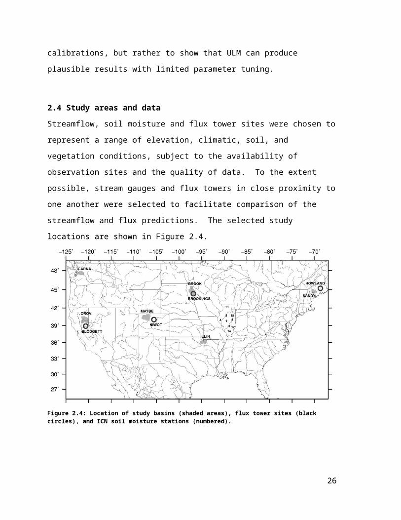
improvement in ULMM performance resulted from an increase in UZTWM, which
dampens the rapid storm runoff response, and increases low-flows slightly as well.
Figure 2.13: Daily streamflows and precipitation over the 1964 water year for the ILLIN (a) and BROOK (b) basins. Observed flow (solid black), ULMM (dashed black line), ULMA (dashed orange line), Noah (dashed pink line), and Sac (dashed green line) are included. These two basins provided the greatest challenge in modeling with relatively sporadic precipitation, and sharp streamflow peaks (BROOK: end of March snowmelt and soil thaw streamflow spike was poorly captured by the snow model and frozen soil physics).
BROOK is also characterized by low streamflow for most of the year, followed by large
surges in late spring and early summer, complicated by the effects of snowmelt and frozen
soil thawing which are not present (or negligible) at ILLIN. It has the lowest annual
precipitation of all study basins, and in part for this reason, all models struggle to capture
the peak flow response (Figure 2.13b) that is somewhat masked in the multi-year average,
as year-to-year differences in timing appear as a broad peak (see Figure 2.11). Most
notably, a substantial decrease in UZTWM is needed to increase model peak-response as
confirmed in both the parametric scatter plot in Figure 2.12, and the daily hydrograph
(Figure 2.13b).
30
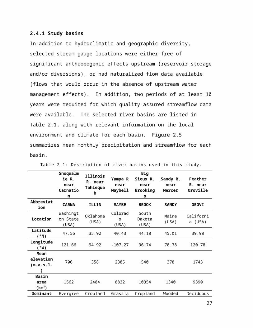
The impact of snowmelt is more visible in the hydrographs of the other four basins.
MAYBE has the lowest annual precipitation of these four and thus the soil response to
snowmelt is of great importance (since much of the winter precipitation is released in
spring as snowmelt). Noah and ULMA have flashy response to the large spring snowmelt,
while an increase in the upper-zone storage in ULMM, buffers the runoff rate to more
closely match observations. Sac, which uses a different snow model than Noah and ULM,
has similar streamflow timing to both ULMM and observations, however it has higher ET
rates (not shown), which ultimately result in an overall reduced hydrograph. Both the
OROVI and CARNA basins receive most of their precipitation between November and
March, of which a majority is stored as snow that ultimately runs off in the warm season.
The large surplus of water during melt season for these basins makes the larger lower zone
storages of increased consequence for accurately simulating baseflow, runoff, and ET rates
into the warm season. The wettest basin (CARNA) shows a marked improvement in
streamflow simulations when the lower zone hydraulic conductivity LZSK is reduced to
attenuate baseflow. Similarly, an increase in the lower zone storage LZFPM for the
OROVI basin provides for more realistic spring and early summer streamflow.
Precipitation over the SANDY basin is distributed nearly evenly throughout the year with a
slight peak in autumn. However, the storage and release of winter precipitation as
snowmelt in the spring is the dominant seasonal streamflow feature. It follows that a
reduction in LZSK attenuates the snowmelt response to yield a modest improvement in
streamflow in ULMM. Sac gets the peak timing correct, however with flows that are
generally too low, while the Noah peaks are too broad and low flows are overestimated.
One way to organize the importance of model parameters by basin is through classification
by an aridity index (AI); a metric first proposed by Budyko (1974):
AI = Rnet,ann/LPann (2.6)
Where Rnet-ann is the annual average net radiation, L is the latent heat of vaporization, and
Pann is the mean annual precipitation, such that LPann is the amount of energy needed to
evaporate the available precipitation, Pann. As AI exceeds 1, a basin becomes increasingly
arid (or water limited), whereas for AI less than 1 radiation becomes limiting (increasingly
moist), while the potential evaporation is theoretically reached at AI = 1. Comparing the
respective AI values for each basin and its most sensitive parameters in Table 2.5 highlights
31

the importance of upper zone parameters for more arid basins, and lower-zone parameters
for wetter basins. For water-limited basins, UZTWM plays a critical role in partitioning
infiltration and runoff, as well as controlling direct soil evaporation, while for all basins, an
increase of the allowable area that becomes impermeable during soil saturation (ADIMP)
was beneficial in capturing streamflow timing related to large moisture input events, such
as storms and snowmelt. Wetter basins benefited from an adjustment in the rate of
baseflow response from the larger lower-zone reservoir, where LZSK was lowered from its
a priori value and LZPK was increased.
Table 2.5: Aridity indices (AI) for each study basin and the key parameters for improved
streamflow, where a decreasing parameter is given in parentheses. Supplemental to the
parameters listed, the ADIMP parameter was increased to 0.225 for all basins.
Basin Annual AI
Seasonal AI Key ParametersDJF MAM JJA SONCARNA 0.3 -0.2 1.7 8.1 0.6 (LZSK), LZFSMSANDY 0.7 -0.9 3.3 5.5 1.4 (LZSK), LZPKILLIN 1.0 2.2 4.5 6.5 2.8 UZTWM, LZPK
OROVI 1.4 0.1 7.2 64.8 5.0 UZTWM, LZFPMMAYBE 1.6 -0.7 6.3 21.4 5.0 UZTWM, UZFWMBROOK 3.0 -2.0 15.6 13.9 7.8 (UZTWM), PCTIM
Table 2.6 lists the NSE for ULMA, ULMM, ULM3, Noah and Sac, computed for the six
study basins for both training and evaluation periods (i.e. 12 cases). Beginning with the
simulations using only a priori parameters (ULMA, Noah, Sac), ULMA scored highest 4
times, the median 6 times and the lowest 2 times. The latter cases were for the same basin
(BROOK – the most arid basin) for which none of the a priori simulations performed
distinctively better than climatology, so this was somewhat of an outlier. Considering the
entire set of simulations in Table 2.6, ULMM was the best model 9 times, ULM3 was best
twice, and Sac was best once. ULM3 was capable of realizing much of the performance
gains from ULMM for most basins, including 3 exceptions where it outperformed ULMM.
We attribute these exceptions to the random component in the ULMM parameter set
(inherent in the Monte Carlo procedure), whereas ULM3 used a priori values for less-
sensitive parameters that performed better in these cases. Sac outperformed all models
32
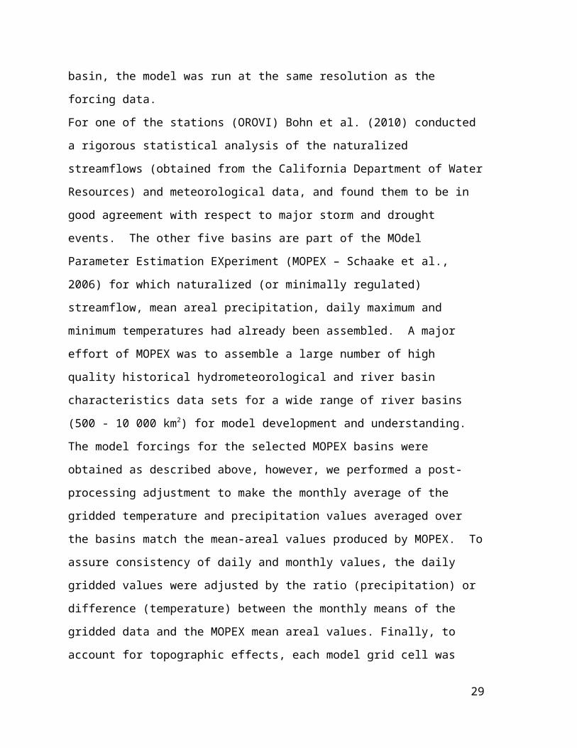
during the validation period in the snowmelt-dominated MAYBE basin, for which Sac’s
snow model was particularly well suited. Table 2.6: Summary statistics: Nash-Sutcliffe model efficiencies (in %) for training (1960 –
1969) and validation periods (1990 – 1999) for the Noah, Sac, and ULM models with a priori
parameters (ULMA), with a maximization of efficiency through a Monte Carlo experiment
(ULMM), and through adjusting only three parameters from their a priori values (ULM 3)
based on sensitivity and climate. Daily statistics are non-parenthesized and monthly
statistics in parentheses. Cases where ULM 3 scored higher than ULMM for the respective
period are bolded and any model scoring higher than ULM M was underlined.
Basin Training period Validation period
ULMA ULMM ULM3 Noah Sac ULMA ULMM ULM3 Noah SacSANDY 37.2
(81.2)51.2
(83.2)49.3
(81.7)32.3
(74.4)13.1
(22.1)27.7
(71.7)38.7
(70.8)40.5
(75.0)25.3
(52.9)20.0
(38.9)CARNA 0.5
(3.5)23.2
(50.1)21.0
(49.6)-5.8
(-6.5)-13.3(12.4)
1.8(54.5)
22.2(57.5)
20.8(54.3)
-5.5(48.1)
-4.8(36.9)
ILLIN 15.1 (67.0)
36.9(69.3)
31.9(52.8)
11.7 (23.1)
26.7 (54.8)
14.5(64.3)
48.2(76.8)
42.1(64.3)
22.0(69.2)
34.7(66.3)
MAYBE -12.8(-4.7)
64.3(74.3)
67.8(76.9)
-32.1(-22.6)
45.6(26.1)
-40.6(-6.2)
43.3(57.3)
42.0(62.3)
-98.0(-28.7)
47.1(38.4)
OROVI (46.9) (81.4) (59.3) (57.7) (38.7) (64.5) (80.0) (71.7) (46.7) (70.0)BROOK -11.0
(-22.1)18.2
(46.6)5.4
(2.8)2.2
(-10.1)-8.0
(-24.9)-29.1
(-47.1)5.7
(-5.9)-15.3
(-34.5)-27.1
(-43.9)-34.7
(-56.5)
In summary, ULMA performed comparably or slightly better than Noah and Sac for the
wetter basins, whereas it was generally on par or slightly poorer for the drier basins. With
several, or all parameters estimated (ULM3 and ULMM, respectively) significant
improvements were realized for all basins with the largest occurring for the drier basins.
The parameter adjustments of ULMM and ULM3 are underscored because unlike Noah and
Sac, ULM does not yet have an established set of default (or a priori) parameters. Such a
parameter set depends in large part on the dynamic equilibrium of model soil moisture,
which itself is dependent on the ET scheme, which come from Sac and Noah, respectively.
Therefore, the potential advantage of the model structure change was offset by the lack of
customized ULM-specific parameters for the ULMA comparisons.
An experiment was conducted in which the parameter adjustments from ULM3 and ULMM
were transferred to corresponding flux tower parameter sets, to attempt to improve model
results for both surface fluxes and soil moisture (where applicable). However, the resulting
33

simulations were not conclusively improved by this experiment, calling into question the
merit of the parameter transfer strategy. In addition, comparing the seasonal (JJA) and
annual AI values from basin to point, there were notable discrepancies
(BLODGETT/OROVI: AIJJA = 65.7/64.8, AIannual = 0.8/1.4; NIWOT/MAYBE: AIJJA =
9.1/21.4, AIannual = 1.5/1.6; HOWLAND/SANDY: AIJJA = 4.7/5.5, AIannual = 0.7/0.9;
BROOKINGS/BROOK: AIJJA = 8.7/13.9, AIannual = 1.5/3.0). The apparent lack of
transferability for Sac parameters is consistent with the findings of Gan and Burges (2006)
and also follows the findings for other models (e.g. Heuvelmans et al., 2004, Abdulla and
Lettenmaier, 1997). Alternate approaches likely will be required for effective parameter
transferability and regionalization of ULM.
2.6 Conclusions
The objective of this work was to assess the potential of ULM to improve upon the
weaknesses of its parent models, Noah and Sac, while taking advantage of their respective
strengths. Model performance was examined in ways relevant to the typical uses of these
models, including prediction of land-atmosphere moisture and energy fluxes and
streamflow. We established a default set of soil parameters for ULM which we expected
would perform differently from the Noah and Sac a priori values given an alternate
equilibrium state within the new model structure. Finally, we evaluated a simple approach
for transferring parameters estimated on the basis of basin streamflow prediction
performance for energy and moisture flux predictions.
Our key findings are:
(i) On the basis of observed flux data from 4 Ameriflux sites, the alternate soil
moisture states of ULM result in diurnal variations of surface fluxes that are on
par or modestly superior to Noah (Sac does not predict moisture or energy
fluxes other than evapotranspiration and runoff).
(ii) The nonlinearity of observed soil drying was better captured by ULM (as
compared with Noah), whereas soil moisture response during wetter periods
was more comparable between models. ULM had the smallest bias in a 10 site,
multi-year soil moisture comparison. ULM and Noah comparably matched the
observed seasonal cycle, with Sac’s seasonality notably too small.
34

(iii) ULMA generally out-performed the Noah and Sac models over wetter basins,
however performance was more variable for drier basins, for which parameter
adjustments were required to achieve competitive performance.
(iv) Much of the streamflow accuracy improvements achievable by calibration
(ULMM) can be realized by adjusting only 3 parameters (ULM3), while leaving
the remaining parameters at the a priori values of the parent models (Noah and
Sac).
(v) For drier basins, simulated streamflow was generally most sensitive to upper
soil zone parameters, while the opposite was generally true for wetter basins.
Overall, ULM performance was encouraging. Parameter adjustments were ultimately
needed to improve simulations comprehensively relative to the parent models. However,
this has to be tempered by the fact that a suitable set of default (a priori) parameters has not
yet been established for ULM, and the a priori parameters of its parent models may not be
fully representative of the alternative quasi-equilibrium state within the new model
structure. Work remains to find a reliable set of a priori parameters for ULM to further
improve simulations of both moisture fluxes (streamflow and soil moisture) and energy
fluxes without compromising one for the other. In its present form, ULM could be applied
for any simulations for which Noah and Sac are currently used, with essentially the same
capabilities for data assimilation and coupling as Noah. Additional testing will be required
to evaluate the impact of ULM on atmospheric feedbacks and lateral moisture
redistribution. Finally, further examination of parameter transfer strategies across gradients
of vegetation, topography, soils, and climate is in order that will make ULM more
applicable over large areas without the need for site-specific parameter estimation.
35

III. MULTI-CRITERIA PARAMETER ESTIMATION FOR THE UNIFIED LAND MODEL
This chapter has been published as a discussion paper in Hydrology and Earth System
Sciences (Livneh and Lettenmaier, 2012).
3.1 Introduction
The evolution of land surface models (LSMs) towards increasingly complex
representations of hydrologic and biophysical processes requires special attention to the
fidelity of the models in partitioning water and energy budget components. The traditional
validation of models using observations of a single prognostic variable can result in model
predictions that are inherently biased towards that variable (McCabe et al., 2005). The
evaluation of multiple model outputs (as opposed to single-output analysis, such as
streamflow) has received increasing attention (e.g. Gupta et al., 1999, Crow et al., 2003,
McCabe et al., 2005, Khu et al., 2008, Werth and Guntner, 2010, Milzow et al., 2011).
Among the variables other than streamflow that have been used for LSM evaluation are
evapotranspiration (Nandagiri, 2007), surface heat fluxes (Gupta et al., 1999; McCabe et
al., 2005), hydrochemical and isotope tracers (Son and Sivapalan, 2007; Lischeid, 2008;
Birkel et al., 2010), land surface temperature (Crow et al., 2003; McCabe et al., 2005),
snow water equivalent (MacLean et al., 2010), terrestrial water storage (Werth and Gunter,
2010; Milzow et al., 2010), and water table level (Khu et al., 2008). The more frequent use
of multivariate observations is attributable in part to their growing availability. Some
satellite-based observations now have periods of record exceeding a decade for single
sensors, and multiple decades for some multi-sensor merged records.
In the context of parameter estimation, multi-criteria analyses can aid in addressing the
issue of equifinality (Beven and Freer, 2001). The equifinality problem arises when
different parameter sets result in similar model performance. One approach to reducing
equifinality issues and quantifying uncertainties in model calibration is the Generalized
Likelihood Uncertainty Estimation (GLUE) framework of Beven and Binley (1992), which
can aid in selection of model calibration parameters through estimating the likelihood that
each parameter set is the true predictor of the system. A distribution of likelihoods among
36
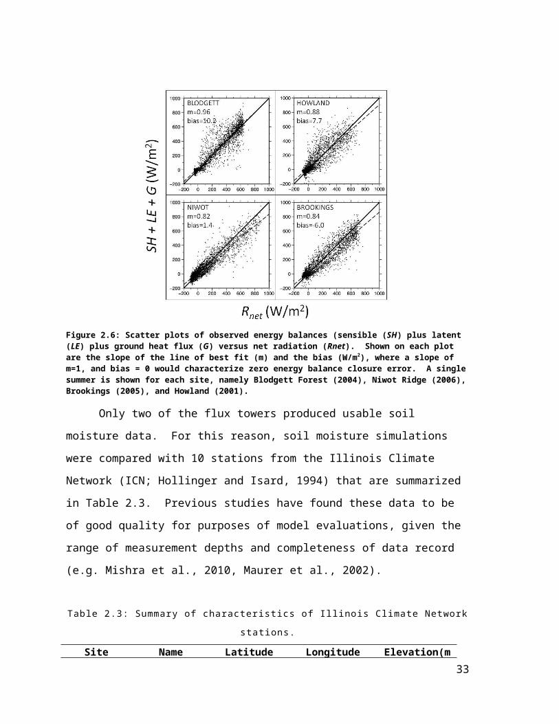
many parameter values is then generated and used to define uncertainties and select
parameters. Herein we consider an alternative calibration methodology (detailed in section
3.4) that selects parameters via ancillary objective functions. After identifying several top-
performing sets of model parameters, the addition of observational sources is used to
constrain parameter values – i.e. multivariate performance analyses. This reduces the
number of similar feasible parameter sets to allow selection of a single best parameter set
and hence produce robust parameter estimates. Robust model parameters are especially
important when models are used to predict outcomes for model forcings outside the range
observed in the model parameter estimation (calibration) period. Interannual variability of
streamflow regime is one such example, which provides a basis for the investigation of
potential future changes in river discharge that might result from climate or land-use
change (Kingston et al., 2011). Robust model parameters are also essential for examining
the importance of spatial and temporal scale on land surface response. Spatial scale can,
for instance, determine the nature of environmental impact assessments (João, 2002), and
the categorization of droughts (Shukla et al., 2011), but also determine how localized
hydrologic events propagate through a larger system (for instance, flash flooding from
tributary catchments as it affects the hydrologic response of a much larger region). The
accurate modeling of scale effects ultimately aids in decision making and issuing timely
warnings.
3.2 Modeling context
The Unified Land Model (ULM – Livneh et al., 2011) is the LSM used in this study. ULM
is essentially a merger of two widely used models: the Noah LSM (Ek et al., 2003; used in
most of NOAA’s coupled weather and climate models), and the Sacramento soil moisture
accounting model (Burnash et al., 1973; used for hydrologic prediction within the National
Weather Service). The parameter estimation experiments reported here can also be viewed
as a means to evaluate ULM rigorously in ways that extend the work of Livneh et al.
(2011). Additionally, given the ULM’s heritage and widespread use of Noah and Sac, the
implications of the results should be broadly relevant to the modeling community.
The objective of this work is to examine the benefits and potential tradeoffs of
incorporating multiple observations (multiple-criteria) into model calibration across a range
37

of hydroclimatic conditions and spatial scale. This will involve computing simultaneous
skill-scores between the model and each observed criteria. Using this information, the
nature of error accumulations and interannual variability in resulting model predictions can
also be examined.
We first apply a multivariate model calibration procedure over some of the major
river basins of the continental United States (CONUS), and follow with similar calibrations
for selected interior tributary catchments. Single and multi-criteria objective functions
were used to assess the added value of including information such as remotely sensed ET
and TWSC in the calibration procedure. Estimated parameters were then used to analyze
simulated streamflow variability, seasonality, and autocorrelation; examining both model
skill and error propagation across different spatial scales and hydroclimatic regions.
3.3 Data and Methods
In this section we describe the experimental design, including the study domain, the model,
and model forcing and evaluation data. We follow with a description of the model
calibration strategy and the trend and error analyses.
3.3.1 Basin selection, streamflow, and meteorological data
The study domain is comprised of river basins of different sizes within the CONUS,
selected to provide a broad cross section of hydroclimatic conditions and basin areas that
are representative of typical land surface modeling applications. The largest river basins
(hereafter major basins) are shown in Figure 3.1 and their characteristics are summarized in
Table 3.1. For several major basins, particularly in the western U.S., naturalized
streamflow data were obtained that have been adjusted for anthropogenic impacts,
including upstream (reservoir) regulation, water withdrawals and evaporation from
upstream reservoirs (see Table 3.1). In addition to the 10 major basins a set of 250 smaller
catchments (herein tributaries) were selected, most of which are tributaries to the major
basins (Figure 3.2). The tributaries are a subset of the MOPEX (Schaake et al., 2006) data
set, which have been screened to assure that they have an adequate density of precipitation
gauges and are minimally affected by upstream anthropogenic activities such as irrigation
diversion and reservoir operations. Hence streamflow observations for the tributaries were
38
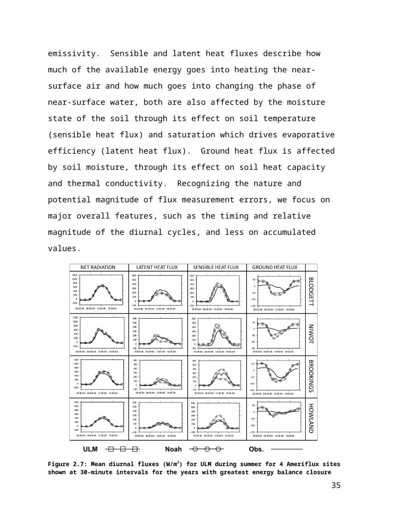
obtained directly from United States Geologic Survey (USGS) archives. All basins were
further screened here to have a minimum of 20 years of data with 100 % record
completeness within the period 1990-2009 to facilitate the use of remote sensing data sets
in multi-criteria parameter estimation.
Figure 3.1: Large-scale study domain, including precipitation gauges (black dots), as well as major hydrologic regions (shaded) that are defined through their drainage at stream gauges (blue circles). The un-shaded areas within these regions are either downstream of the stream gauge, or consist of many smaller river basins which drain directly into the Atlantic or Pacific Oceans or the Gulf of Mexico.
39

Table 3.1: Major hydrologic regions considered in this study including streamflow gauges
and drainage areas.
Hydrologic Region Abbreviation Applicable
criteriaStreamflow gauge location USGS ID Area (km2)
Arkansas-Red ARK Q*,ET,TWSC Arkansas R. near Little Rock, AR 07263450 409296
RED Q*,ET,TWSC Red R. at Index, AR 07337000 124397
California CALI Q*,ET,TWSC
Sacramento R. near Rio Vista, CA 11455420 69300
San Joaquin R. near Vernalis, CA 11303500 35058
Eastside streams and central valley floor ** 4655
Colorado COLO Q*,ET,TWSC Colorado R. above Imperial Dam, AZ 09429490 488213
Columbia CRB Q*,ET,TWSC
Columbia R. at Dalles, OR 14105700 613827
Columbia R. at Birchbank, BC 12323000 88101
Great Basin GBAS ET,TWSC N/A N/A 367602Lower Mississippi LOW ET,TWSC N/A N/A 221966
Upper Mississippi UP Q,ET,TWSC Upper Mississippi R.
at Grafton, IL 05587450 443665
Missouri MO Q*,ET,TWSC Missouri R. at Hermann, MO 06934500 1353269
Ohio OHIO Q,ET,TWSC Ohio R. at Metropolis, IL 03611500 525768
* indicates that naturalized flows were obtained
** unimpaired flow data for the Sacramento-San Joaquin River Delta were estimated by the California Department of Water Resources,
which receives a small contribution from eastside streams and flows from the central valley floor.
N/A – indicates that stream flow was not applicable; GB does not have an outlet at the basin boundary, LM represents the confluence of
multiple inflows and reliable flow data was not obtainable.
40

Figure 3.2: Small-scale study domain comprised of 250 tributary catchments using USGS stream gauges that were screened to be minimally affected by diversions, with at least 20 years of data in the past 3 decades to facilitate multicriteria comparisons.
The meteorological data used in this study were derived by Livneh et al. (2012) and are
available at a 1/16° resolution over the CONUS domain for the period 1915 – 2010.
Precipitation and daily minimum and maximum temperatures were obtained for the
National Oceanic and Atmospheric Administration (NOAA) Cooperative Observer (Co-op)
stations shown in Figure 3.1. Wind data were linearly interpolated from a larger (1.9°
latitude-longitude) NCEP–NCAR reanalysis grid (Kalnay et al. 1996) that was used to
produce daily wind climatology for years prior to 1948. For complete details of model
forcing data, see Livneh et al. (2012).
3.3.2 Auxiliary model evaluation data
In addition to streamflow observations, we made use of two independent estimates of ET,
which, like streamflow, are predicted by ULM. The first arises from an atmospheric water
balance over the major basins, whereas the second, derived from remote sensing, is
available on a spatially distributed basis, but for a relatively short (compared with most of
the streamflow records) period of roughly one decade.
41

3.3.2.1 Atmospheric water balance ET (ETAWB)
Computing an atmospheric water balance has been a long-standing means for studying
atmospheric exchanges of moisture over large areas. For a given atmospheric domain, with
vertical extent to the 100 millibar height
∇⋅1g ∫
100
ps
qV dp+ ∂∂ t ( 1
g ∫100
ps
q dp)=P−ET(3.1)
Where the first term is the convergence of liquid into, or out of the column, the second term
is the change in moisture (or precipitable water) from the column over time, q is the
specific humidity, V is the mean horizontal wind velocity, p is pressure at elevation, g is the
gravitational constant, and P is precipitation. Historically, the terms on the left-hand side of
equation 3.1 were obtained using a “picket fence” approach based on radiosonde
observations (e.g. Starr et al., 1965, Rasmussen, 1967, Rosen and Omolayo, 1981,
Ropelewski and Yarosh, 1998). Areal moisture fluxes could then be estimated by
integrating the divergence spatially over the domain, following Green’s Theorem. More
recent studies (Oki et al., 1995, Yeh et al., 1998, Syed et al., 2005, Yeh and Famiglietti,
2008) have used this approach, where the spatial fields come from atmospheric reanalyses,
which assimilate radiosonde data, as well as other satellite sources of information about the
vertical profile of moisture and temperature. Yeh et al. (1998) examined the lower limit of
spatial scale for applicability of the atmospheric water balance approach and found that
despite early estimates requiring areas >2 x 10⁶ km2 (Rasmussen, 1968), accurate
estimation of the climatology of regional evaporation is possible at scales as small as 105
km2. At spatial smaller scales smaller than about 105 km2, the accuracy of the estimates
degrades rapidly.
We use the North American Regional Reanalysis (NARR; Mesinger et al., 2006) as the
source of the two terms on the left-hand side of eq. 3.1, both of which are standard NARR
archived fields. The NARR output reflects the assimilation of radiosonde and satellite data
that are routinely used in numerical weather prediction, but performed with a “frozen”
version of the weather prediction model and data assimilation systems. The right-hand side
of equation 1 is based on the gridded precipitation fields derived from a network of
approximately 20,000 precipitation gauges across the continental U.S. by Livneh et al.
(2012). Figure 3 illustrates the atmospheric water balance as used in this study.
42
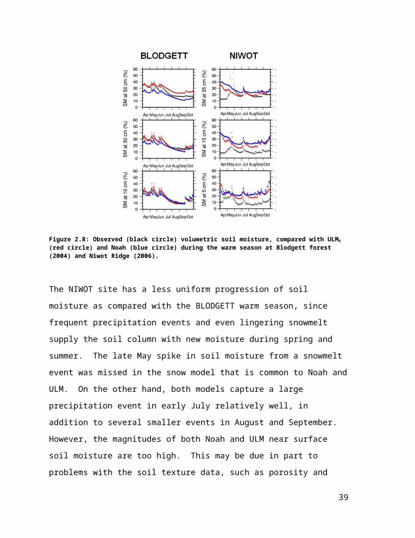
Figure 3.3: Example schematic of the Upper Mississippi river basin components needed to perform an atmospheric water balance to estimate ET (equation 3.1), including atmospheric moisture convergence, C, change in precipitable water, dPw/dt, and precipitation, P.
3.3.2.2 Satellite-based ET (ETSAT)
Satellite remote sensing provides a promising alternative to direct observations for
hydrologic prediction, although this is a source that has not been widely used to date – most
likely because satellite-based data record lengths are only now approaching a decade. We
used a MODIS-based ET data product produced by Tang et al. (2009). This product is
based on the VI-Ts method described by Nishida et al. (2003) which uses only satellite-
based (no surface data) products. Specifically, downward solar radiation is from the SRB
data set of Pinker and Laszlo (1992), based on Geostationary Operation Environmental
Satellites (GOES) and vegetation index (VI) and surface temperature (Ts) data are from
MODIS. Two key assumptions of the algorithm are a) that the evaporative fraction is
constant over the diurnal cycle, and is well estimated by values from the daytime satellite
overpass (of EOS/Terra in this case), and b) there is a substantial variation in VI-Ts pairs
over a local region, such that an upper envelope of VI and Ts can be defined. The reader is
referred to Tang et al. (2009) and Nishida et al. (2003) for details of the algorithm. The
43

algorithm was applied at 0.05° spatial resolution, where each pixel represents the average
of an area with 0.25° radius, to address assumption (b) above.
Comparing this approach with ground observations, Tang et al. (2009) computed
instantaneous and daily mean ET differences of less than 10% and 15% on average,
respectively. VI-Ts derived ET agreed favorably with estimates from a much higher
resolution Landsat-based method over irrigated areas of the Klamath River Basin in the
western U.S. Nishida et al. (2003) found correlations of R2>0.85 at 13 flux tower sites over
CONUS. Kalma et al. (2008) surveyed a number of satellite-based ET methods (including
the Nishida et al. VI-Ts method) and noted they can provide good estimates of the
catchment’s average evaporation on a daily basis subject to cloud cover. However, they
found that an important uncertainty in the ET estimates resulted from land surface
temperature errors from the satellite estimates that could be as great as 3-5K due to
atmospheric effects. Ferguson et al. (2010) analyzed a similar satellite-based ET product
and argued that a significant issue with satellite-based ET products is that they are not
constrained by soil/surface water availability. They found that in some cases the high ET-
demand during the warm season results in satellite-based ET estimates that are
unrealistically large.
3.3.2.3 Terrestrial Water Storage Change (TWSC)
The terrestrial water balance can be written as the difference between precipitation,
P, and streamflow, Q, and ET:
TWSC = P – Q – ET (3.2)
Storage plays a key role in the Earth’s climate system and the supply of freshwater for
human use, via interaction with groundwater, soil moisture, plant water, snow, and land-
ice. The Gravity Recovery and Climate Experiment (GRACE) provides a basis for
estimating monthly variations of TWSC over areas order of 105 km2 based on the effect of
TWSC on changes in the Earth’s gravitational field measured by a pair of satellites.
Temporal gravity variations at these spatial and temporal scales are mainly caused by mass
redistribution in the atmosphere and oceans, tides, postglacial rebound, and terrestrial water
cycling (Klees et al., 2008). Monthly gravity field solutions are computed at the University
of Texas at Austin Center for Space Research (CSR), the GeoForschungsZentrum
Postsdam (GFZ) and the Jet Propulsion Laboratory (JPL), which use different processing
44

strategies and hence yield slightly different results. Similar to Werth and Gutner (2010), we
used an average of GRACE gravity fields from these three processing centers (differences
among the data sets can be considered a measure of data uncertainty). Lo et al. (2010),
Werth and Guntner (2010), and Milzow et al. (2011) have shown the potential for using
GRACE-derived TWSC data in the calibration of LSMs However, the GRACE record
length is relatively short (from 2002), and the coarse spatial resolution complicates
comparisons with model predictions for other than very large river basins.
3.3.3 Land surface model
Livneh et al. (2011) provide a complete description of ULM as used in this study.
In general, the land surface components are from the Noah LSM – e.g., vegetation, ET
computation, snow model, and algorithms for computing frozen soil, surface heat and
radiative fluxes – whereas the subsurface elements (soil moisture and runoff generation
algorithms, as well as infiltration) are from Sac. The snow model is described by Livneh et
al. (2010). It essentially is the standard Noah snow model augmented to include time-
varying albedo, partial snow cover, and retention of liquid water within the snowpack.
Livneh et al. (2011) tested ULM at a small number of catchments and evaluated
performance with respect to observed river discharge, flux towers measurements of surface
heat fluxes, and soil moisture. Table 3.2 summarizes plausible physical ranges of the
model soil parameters that constrained the parameter estimation here.
45
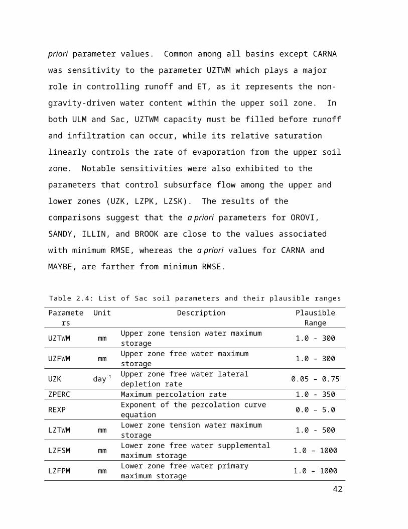
Table 3.2: List of ULM soil parameters from Sac and their plausible ranges.
Parameters Unit Description Plausible RangeUZTWM mm Upper zone tension water maximum storage 1.0 - 300UZFWM mm Upper zone free water maximum storage 1.0 - 300UZK day-1 Upper zone free water lateral depletion rate 0.05 – 0.75ZPERC - Maximum percolation rate 1.0 - 350REXP - Exponent of the percolation curve equation 0.0 – 5.0LZTWM mm Lower zone tension water maximum storage 1.0 - 500
LZFSM mm Lower zone free water supplemental maximum storage 1.0 – 1000
LZFPM mm Lower zone free water primary maximum storage 1.0 – 1000
LZSK day-1 Depletion rate of the lower zone supplemental free water storage 0.01 – 0.8
LZPK day-1 Depletion rate of the lower zone primary free water storage 0.0001 – 0.025
PFREE - Percolation fraction going directly from upper zone to lower zone free water storages 0.0 – 0.8
PCTIM - Impervious fraction of the ground surface 0.0 – 0.1
ADIMP - Maximum fraction of additional impervious area caused by saturation 0.0 – 0.45
3.3.4 Calibration procedure and error analysis
By far the most common method for hydrologic model calibration is through minimization
of differences between modeled and observed streamflow. The goal here was to extend
this approach to include auxiliary observational data sources to evaluate and constrain
model performance within a multi-criteria framework. The Nash-Sutcliffe efficiency (NSE
– Nash and Sutcliffe, 1970) was chosen to quantify model performance. NSE is given as:
NSE=1−∑t=1
n
( x s ,t−xo ,t )2
∑t=1
n
( xo ,t−μo )2=1−MSE
σ o2 (3.3)
Where xo,t and xs,t are the observed and simulated values at each time-step, µo is the
observed mean and n is the total number of time-steps. NSE is useful in comparing inter-
basin performance, since it normalizes the mean squared error, MSE, by the observed
variance, σo2, of each basin, where an NSE value of 1 corresponds to a perfect model, while
any value less than 0 describes a model that performs worse than simply using µo as the
predictor. As described by Gupta et al., 2009, the NSE may be decomposed to represent
the correlation between model and observed calibration variables (e.g. streamflow),
46

difference of means, and difference of standard deviations between simulations and
observations. They argue that calibrating a model within a multi-objective perspective
towards these three components is preferred as it enables better hydrological interpretation
of the solutions.
We performed optimizations using the MOCOM-UA algorithm, first developed by Yapo et
al. (1998), as a means of maximizing NSE (minimizing model errors) and its components
within a multiple objective framework. MOCOM-UA is a Pareto-based approach that
yields an optimal front (or surface) in an N-dimensional space, where N is the number of
objective-functions. The resulting set of parameters from the Pareto solution defines
parameter uncertainty attributable to model structural errors (Vrugt et al., 2003), in which
optimizing one objective function, has the trade-off of reducing the performance of
another. In our implementation, the calibrations were first performed on the individual
criteria specifically Q, both ET products, and TWSC to obtain an optimal set of model
parameters by minimizing errors in the components of NSE. Next, the same procedure was
applied to combinations of these criteria, maximizing their individual NSE, to determine
the trade-offs between single and multi-criteria analyses. The relative impact of
calibrations on model performance with respect to different criteria was further quantified
through changes in the relative root mean squared error (rRMSE). This metric provides an
additional means for inter-basin comparison, because it is a normalized measure that is
(nearly) independent of basin or process scale.
For each basin, the performance of the calibrated model was assessed relative to model
performance with default parameters (described in greater detail by Livneh et al., 2011)
herein CONTROL. The default parameters are comprised of the Noah LSM land surface
characteristics from the National Land Data Assimilation System (NLDAS – Mitchell et
al., 2004) and Sac parameters based solely on soil texture (Koren et al., 2003). For the
major basins (section 3.2.1) we also evaluated the utility of incorporating ET (atmospheric
balance and remote sensing) and TWSC as described in sections 3.2.2.1-3.2.2.3. The
tributary catchments are an order of magnitude too small for use of either atmospheric
balance ET or GRACE-based TWSC, and hence calibrations for these catchments used Q
and ETSAT.
47

To further evaluate model performance, an analysis of the variability of hydrologic
response in both major basin and tributary streamflows was conducted, followed by an
examination of model errors at two selected basins. Three components of model response
were examined: the lag-1 autocorrelation (persistence), coefficient of variation
(variability), and runoff efficiency (precipitation partitioning).The model’s ability to
reproduce these observed components, quantifies its representation of seasonality, and its
applicability for flood forecasting under different climate scenarios.
In the final part of the analysis, a subset of the domain was selected to further detail model
errors. Examining hydrographs of selected major basins and their tributaries provides an
additional means to understand the nature of differences between simulated and observed
flows and if it is possible to predict how these errors may propagate within a given region.
Lastly, overall uncertainties in the model and observational data are discussed including the
manner in which they may affect this study’s conclusions.
3.4 Results and Discussion
We present single-criterion calibration results from the major basins first, followed
by the tributary single-criteria calibrations. We then present and discuss multi-criteria
calibration results for both major and tributary basins. Finally, two regions are selected for
a general examination of model errors.
3.4.1 Single criterion calibrations
We first calibrated ULM using a single criterion approach based on streamflow simulation
errors with the objective functions of the NSE components. Figure 3.4 shows the results of
model calibration to streamflow over major basins. Nearly all basins show calibrated
streamflows that follow closely with observations. Notable improvements in modeled
streamflow were realized over COLO, despite the quantitatively poorer performance
compared with other basins (performance statistics presented in the next section).
Streamflow simulation errors were noted by other investigators over COLO using the Noah
LSM (Xia et al., 2011, Vano et al., 2011) which is relevant to the ULM simulations given
its heritage from Noah. Errors were attributed to the significant changes that were made to
the Noah canopy parameterizations in its latest official NCEP version (v2.8 – noted by Wei
48

et al., 2012) such as stomatal resistance, seasonal leaf-area index (LAI), and root
distribution, all of which affect ET and runoff generation. These changes generally
improved performance, however the Colorado basin was an exception that was
compensated for here by ULM calibrations that allow for greater soil moisture capacity to
store and release large snow melt volumes. For other regions, such as CALI and OHIO,
control simulations were fairly skillful at capturing dynamics of seasonal low flows, such
that only small improvements were obtained from calibrations. For the remaining regions
runoff ratios were generally too high in the CONTROL simulation, requiring in most cases
slight reduction in hydraulic conductivity and increases in moisture holding capacity and
permeability parameters.
Figure 3.4: Mean monthly hydrographs in m3/s for the major basins for a 20 year period, the beginning of which varies by basin, depending on data availability.
49
To quantify the relative uncertainty of the two remote sensing ET products, Figure 3.5
compares them with the long term difference (P-Q) between observed precipitation, P, and
streamflow, Q. The underlying assumption in this comparison is that over a sufficiently
long time, the net change in soil moisture storage will become small and the ratio of ET to
the difference P-Q, will approach unity. It should be noted that the ETAWB and ETSAT
products are for different periods (1979-2010, and 2001-2010, respectively) and are plotted
together to facilitate an initial approximation. In nearly all cases (except RED) ETAWB is
larger than P-Q, corresponding to either a negative change in TWS, or measurement
uncertainty. ETSAT is available for both major and tributary basins, where CALI is the only
case with ETSAT > P-Q for a major basin as well as the mean of all of its tributaries. This
consistent bias, if not an artifact of estimation error, implies a long term (2001-2010) loss
of terrestrial water storage. Tang et al. (2009) tested this algorithm over northern California
and found a slight high bias in ET compared with ground-based Bowen ratio stations,
suggesting that the positive bias seen here could be due in part to the algorithm itself. ETSAT
for all other major basins was slightly less than unity, where the mean of the respective
tributaries were also less than unity The general form of the scatter in Figure 3.5 shows
increasing ETSAT negative bias with increasing P-Q, characterized by a pseudo-linear slope
of slightly less than one. The mean relative biases on the order of 10 – 20% are due either
to the ETSAT algorithm, TWS, observational uncertainty in P and Q, or some combination of
these.
50

Figure 3.5: Estimates of mean monthly evapotranspiration by an atmospheric water balance (ETAWB – section 2.2.1) in squares, and through satellite data (ETSAT – section 2.2.2) in circles compared with the residual of precipitation, P, minus streamflow, Q, for the major basins and smaller tributaries (smaller circles). Shaded areas denote the domain within which ET was estimated, such that un-shaded circles represent ET from tributaries outside the major basins.
The requirement of variation of VI-Ts in the ETSAT derivation method is examined in
Figure 3.6 through a comparison of the long-term residual term, P-Q-ETSAT, and the VI and
Ts diversity of each basin. Basin-wide ETSAT monthly averages are shown, which were
computed from 0.05° pixels (described in section 3.3.2.1). With the exception of CALI, the
large basins have a consistently small residual term and a larger VI-Ts diversity as
compared with their tributaries. The bias in Figure 3.6 appears to be irrespective of the VI-
Ts diversity, or at minimum does not imply decreasing water balance residual with
increasing VI-Ts diversity. Mean NDVI ranges by basin vary from approximately 11-115,
while skin temperature ranges vary from 46-72K throughout the simulation period. For
example, the tributaries of MO possess among the smallest VI-Ts product range, while
51

their water balance residuals are near zero, while basins from CALI have larger VI-Ts
diversity products with comparatively larger water balance residual. The implications of
Figure 3.6 for this analysis are that these basins possess adequate VI-Ts diversity for the
ETSAT algorithm. Alternatively stated, the relative VI-Ts diversity alone cannot be used as a
means to qualify or disqualify the ETSAT data used here for model calibration.
Figure 3.6: Comparisons of the residual of evapotranspiration from satellite data (ETSAT –section 3.2.2.2) with precipitation, P, minus streamflow, Q, for the major river basins (larger circles) and smaller tributaries (smaller circles) 2001 – 2010, as a function of VI-Ts diversity, expressed as a product of the ranges of NDVI and skin temperature for each basin. Departures from the dashed line denote either an uncertainty in ET estimates, or significant long-term TWS, or other observational errors.
The two remote sensing ET sources show notable seasonal differences in Figure 3.7. For
all basins, the ETAWB peaks earlier in the year on average relative to ETSAT, with greater
peak magnitude in all cases except CALI. The calibrations were most effective in
improving the seasonality and timing of peak ET, whereas calibration improved total ET
(monthly) magnitude only for cases where the CONTROL ET was already larger than the
52
respective remote sensing ET product . For cases where either ETSAT or ETAWB were
appreciably larger than simulated control ET (most frequently for ETAWB), the calibrated
ET remained less than the respective ET product. This difference in ET magnitude was
greatest for the western-most basins, which generally exhibit warm-dry summers with large
ET demand. This discrepancy comes about in part because of the constraint imposed by
ULM’s water balance, something that the remote sensing products don’t reflect, and often
plays a role when ET demand is high. Over the cold-season (DJF), calibrated-ULM
frequently matched ETSAT, whereas the larger cold-season ETAWB exceeded the calibrated
model estimates at all but ARK and LOW, which have comparatively mild cold-seasons.
Notwithstanding the western-most basins, the differences between the calibrated model and
the respective ET (calibration objective-function) in Figure 3.7 are notably less than the
difference between the two remote sensing data sets, which can be considered a measure of
observational uncertainty.
53

Figure 3.7: Mean monthly ET (mm) for the major river basins for the period 2001 – 2010 that include two sets of calibrations, satellite-based (SAT) or atmospheric water balance-based (AWB) observational products as well as the control simulation.
The seasonal cycle of modeled TWSC has similar amplitude to the GRACE product for
most of the basins, as shown in Figure 3.8. In nearly all cases, calibration brings the mean
simulated TWSC within the envelope of observational uncertainty for mean TWSC
(denoted by the dark-gray shading). In relative terms, the CALI region has the largest
seasonal cycle for both the observed and simulated signals, while regions such as ARK,
GBAS, and MO, have much smaller amplitudes that are well replicated by ULM. Modest
TWSC discrepancies can be expected since we are comparing the model – which is
constrained by a relatively shallow (~ 2m) water balance – to the unconstrained estimate of
TWSC made by GRACE, which may include contributions from deep groundwater
movement and has a coarser native spatial resolution.
54

Figure 3.8: Mean monthly TWSC (mm) for the major river basins for the period 2002-2010 including the control and calibrated model simulations; the range of variability for each case is shown accordingly.
The single-criteria calibrations for the tributaries were organized by classifying each
catchment by its aridity index, AI; a metric first proposed by Budyko (1974):
AI = Rnet,ann/LPann (3.4)
In which Rnet-ann is the annual average net radiation, L is the latent heat of vaporization, and
Pann is the mean annual precipitation, such that LPann is the amount of energy needed to
evaporate the available precipitation, Pann. AI values exceeding 1 denote increasingly arid
(or water limited) conditions, whereas values less than unity denote moist (or radiation
limited) conditions. Figure 9 shows the resulting daily calibrated NSE values for the
tributaries. Daily NSE values are expected to be smaller than for monthly flows, due to the
increased variability in observed flows at the finer temporal scale, which is indeed the case
in Figure 3.9. A large number of the total tributaries have AI between 0.6 and 1.2. With the
55

exception of two tributaries of RED, the model performance appears to decrease with
increasing AI, beginning at AI ≈ 0.6. Figure 3.10 shows a similar plot but for ET
calibrations. Given the seasonality of ET and its strong dependence on atmospheric forcing
– i.e. downwelling radiation – many of the tributaries have NSE values above 0.6, with
higher NSE values than for the corresponding Q calibrations. However, for a small number
of cases (6), ET calibration could not raise model NSE above zero – e.g. less skill than
climatology. These disagreements result from cases in the southern part of the domain
where ETSAT values are not constrained by water availability (arid basins) and peak ETSAT
values are in some cases greater than twice the peak modeled values. Notwithstanding
specific NSE values for the aforementioned single-criteria calibrations, the degree of
improvement resulting from calibration relative to the CONTROL case is presented in
greater detail in the following section.
Figure 3.9: NSE values for ULM calibrations to streamflow at a daily time step as a function of AI for the period 1991-2010. Shading of individual points denotes the major region for each tributary.
56
Figure 3.10: NSE values for ULM calibrations towards ETSAT at a daily time step as a function of AI for the period 2001-2010. Shading of individual points denotes the major region for each tributary.
3.4.2 Multi-criteria calibrations
A central objective of this study was to examine the extent to which calibration towards
multiple criteria could improve model simulations relative to each of the criteria. A visual
representation of the multi-criteria calibration for the major basins is shown in Figure 3.11,
while the entire set of results are tabulated in Table 3.3 and Table 3.4. The three axes in
Figure 11a represent objective functions (NSE) geared towards minimizing modeled errors
in, Q, ET, and TWSC, respectively. Within each calibration set, a single optimal solution
was selected that represents a tradeoff between optimizing its respective objective
functions, giving equal weight to each. For example, the calibration labeled Q,ETAWB
produced a set of simulations that minimized the objective functions for each of these
quantities (Q and ETAWB), creating an envelope of similarly scoring simulations (a Pareto
front). In order to select the optimal calibration from among these, the simulations which
57

best minimized errors in the auxiliary criterion – in this case TWSC – was chosen. From
Figure 3.11a it is clear that single-criterion calibrations often lead to poor performance in
the other criteria. The exceptions to this pattern are the single criterion Q-calibrations,
which have the largest number of simulations closest to the ideal point (1.0,1.0,1.0).
Double and triple-criteria calibrations that include Q, were generally the next closest to
ideal, with those containing TWSC generally more successful. Conversely, calibrations that
did not include Q more frequently performed poorly in one or more criteria, as this lack the
implicit overall water balance associated with high fidelity Q simulations – i.e. the timing
and partitioning of surface runoff, which encompasses water availabilities for both ET and
TWSC. It is assumed here that the observational uncertainty associated with the ETSAT,
ETAWB, and TWSC objective functions are larger than for Q observations.
Figure 3.11: ULM calibrations over major basins towards combinations of Q,ETSAT, ETAWB, and TWSC at a monthly time step for the period 1991-2010, including (a) NSE values for each criteria (cutoff at -1 for clarity), and (b) differences in rRMSE for each criteria resulting from the respective calibrations. The entire set of results for these plots is included in Table 3.3 and Table 3.4.
58

Table 3.3: Summary of skill scores and improvements from the single-criterion calibrations;
numeric values show improvement, while dash cells indicate no improvement in model skill
for the respective variable. Underlined values denote the specific ET observation to which
calibration was performed.
Calibration quantity
NSE skill rRMSE improvementBasin Q ETAWB ETSAT TWSC Q ETAWB ETSAT TWSC
Q
ARK 0.85 0.88 0.89 0.17 1.68 0.06 0.18 2.88RED 0.78 0.81 0.70 0.37 2.65 0.15 0.19 2.03CALI 0.94 0.75 0.10 0.53 0.48 0.20 0.02 4.19COLO 0.46 0.57 0.50 0.32 5.78 0.14 0.11 6.01CRB 0.78 0.50 0.63 0.69 0.77 0.06 0.14 7.30MO 0.87 0.77 0.74 0.61 1.76 - - 11.49OHIO 0.86 0.68 0.76 0.43 0.21 - 0.02 0.80UP 0.72 0.54 0.56 0.20 0.46 - - 2.60
ETAWB
ARK - 0.93 0.76 0.03 - 0.11 0.08 -RED - 0.89 0.62 0.39 - 0.21 0.15 2.66CALI 0.22 0.84 0.36 0.41 - 0.27 0.11 2.17COLO - 0.61 0.56 0.05 3.65 0.15 0.13 2.63GBAS - 0.62 0.43 0.57 - 0.21 0.23 3.23CRB - 0.63 0.54 0.67 - 0.13 0.08 6.96LOW - 0.92 0.76 0.42 0.00 0.05 0.04 6.17MO - 0.93 0.78 0.47 0.36 0.02 - 6.92OHIO 0.15 0.92 0.74 0.37 - 0.05 0.00 -UP - 0.93 0.82 0.04 - 0.10 - -
ETSAT
ARK - 0.81 0.96 - - - 0.27 -RED - 0.77 0.90 0.32 - 0.12 0.32 0.62CALI 0.45 0.45 0.65 0.31 - 0.03 0.24 0.75COLO - 0.53 0.69 0.02 3.16 0.12 0.20 2.26GBAS - 0.59 0.53 0.60 - 0.20 0.27 3.57CRB - 0.45 0.65 0.27 0.05 0.04 0.15 1.43LOW - 0.73 0.97 0.20 0.15 - 0.26 1.62MO - 0.78 0.96 0.20 - - 0.22 -OHIO - 0.71 0.96 0.32 - - 0.25 -UP - 0.84 0.96 0.06 - - 0.21 -
TWSC
ARK - 0.80 0.87 0.37 - - 0.16 11.49RED - 0.55 0.24 0.57 - 0.02 0.00 8.38CALI 0.15 0.71 0.07 0.47 - 0.17 0.00 3.22COLO - 0.11 0.26 0.19 2.53 0.00 0.01 4.25GBAS - 0.59 0.48 0.59 - 0.20 0.25 3.52CRB - 0.53 0.54 0.68 - 0.07 0.07 7.17LOW - 0.77 0.63 0.58 - - - 9.97MO - 0.91 0.82 0.52 0.52 - 0.02 8.49OHIO 0.39 0.69 0.54 0.55 - - - 2.70UP - 0.75 0.76 0.42 0.13 - - 7.75
59

Table 3.4: Same as Table 3.3, except for multi-criteria calibrations.
Calibration quantity
NSE skill rRMSE improvementBasin Q ETAWB ETSAT TWSC Q ETAWB ETSAT TWSC
QETAWB
ARK 0.59 0.89 0.74 - 1.43 0.07 0.06 -RED 0.09 0.81 0.57 - 2.14 0.15 0.13 -CALI 0.68 0.64 0.27 0.40 0.13 0.13 0.08 2.04COLO - 0.55 0.55 0.09 4.11 0.13 0.13 3.06CRB - 0.16 0.26 0.41 0.21 - - 3.10MO - 0.87 0.77 0.29 1.24 - - 2.06OHIO 0.74 0.89 0.76 0.47 0.12 0.01 0.02 1.40UP 0.71 0.86 0.81 0.31 0.45 0.02 - 5.18
QETSAT
ARK 0.50 0.87 0.75 - 1.36 0.04 0.07 -RED - 0.74 0.54 - 2.02 0.10 0.11 -CALI 0.71 0.45 0.62 0.35 0.15 0.03 0.22 1.29COLO - 0.55 0.69 0.02 3.95 0.13 0.20 2.26CRB - 0.19 0.58 0.42 0.35 - 0.10 3.31MO - 0.86 0.72 0.22 1.25 - - 0.25OHIO 0.69 0.78 0.77 0.38 0.09 - 0.03 0.04UP 0.60 0.88 0.82 0.23 0.39 0.04 - 3.35
Qtwsc
ARK 0.46 0.87 0.68 0.18 1.35 0.04 0.03 0.68RED - 0.82 0.66 0.45 - 0.15 0.17 4.34CALI 0.71 - - 0.38 0.17 - - 1.81COLO - 0.53 0.60 0.05 4.21 0.13 0.15 2.65CRB 0.09 - 0.01 0.40 0.39 - - 3.04MO 0.06 0.87 0.75 0.27 1.30 - - 1.67OHIO 0.73 0.85 0.71 0.50 0.11 - - 1.82UP 0.55 0.63 0.65 0.32 0.37 - - 5.45
ETAWBTWSC
ARK - 0.88 0.86 0.35 - 0.06 0.15 10.13RED - 0.59 0.32 0.49 - 0.03 0.03 5.46CALI 0.15 0.76 0.11 0.43 - 0.21 0.02 2.47COLO - 0.64 0.63 0.14 3.94 0.17 0.17 3.68GBAS - 0.59 0.47 0.59 - 0.20 0.25 3.50CRB - 0.56 0.56 0.69 - 0.09 0.09 7.30LOW - 0.85 0.71 0.58 - - 0.00 9.92MO - 0.93 0.79 0.50 0.66 0.02 - 7.95OHIO 0.42 0.90 0.71 0.54 - 0.02 - 2.46UP - 0.88 0.80 0.37 0.13 0.04 - 6.66
ETSATTWSC
ARK - 0.89 0.89 0.32 - 0.05 0.18 8.08RED - 0.79 0.79 0.43 - 0.13 0.24 3.62CALI 0.52 0.70 0.70 0.38 0.00 0.20 0.27 1.81COLO - 0.71 0.71 0.10 3.31 0.12 0.21 3.23GBAS - 0.50 0.50 0.59 - 0.12 0.26 3.53CRB - 0.40 0.50 0.30 0.94 0.16 0.18 2.54LOW - 0.77 0.77 0.52 - - 0.05 8.40MO - 0.82 0.82 0.49 0.55 - 0.02 7.65OHIO 0.39 0.79 0.79 0.48 - - 0.04 1.46UP 0.42 0.81 0.81 0.38 0.32 - - 6.88
QETAWBTWSC
ARK 0.43 0.89 0.71 - 1.33 0.06 0.04 -RED - 0.80 0.47 - 2.04 0.14 0.09 -CALI 0.63 0.64 0.41 0.37 0.09 0.13 0.13 1.59COLO - 0.53 0.60 0.05 4.21 0.13 0.15 2.65CRB - 0.11 0.39 0.63 0.31 - - 6.36MO - 0.92 0.80 0.40 0.54 0.11 0.14 1.83OHIO 0.73 0.88 0.72 0.51 0.11 0.01 - 1.95UP 0.53 0.77 0.77 0.27 0.36 - - 4.13
QETSATTWSC
ARK 0.49 0.73 0.73 - 1.37 - 0.06 -RED - 0.46 0.46 - 1.97 - 0.08 -CALI 0.63 0.41 0.41 0.37 0.09 0.06 0.13 1.59COLO - 0.60 0.60 0.05 4.21 0.06 0.15 2.65CRB 0.09 0.01 0.01 0.40 0.39 - - 3.04MO - 0.80 0.80 0.30 1.04 0.11 0.09 2.83OHIO 0.74 0.74 0.74 0.45 0.12 - 0.01 1.12UP 0.63 0.79 0.79 0.34 0.41 - - 5.76
The extent to which each criterion was improved through calibration is illustrated in Figure
3.11b, quantified by the rRMSE difference with each basins CONTROL simulation.
Examining this figure along with the accompanying tables (Table 3.3, 3.4), it is clear that
60
calibrations to certain criteria have the potential to either improve or worsen model
performance towards other criteria. Very generally, the results form a central cluster with
three branches. The central cluster of simulations is comprised mostly of multi-criteria
calibrations that exhibit modest improvements in each criterion. This modest improvement
in each criterion is consistent with the degree of improvement noted by Gupta et al. (1999)
for their multicriteria calibrations towards surface heat fluxes. The lower branch is made up
mostly of single-criteria ET calibrations (ETSAT,ETAWB) that exclusively improve ET
performance, for cases where the objective function conflicts with the other criteria, and
hence worsens the performance in other criteria. The upper-left branch is made up of
calibrations for which there is good agreement between the ET and TWSC data, and hence
large improvements in these objective functions through calibration. The upper-right
branch follows similarly except with agreements between TWSC and Q data.
This analysis suggests that at the regional scale (larger than ≈ 105 km2), calibrations
towards Q are generally more robust than those towards TWSC and ET in a multi-criteria
context. Overall, the remote-sensing auxiliary criteria (ETAWB, ETSAT, TWSC) generally
provide useful information regarding the seasonality of the terrestrial water balance.
However, these criteria alone or in combination do not appear sufficient to appreciably
improve model simulations of Q, as may be the desire in an ungauged basin.
Figure 3.12 shows multi-criteria results for the tributaries and follows the same format as
Figure 3.11 with considerably more data points for the Q and ETSAT criteria. In contrast to
the major basin results in Figure 3.11a, Figure 3.12a shows that the multi-criteria
calibration (Q,ETSAT) for the tributaries performs competitively with both single-criterion
calibrations in terms of NSE for a large number of tributaries. For all calibration criteria,
there are basins that perform poorer than climatology – i.e. NSE < 0 – however these are
mostly for single-criterion calibrations relative to the other criterion. For example, it
follows intuitively that the ETSAT calibration has instances of poorer NSE with respect to Q,
than does the Q,ETSAT calibration. Figure 3.12b shows quantitatively greater improvements
in Q performance than ET (note that the horizontal axes are not the same in this plot). This
reflects the greater flexibility in model structure and (soil) parameter combinations
considered here to influence Q outputs versus ET with relation to a given set of
atmospheric forcings. For both Q and ETSAT, rRMSE improvements in single-criterion
61
calibrations were frequently made at the expense of rRMSE of the other criterion. An
interesting finding is that the top Q simulations from approximately one third of all
tributaries (81) resulted from multi-criteria Q,ETSAT calibrations. This is in direct contrast
to the major basin calibrations, in which the top performing Q simulations resulted
exclusively from single-criterion Q calibrations, For only six tributaries (~2 % of all
tributaries), ETSAT calibrations improved Q to a comparable degree to Q calibrations.
Therefore, consistent with the major basin analysis, the use of only auxiliary remote-
sensing criteria (in this case, only ETSAT) was not sufficient to appreciably and reliably
improve Q performance. The unique conclusion here is that the inclusion of an auxiliary
remote sensing criterion (Q,ETSAT) for the tributary basins (<104 km2) can improve
calibration results beyond that of the single-criterion calibration.
Figure 3.12: ULM calibrations over tributary basins towards combinations of Q, and ETSAT at a daily time step for the period 1991-2010, including (a) NSE values for each criteria and (b) differences in rRMSE for each criteria resulting from the respective calibrations.
3.4.3 Hydrologic response and model error analysis
Calibrated model parameters for this extended streamflow analysis were selected from
section 3.4.2 based on the best performing Q calibrations. In the case where several of the
best calibrations have similar skill in simulating Q (arbitrarily NSE values within 5% of
one another), the parameters associated with the simulation with higher performance in the
62

auxiliary criteria were selected – i.e. ETSAT, ETAWB, and TWSC for major basins, ETSAT only
for tributaries. As part of this validation, basins were screened for a period of record that
was significantly longer than the calibration window (18 years), chosen here to be ~70
years, to provide a robust characterization of their hydrologic response.
Table 3.5 shows the simulated and observed runoff efficiencies, lag-1 autocorrelations, and
coefficients of variation for both major basins and tributaries. These variability components
were computed using flows at a monthly time-scale to facilitate direct comparison between
major and tributary flow responses, since most major basin streamflows were only
available monthly. Runoff efficiencies were fairly well matched by ULM across basins and
scales, with a few exceptions, most notably COLO. For cases of large runoff efficiency
discrepancy – i.e. larger than 10% – simulated efficiencies were consistently higher than
observed. This could result from model errors such as negative biases in ET estimates
(noted for several basins in section 3.4.1), inadequate soil moisture storage capacity, or
negative biases in the precipitation forcing, all of which could produce higher runoff
efficiency than observed. Model persistence (i.e. lag-1 autocorrelation) follows
observations reasonably well. For cases of notable disagreement, simulated persistence was
most frequently higher than observed, which may be due in part to a lack of information of
extreme/localized meteorological events in the forcing data. The major basins UP and CRB
are unique in this regard, where the model is less persistent than observations. Persistence
errors do not appear to be related to coefficient of variation errors, as modeled CV was both
higher and lower than observations for basins where modeled flows were more persistent
than observations. Modeled CV values were the most varied and did not show a systematic
bias across basins or across scale.
63
Table 3.5: Variability analysis for observed followed simulated trends by major basin and
tributary averages over a 70 year period, including runoff efficiency, R e, lag-1
autocorrelation, r 1, and the coefficient of variation, CV.
Major Basin Totalsub-basins*
Sub-basin tributary averagesRe r1 CV Re r1 CVobs. sim. obs. sim. obs. sim. obs. sim. obs. sim. obs. sim.
ARK 0.14 0.15 0.49 0.49
1.03 1.01 9/12 0.21 0.24 0.35
0.52 1.97 2.12
RED 0.12 0.14 0.46 0.48
1.14 1.02 4/5 0.16 0.15 0.52
0.77 1.38 1.61
CALI 0.46 0.45 0.65 0.65
1.02 1.05 7/11 0.41 0.49 0.60
0.69 1.77 1.39
COLO 0.10 0.14 0.68 0.72
0.99 0.92 2/2 0.41 0.67 0.55
0.68 1.39 1.14
CRB 0.45 0.45 0.72 0.66
0.80 0.85 9/18 0.36 0.41 0.63
0.64 1.11 1.09
MO 0.12 0.14 0.67 0.79
0.72 0.78 13/41 0.20 0.25 0.46
0.57 1.56 1.35
OHIO 0.41 0.40 0.63 0.71
0.74 0.60 46/66 0.41 0.45 0.48
0.60 0.95 0.75
UP 0.27 0.28 0.74 0.67
0.67 0.60 8/9 0.28 0.27 0.49
0.60 1.13 0.89
LOW NA NA NA NA NA NA 11/18 0.27 0.25 0.450.64 1.32 1.33
Other NA NA NA NA NA NA 54/68 0.34 0.39 0.480.58 1.05 1.05
*The number of tributaries was reduced to the first number from the second number with
the requirement for ~70 year flow record
Two major basins were selected to examine streamflow errors more closely, the CRB and
OHIO. To enable a visual comparison among basins with different flow magnitudes, the
streamflows in Figure 3.13 were converted to z-scores, via subtraction of the long-term
observed mean flow and division by the standard deviation. CRB has a variety of
interesting hydroclimatic features such as alpine, maritime and arid regions and its
tributaries possess the widest range of AI values of any region. Model errors for the major
basin are concentrated near the time of peak flow, relating to snowmelt dynamics in this
heavily snowmelt influenced region. The major basin model flows were less persistent with
higher CV than observations, which is consistent with the sharper peak in the hydrograph.
The time of peak flow comes on-average one month earlier in the tributaries, reflecting
their rapid response and shorter times of concentration. Over the tributaries, the model
tends to under (over) predict high (low) flows, such that beginning at the time of peak flow
64

tributary errors tend to precede major basin errors by approximately one month. The range
of AI values and snow versus rain dominated conditions between the major basin and its
tributaries are depicted in the multiple hydrographs of the bottom panel, revealing that the
large snowmelt dominated component of the major hydrograph was only scarcely sampled
by the tributaries in the study domain.
65

Figure 3.13: Comparison between major basin and mean tributary flows and errors. Flow data was converted to z-scores to allow for comparison among basins. The differences in aridity index (AI) are shaded according to the upper-scale for the top 3 panels and the lower scale for the bottom panel.
66
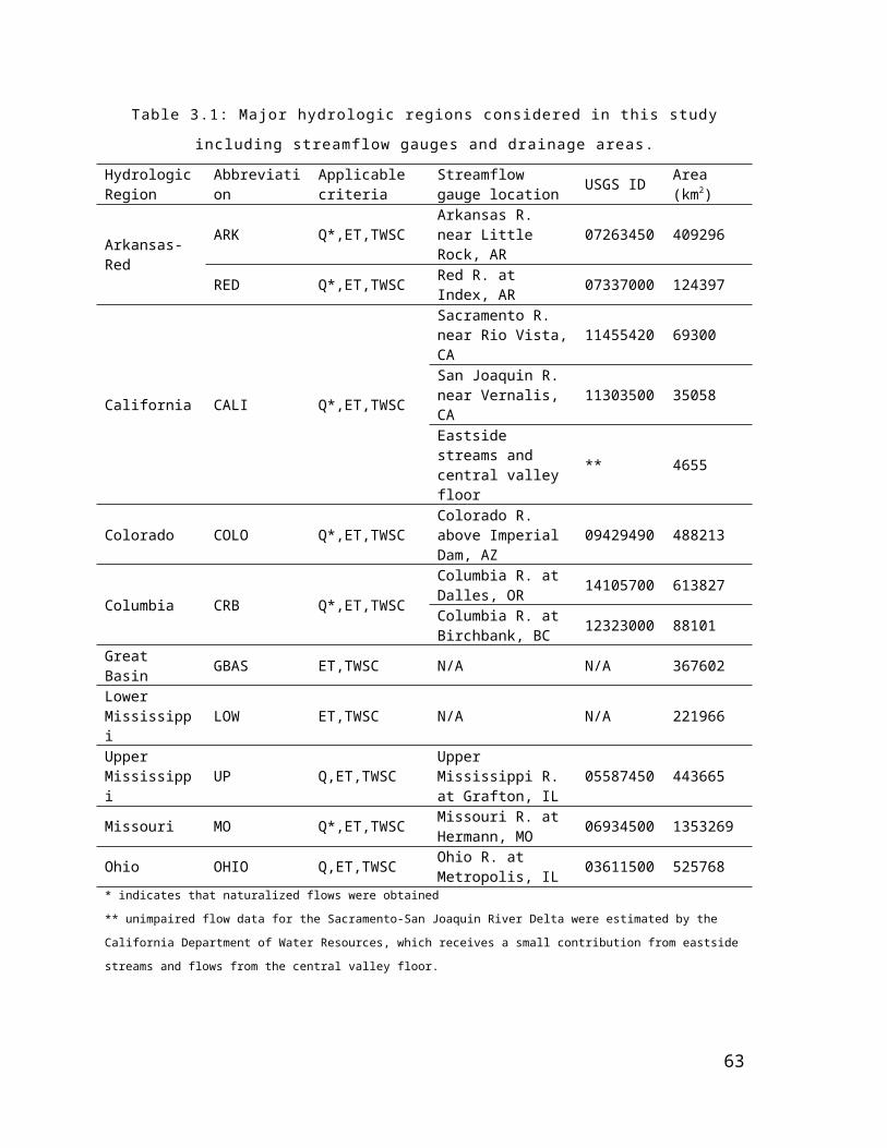
The Ohio River Basin is situated within a more uniform continental hydroclimatic regime
than the CRB. Its tributaries are more numerous (46, versus 9 in CRB) and hence represent
an even more comprehensive range of conditions specific to the region. The timing of
maximum and minimum flows is remarkably similar between the mean of the tributaries
and the major flows, consistent with the relative hydroclimatic homogeneity of the region.
Similar to CRB, the model under (over) predicted high (low) flows, while high correlation
among tributary streamflow is evident from their respective hydrographs. The smoother
simulated hydrographs at both scales is consistent with the overestimated persistence and
under estimated variance noted in Table 5.
Given the multiple data sets used in this study, it is essential to temper the findings with the
impact of overall data uncertainty. To train the model, several independent data sets were
used that could lead to offsetting errors across these datasets – i.e. ET versus TWSC –
highlighting potential water budget inconsistencies and data uncertainties. This is an
inherent potential pitfall in using independent datasets, however it may aid in ultimately
bracketing true conditions. One technique to reconcile such inconsistencies is through
redistributing the total water balance error from multiple sensors back to each of the
individual components using a Kalman error approach (Pan et al., 2011). This approach is
beyond the scope of this work; however it may offer a framework to further improve the
consistency of the remote sensing water budget analyses in the future.
Overall sources of error and uncertainty are as follows. TWSC uncertainties were perhaps
the largest within the study; evident in the disparity between mean monthly values from
individual processing streams in Figure 3.8. A further uncertainty arose in comparing these
data with ULM, given the different reference depths considered by each. ETAWB errors were
most likely to arise from the atmospheric components (left side of equation 1) that were
contingent upon the NARR analysis increment, particularly problematic over coastal
regions (Ruane, 2010); wherein adjustments to latent heating of the atmospheric column
are made to overcome moisture excesses in the underlying Eta model. ETSAT estimates were
subject to uncertainty from the input MODIS skin temperatures, which Ferguson et al.
(2010) described as being the largest source of error for a similar satellite-based ET
product, in lieu of errors associated with emissivity and land-surface characteristics.
Furthermore, the ETSAT estimates are not strictly constrained by moisture availability that
67

could lead to further data uncertainty. Q uncertainties due to random errors in the USGS
current meters or (for major basins) naturalization data and algorithms could skew the
interpretation of the model performance and trend analysis. Albeit, it is not immediately
apparent in which direction the skew would occur and it is expected – at least in the case of
the in-situ USGS data – that these errors would be small relative to the greater complexities
in the remote sensing data. Meteorological forcing errors may exist, particularly in regions
of topographical complexity. Most notably, precipitation errors would prevent the model
from matching streamflow timing, magnitude, and variability, while surface temperature
and wind errors could translate into erroneous estimates of surface water and energy fluxes.
Lastly, errors in model structure, or conceptualization errors may exist that ultimately
prevent the model from correctly simulating certain processes, or achieve the correct results
for the incorrect reason via calibration. Investigating these types of errors would require a
more directed and rigorous error analysis including detailed measurements of surface
fluxes of moisture and energy and their respective uncertainties.
3.5 Conclusions
We have exploited several observational data sets together with an LSM to estimate
various components of the terrestrial water budget. The analysis focused on ways to train
ULM to observational data sets to improve estimates of the water budget components. The
results were presented to provide insight into tradeoffs in the performance with respect to
each criterion. The single-best performing streamflow parameters for each basin were
utilized to streamflow variability and hydrologic response. Finally, an examination into
potential error sources was made to illustrate specific causes behind discrepancies in
simulated streamflows and their relationship across scale. The most important conclusions
of this analysis are:
1) Model calibrations towards a single-criterion had varied results. At large scales (≥ 105
km2) most basins were able to replicate Q, ET, and TWSC individually with reasonable
skill, despite uncertainties in the data themselves and discrepancies between modeled and
native retrieval resolutions. At 250 small-scale basins (< 104 km2) over daily time steps, ET
calibrations generally scored higher than Q, however for a small number of these, strong
disagreements between the model and remote-sensing product lead to ET simulations that
68

were poorer predictors than climatology, while Q calibrations always provided additional
skill
2) At large-scales, calibrations towards multiple-criteria had the best overall performance
when Q was included, followed by ETSAT, ETAWB, and TWSC. Altogether, calibrations
towards Q alone had the best all-around performance in terms of the other criteria, while
neither of the other criteria (ET, TWSC) alone or in combination was able to add
appreciable skill to Q prediction.
3) Multi-criteria performance at small scales followed similarly to the large-scale analysis
with the notable exception that the mutli-criteria calibration (Q and ETSAT together) out-
performed the single criterion Q-calibration in terms of Q performance at roughly one third
of the basins. This suggests that traditional streamflow calibration stands to benefit from
the inclusion of remote-sensing data.
4) The lack of a systematic bias in the satellite-ET product over a number of basins of
varying VI and Ts diversity indicates that above a certain threshold, VI-Ts diversity alone
may not be an adequate predictor of quality of the satellite-based ET product. Rather, the
issue of unbounded ET estimates during summer was most detrimental to the quality of ET
estimates.
5) The use of multiple criteria in the calibration procedure, at minimum serves to reduce
the equifinality problem when choosing the ‘best’ instance of the model parameters.
6) Investigating model error sources revealed that simulations generally under (over)
predicted high (low) flows. Comparing errors across scales also brought forth issues with
travel times and integrating differing hydroclimatic conditions across basins.
69
IV. REGIONAL PARAMETER ESTIMATION FOR THE UNIFIED LAND MODEL
This chapter is in review by Water Resources Research (Livneh and Lettenmaier, 2012).
4.1 IntroductionThe goal of parameter regionalization is to derive predictive relationships between
observable catchment descriptors and model parameters, and in so doing provide a basis for
a) avoiding time consuming local parameter estimation when a model is applied to a new
domain, and/or b) provide a basis for transferring parameters to ungauged basins. The most
common approaches for transferring parameter information in past work have been
multiple regression and interpolation (e.g. Magette et al., 1976, Karlinger et al., 1988, Post
and Jakeman, 1996, Abdulla and Lettenmaier, 1997, Kull and Feldman, 1998, Post et al.
1998, Post and Jakeman 1999, Fernandez et al. 2000, Merz and Bloschl 2004, Gan and
Burges, 2006, Heuvelmans, 2006, Wagener and Wheater, 2006, Boughton and Chiew,
2007, Goswani et al., 2007, Yadav et al., 2007, Viviroli et al., 2009) where the explanatory
variables are catchment characteristics. Other common techniques include hydrologic
classification and clustering methods (Vandewiele and Elias, 1995, Gupta et al., 1999,
Nijssen et al., 2001, Koren et al., 2003, Merz and Bloschl, 2004, Pokhrel et al., 2008,
Zhang et al., 2008), which essentially assign a priori model parameters to catchments either
via grouping into hydrologically homogenous regions, by relating parameters to land-cover
and climatic data, or by a combination of the two.
Singh et al. (2006) distinguish regionalization procedures for which site-by-site
model calibration is followed by regionalization, from those that perform calibration and
regionalization in a single combined step. Samaniego et al. (2010b) refer to the former as
postregionalization and the latter as simultaneous regionalization. The latter has the benefit
of incorporating additional geographical information (from nearby basins) into the
parameter estimation procedure. A few recent studies have implemented simultaneous
regionalization strategies, with varied results. Fernandez et al. (2000) attempted to optimize
regional relationships and regional model parameters simultaneously for 33 catchments in
70

the southeastern United States, and concluded that improvements in regional relationships
do not necessarily lead to improved model performance at ungauged sites. Kim and
Kaluarachchi (2008) compared a simultaneous calibration procedure with five
postregionalization techniques, and found modest improvements from the simultaneous
calibration. Hundecha and Bárdossy, (2004), Götzinger and Bárdossy, (2007), Pokhrel et
al. (2008) each had some success in simultaneous regionalization over different study
domains; however all found that parameter transferability was limited by the use of discrete
soil texture classes. Pokhrel et al. (2008) utilized the soil texture class relationships of
Koren et al. (2003) to constrain parameters during calibration. Samaniego et al., (2010a,b)
successfully applied a simultaneous regionalization procedure that considered the sub-grid
variability of catchment descriptors. This consideration has the advantage of enabling the
regionalization to incorporate information from finer resolution data to estimate effective
parameter values that are representative of the dominant hydrological processes at a coarser
grid and across scales.
Collectively, the range of explanatory variables that have been used in the aforementioned
studies include meteorological data (mean, variability and frequency information for
precipitation, temperature, potential evapotranspiration, solar exposure, and surface wind),
and land surface attributes (catchment geometry, aspect, and geomorphic data; geologic
information, soil fractional composition, texture classes, hydraulic properties and depth;
vegetation coverage, land-use information, and glaciation). Data sources have almost
entirely been in situ; to date, only limited use has been made of remote sensing data as
explanatory variables. In some cases, streamflow information has been used in
regionalization (e.g. baseflow index, peak discharge and recurrence, runoff ratio, specific
runoff), however this results in obvious limitations for parameter transfer to ungauged
basins.
Our major objective in this paper is to extend previous model development and calibration
efforts for the Unified Land Model (ULM – Livneh et al., 2011; Livneh et al., 2012a) to
improve model applicability to new domains. The model parameters that serve as the basis
for our regionalization relationships were derived through single and multi-criteria site-by-
site calibrations described by Livneh et al. (2012a). These calibrations involved minimizing
objective functions of errors between predicted streamflow, Q, and observations, as well as
71

in some cases, remote sensing estimates of evapotranspiration, ET. A secondary objective
of our work is to evaluate different methods for organizing catchment descriptors and
selecting model parameters to increase the quality of regional relationships and enhance
regional model performance.
Because there are many potential explanatory variables for regional parameter
estimation, and because many of these attributes are correlated by construct, we used a
principal components analysis (PCA) approach to maximize their explanatory skill and
minimize potential redundancy. This approach technically falls into the category of
‘postregionalization’, however in two experiments (described in Section 4.2.5) we
essentially retro-fit the data into a pseudo-simultaneous regionalization by conducting a
limited number of additional simulations – termed here as ‘zonalization’. This procedure
reevaluates the appropriateness of model parameter sets in the context of their performance
over neighboring catchments (i.e. in spatial zones). Similarities exist between zonalization
and other simultaneous regionalization approaches , but a key exception is that the
regionalization takes place a posteriori with respect to model calibration
We further test this approach in the context of global parameter transfer, by
restricting the regionalization procedure to only those catchment attributes with global
coverage. This provides a broader context for hydrologic modeling in data poor regions;
where stream gauges are not present, or for cases where site specific calibration is not
computationally viable.
4.2 MethodsWe describe in this section the ULM model and its parameters, along with the
geospatial and hydrometeorological data needed to set-up and force the model. We also
summarize the structure of the regionalization experiments, and the form of PCA and bias
correction techniques used.
4.2.1 Study area and data sourcesThe study domain consists of 220 river basins with drainage areas in the range 102 – 104
km2 distributed across the CONUS (Figure 4.1). The 220 basins were selected to provide a
broad cross section of hydroclimatic regimes (see Livneh et al., 2012a for details). The
catchments are a subset of the MOdel Parameter Estimation EXperiment (MOPEX) data
72

set (Schaake et al., 2006) which has been screened to assure an adequate density of
precipitation gauges and minimal effects of upstream anthropogenic activities such as
irrigation diversion and reservoir operations. Streamflow data were obtained directly from
United States Geologic Survey (USGS) archives.
Figure 4.1: Map of the study domain, including 220 basins (yellow) and location of precipitation gages used in the forcing data set (fine black dots).
4.2.2 Model forcing dataThe meteorological forcing data used in this study were derived by Livneh et al. (2012b)
and are available at a 1/16° resolution over the CONUS domain for the period 1915 – 2010.
The gridded precipitation and daily minimum and maximum temperatures are based on a
total of approximately 20,000 NOAA Cooperative Observer (Co-op) stations shown in
Figure 4.1. Wind data were linearly interpolated from a coarser (1.9° grid) NCEP–NCAR
reanalysis grid (Kalnay et al. 1996), which also was used to produce a daily wind
climatology for years prior to 1948.
4.2.3 Catchment attribute dataThe catchment attribute data sets are summarized in Table 4.1 and serve as candidate
predictor variables for the regionalization experiments. The first set of attributes
correspond to the soil texture class relationships used by Koren et al. (2003) to estimate a
set of a priori model parameters for the NWS Sacramento model (Sac). These soil
parameters are specific to the Sac model, which is the basis for the soil hydrology in ULM.
73

The soil texture relationships used by Koren et al, (2003) are readily estimated from
STATSGO data (Schwarz and Alexander, 1995), and heretofore represent the default
parameters for ULM.
The second set of catchment attributes includes the remaining land-surface characteristics
that can be derived from inputs required by ULM. These include geomorphic variables
(derived from the input DEM), vegetation information such as percent forest cover and
seasonal greenness, as well as information pertaining to soil temperature climatology and
seasonal land-surface albedo. The third set of attributes is derived from two remote sensing
moisture flux products that are described in detail by Livneh et al. (2012a). These include
the MODIS-based ET data product of Tang et al. (2009), as well as terrestrial water storage
change (TWSC) based on Gravity Recovery and Climate Experiment (GRACE) data. Since
the GRACE data are at coarser resolution (~1°) than the model spatial resolution (1/16°),
we compute a spatially weighted average TWSC value for each basin. The final set of
attributes are taken from the GAGES-II data set, which includes information about basin
morphology, climate, topography, soils, anthropogenic disturbance factors, as well as land
use. Only floating-point basin attribute data in GAGES-II were considered. Also, we did
not consider streamflow-based attributes, since these are not available for ungauged basins.
74

Table 4.1: Catchment attributes used as candidate explanatory variables in parameter
regionalization.
Soil texture attributes Description ReferenceTension and free water storages, hydraulic conductivities, impervious areas, percolation constant, recession slope.
a priori values from soil texture relationships
Koren et al. (2003), Schwarz and Alexander (1995)
Geomorphic attributesBasin area, mean elevation, maximum relief, approx. length of main stream, relief ratio, shape factor, length-to-width ratio, elongation ratio
Defined from DEM and USGS GIS HUC 250K database
Seaber et al. (1987)
Land surface characteristic attributesPercentage of basin covered in forest; Satellite-based greenness fraction and albedo – monthly, seasonal, annual means, standard deviations, minimums, and maximums
Required as inputs into ULM
Gutman and Ignatov(1998)
Remote sensing attributesEvapotranspiration – monthly, seasonal, annual means, standard deviations, minima, and maxima
Derived entirely from satellite data (MODIS, SRB)
Tang et al. (2009)
TWSC – monthly, seasonal, annual means, standard deviations, minima, and maxima
GRACE data, mean of 3 processing streams*
Swenson and Wahr (2006)
Meteorological attributesPrecipitation, Temperature, Wind – monthly, seasonal, annual means, standard deviations, minima, and maxima
Derived from station co-op data and reanalysis fields (wind only)
Livneh et al. (2012a)
GAGES-II attributesSoils data, climatic, land-use, morphology transitionary data, population density, drainage density classes, and anthropogenic disturbance factors
A single basin-average value for each field, only floating point data considered (i.e. no integer class data)
Falcone et al. (2010)
4.2.4 Land surface modelULM is a merger of the land surface components from the Noah land surface model
(LSM; Ek et al., 2003) – e.g., vegetation, ET computation, snow model, and algorithms for
computing frozen soil, surface heat and radiative fluxes – and subsurface elements (soil
moisture and runoff generation algorithms, as well as infiltration) from the NWS
Sacramento Model (Burnash et al., 1973). The snow model is described by Livneh et al.
(2010). It is essentially the standard Noah snow model augmented to include time-varying
75

albedo, partial snow cover, and retention of liquid water within the snowpack. Livneh et al.
(2011) evaluated ULM performance with respect to observed river discharge, flux towers
measurements of surface heat fluxes, and soil moisture. Table 4.2 summarizes plausible
physical ranges of the model soil parameters that constrained the parameter estimation
here.Table 4.2: List of ULM soil parameters from NWS Sacramento Model and their plausible
ranges.
Parameters Unit Description Plausible RangeUZTWM mm Upper zone tension water maximum storage 1.0 - 300UZFWM mm Upper zone free water maximum storage 1.0 - 300UZK day-1 Upper zone free water lateral depletion rate 0.05 – 0.75ZPERC - Maximum percolation rate 1.0 - 350REXP - Exponent of the percolation curve equation 0.0 – 5.0LZTWM mm Lower zone tension water maximum storage 1.0 - 500
LZFSM mm Lower zone free water supplemental maximum storage 1.0 – 1000
LZFPM mm Lower zone free water primary maximum storage 1.0 – 1000
LZSK day-1 Depletion rate of the lower zone supplemental free water storage 0.01 – 0.8
LZPK day-1 Depletion rate of the lower zone primary free water storage 0.0001 – 0.025
PFREE - Percolation fraction going directly from upper zone to lower zone free water storages 0.0 – 0.8
PCTIM - Impervious fraction of the ground surface 0.0 – 0.1
ADIMP - Maximum fraction of additional impervious area caused by saturation 0.0 – 0.45
4.2.5 Regionalization procedureThe regionalization approach seeks to leverage the site-by-site calibrations
performed by Livneh et al. (2012a). In that work, each basin underwent a multi-objective
calibration involving approximately 2000 simulations per basin, from which a set of
Pareto-optimal parameter sets, θP, was identified which minimize streamflow prediction
errors. Given the large inherent data-storage requirements, only summary data from these
calibrations were retained for each basin; these consist of the roughly 2000 parameter sets
and their associated performance statistics. The major performance statistics used were the
components of the Nash-Sutcliffe coefficient (NSE – Nash and Sutcliffe, 1970) pertaining
to differences in simulated and observed streamflows (Gupta et al., 2009). These include
76
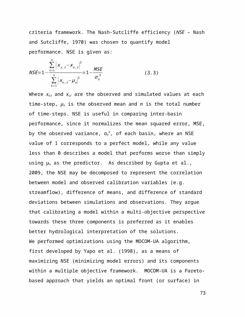
the Pearson correlation coefficient, R, the difference in mean flows, α, and the difference in
standard deviations, or range-shift, β . An important point here is that when calibrating the
three components of the NSE in a multi-objective context, the resulting Pareto set of
solutions have statistics that are non-dominant with respect to each other (i.e. there are
tradeoffs between R, α, β). However, Livneh et al. (2012a) observed that the effective NSE
for these parameter sets are not necessarily equal, and some sets may have slightly higher
or lower NSE than others.
The pairs of parameter sets and performance statistics from Livneh et al. (2012a)
were reanalyzed in 2 ways that address the findings of previous regionalizations (e.g.
Fernandez et al., 2000) detailed in section 4.1. The assertion of that work is that a strong
predictive relationship between catchment descriptors (predictors) and calibrated model
parameters (predictands) will not necessarily lead to improved model performance using
regionalized parameters. Therefore we designed four experiments to test the impact of
predictive relationship strength on regionalized model performance by selecting
predictands and predictors in several ways that alter the predictive relationships. The
predictive relationship between each predictor/predictand set was derived using PCA
(described in section 4.2.6) and the resulting ULM performance using regionalized model
parameters was compared for each experiment. The first two experiments (Table 4.3)
contrast parameter selection (predictands), based on either local or zonal
representativeness, illustrated in Figure 4.2. Local parameters were selected based on the
NSE for the basin of interest, whereas zonal parameters were selected based on the average
NSE that resulted from iteratively simulating each Pareto-optimal parameter set, θP, from
the basin of interest, at its neighboring basins (which we defined as being all basins for
which the gauge was within a 5° latitude-longitude of the target basin gauge). The first
experiment used locally optimized parameters, θP-LOCAL, and thus followed a classic post-
regionalization approach, where a predictive relationship was derived between local
catchment descriptors and locally optimized model parameters. In the second experiment,
we zonalized the model parameters prior to regionalization, (i.e. θP-ZONAL), which is
anticipated to produce more spatially representative model parameters and test the assertion
above. The third and fourth experiments were similar to the first two experiments, except
77

that the zonal procedure was extended to the catchment descriptors, η, with each basin’s
catchment descriptors (ηLOCAL) replaced by their mean values within a 5° radius (ηZONAL).
Figure 4.2: Flow chart illustrating the procedure for selecting locally and zonally optimized model parameters based on ranking Nash-Sutcliffe efficiency (NSE) from Pareto-optimal parameter sets that were non-dominant in terms of Pearson correlation, R, difference in means, α, and difference in standard deviation, β.
78

Table 4.3: Regionalization experiments considering either local or zonal predictands (ULM
parameters, θP) and predictors (catchment attributes, η).
ULM parameters (predictands)θP-LOCAL θP-ZONAL
Catchment attributes
(predictors)
ηLOCAL Experiment 1 Experiment 2
ηZONAL Experiment 3 Experiment 4
4.2.6 Principal Components Analysis (PCA)PCA was used to develop predictive relationships between catchment descriptors
and model parameters for each experiment listed in Table 4.3. Garen (1992) developed a
PCA regression procedure to improve streamflow volume forecasting that included a
systematic search for optimal or near-optimal combinations of variables. The procedure has
since been used in numerous studies for applications related to hydrologic data
reconstruction, reservoir modeling, and water supply forecasting (e.g. Hidalgo et al., 2000,
Rosenberg et al., 2011). Hidalgo et al. (2000) found this method to produce more
parsimonious results than other PCA-regression based models. To date, this method has not
been used specifically for LSM parameter regionalization, although the method is suitable
for incorporating a large number of predictor variables (i.e. candidate catchment attributes).
Therefore, we applied the Garen (1992) approach as implemented by Rosenberg et al.
(2011) with the exception that we considered all descriptors with non-zero correlations
with the model parameters (as opposed to considering only positively correlated descriptors
as is typically done). The procedure includes an iterative series of t-tests between
catchment attributes and model parameters, ultimately preserving only those principal
components (i.e. combinations of descriptors) that are statistically significant (α = 0.1). A
jack-knifing approach was used to predict parameter values for each basin based on its
catchment descriptors, such that the predictive equation is derived exclusively from
information from the other basins. This procedure was chosen to emulate the prediction of
model parameters for ungauged basins.
79

4.3 Results and discussionWe evaluated the variability and spatial coherence of the regionalization input data,
followed by an examination of the tradeoffs in model performance that result from using
locally versus zonally optimized inputs (θ and η). We then compared ULM performance
from all regionalization experiments to understand which strategy produces the best results.
4.3.1 Spatial CoherenceFigure 4.3 shows the inputs to the four regionalization experiments. The western
U.S. is enlarged to illustrate the spatial coherence of zonal model parameters. Livneh et al.
(2011) found ULM to be highly sensitive to the parameter shown in Figure 4.3 (UZTWM).
This suggests that model parameters chosen on the basis of zonal performance indeed have
detectable spatial coherence and may be linked to processes with length scales larger than
those of an individual basin. This is an encouraging preliminary result, given that our
ultimate goal is to find a set of regional equations that describe model parameter variations
across large spatial scales.
Figure 4.3: Example illustrating the spatial coherence of a set of candidate inputs for the regionalization experiments, which regionalize predictors (catchment attributes) and predictands (ULM parameters) that were selected either zonally or locally (e.g. Exp. 1 uses local predictands and local predictors as inputs to the PCA regionalization, see Table 4.3 for other experiments). The western U.S. is enlarged to show the spatial coherence of the zonal parameter value, UZTWM.
80
One way to quantify the coherence of a phenomenon in space (parameter
variability) is by constructing an experimental variogram, γ¿ ( H k ). This provides a measure
of the average dissimilarity of a vector class, ℌk, as a function of distance, h, by computing
the dissimilarity between all pairs of samples within a region, i.e.:
γ¿ ( H k )= 12nc
∑α=1
nc
( z ( xα+h )−z ( xα ) )2 (4.1)
Where z(xα) represents a parameter value in space for all samples, nc. The experimental
variogram is typically computed using vectors, h, of a length less than half the diameter of
the region (Wackernagel, 2003). The experimental variograms for the locally optimized
and zonally optimized parameters are shown in Figure 4.4. For ease of viewing
dissimilarities, were binned by 1° intervals, and dissimilarities were normalized by the
square of the mean of each parameter value to facilitate inter-parameter comparison. Two
important variogram features are apparent. The first is the dissimilarity value in the bin
closest to the origin, which denotes how abruptly the values of the variable changes at a
very small scale. This is called the nugget-effect, which draws its name from the field of
gold mineral exploration. The second important feature of the variogram, the sill, is the
distance beyond which increases in variability become negligible. This distance is called
the range, and essentially represents the length scale of spatial coherence for a given
parameter.
81
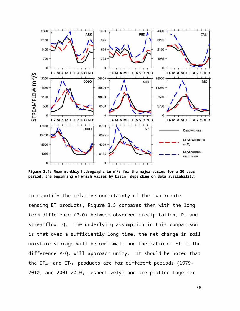
Figure 4.4: Experimental variograms for both zonal and local model parameters, illustrating greater spatial coherence for zonal parameters shown. Only those parameters with a detectable range are included, which is consistently present for zonal parameters.
Figure 4.4 shows only those parameters with a range that could be detected
graphically. In all cases, the zonally optimized parameters have ranges that are greater than
those of the locally optimized parameters and in some cases no sill was detected for locally
optimized parameters, whereas one was for zonal optimizations. Although this should
follow for all zonally optimized parameters by construct, roughly half of the parameters did
not have detectable ranges, which may indicate that model performance is not very
sensitive to their values, or alternatively that parameter values may be correlated with fields
that are not spatially coherent. The cases where no sill was detected for locally optimized
parameters (while one was in fact detected for zonal optimization) were for instances of
small spatial coherence, where the range was entirely contained within the 5° zoning
window (for parameters LZTWM, LZFSM, REXP). This suggests that the size of the
82

selected zoning window (5°) could impact the extent of the range. The presence of the
nugget effect for all parameters indicates considerable variability even at very small scales.
The nugget-effect is frequently smaller in zonal than local parameters, but not always,
which is likely caused by the combination of parameter uncertainty and model streamflow
prediction errors (i.e. imperfect optimizations). Overall, the parameters with detectable
ranges in Figure 4.4, especially ADIMP and UZTWM, are consistent with those identified
by Livneh et al. (2011) to which ULM was most sensitive.
4.3.2 Simulated streamflow performanceThe tradeoffs in model performance associated with using zonal as contrasted with
locally optimized parameters are shown in Figure 4.5. For approximately 20% of the
basins, the best zonal performance resulted from the best locally optimized parameters –
i.e. zonal and local parameters produced essentially the same result. For the remaining
~80% of basins, Figure 4.5 shows that the penalty for using zonal parameters for a given
basin (i.e. locally) is comparatively smaller than the penalty for using local parameters
zonally. Rohini and Samaniego (2011) found an analogous result for an LSM calibrated
over a number of basins in Germany, with the aim of not over-fitting parameters to an
individual basin. We infer from these results that model performance using zonalized
parameters has a comparatively smaller penalty than local optimization, while lessening the
degree of over-fitting parameters to any single basin.
83

Figure 4.5: Illustration of tradeoffs in model performance when running (a) zonal parameters (θP-ZONAL) locally and (b) running local parameters (θP-LOCAL) zonally (averaged NSE over a 5° latitude-longitude window – see Figure 4.2 for definitions). The solid-black line was drawn connecting ranked Nash-Sutcliffe Efficiency (NSE) for 220 basins and represents the upper-envelope for model performance, either locally (a), or zonally (b), while the thin gray lines show that the penalty in local performance for using θP-ZONAL is much smaller than the penalty in zonal performance using θP-LOCAL..
Figure 4.6 compares skill scores from the four regionalization experiments to local
optimization. Differences in skill vary between regionalization experiments; however skill
scores tend to be lowest relative to local calibration for basins where local optimization was
itself the least skillful (i.e. on the right-most tail of the plots). An interesting result is that
for several cases, the regionalized model outperformed the local optimization – most
frequently for the case of zonalized parameters with local catchment descriptors. The
complete results from the calibration period (1991-2010) and a validation period of equal
length (1971-1990) are tabulated in Table 4.4. For both time periods, regionalization using
zonal rather than locally optimized parameters scored slightly higher, while the opposite
84

was true for catchment descriptors – experiments using local (zonal) catchment descriptors
had slightly higher (lower) skill. This finding supports a hypothesis that model parameters
may in fact be zonally representative, given their function of integrating model physics
with hydro-meteorological processes. These processes frequently have length-scales larger
than an individual catchment (e.g. seasonal frontal precipitation over the central and eastern
U.S.). Alternatively, catchment descriptors generally represent spatially-fixed local
phenomena that are not necessarily well-expressed through areal averaging. However, it is
worth noting that the spatially averaged zonal catchment descriptors were not a direct
analogue to the zonal parameters, which were selected following a non-linear
transformation through ULM and a subsequent streamflow comparison.
85

Figure 4.6: Comparison of the four regionalization experiments with local optimizations. The solid black line represents the NSE of each basin (ranked) as in Figure 4.5a, whereas the colored lines show regionalized model skill (ULMR) for each experiment. The first word in the panel labels refers to which parameters, θ , were used, while the second refers to the catchment descriptors, η, such that, for example, “ZONAL-LOCAL” represents the regionalization using zonal model parameters with local catchment descriptors.
86

Table 4.4: Model performance (in terms of NSE) for calibrations and regionalization
experiments.
Simulation type Calibration Period Validation PeriodMean Std. deviation Mean Std. deviation
Locally Optimized 0.5385 0.5662 0.5228 0.5526Zonally Optimized 0.5183 0.5467 0.4489 0.4898
θP-ZONAL -ηZONALRegionalization 0.4350 0.4842 0.4455 0.4855θP-ZONAL -ηLOCALRegionalization 0.4385 0.4903 0.4466 0.4847θP-LOCAL -ηZONALRegionalization 0.4164 0.4714 0.4286 0.4747θP-LOCAL -ηLOCALRegionalization 0.4309 0.4854 0.4389 0.4802
The validation period is useful as a test of the robustness of model parameters and is
important for model studies dealing with hydroclimatic sensitivities. Both the locally and
zonally optimized skill scores are smaller during the validation period than in the original
period used for parameter estimation, but the drop for zonally optimized parameters is
more marked. Somewhat surprisingly, model skill from the regionalization experiments
was slightly higher in the validation period than in the calibration period from which their
predictive relationships were derived. Despite the differences in model skill between the
two time periods, a paired t-test was performed which showed that none of the differences
listed in Table 4.4 was statistically significant.
4.3.3 Principal components and catchment descriptorsThe final equations used to predict model parameters were made up of
combinations of statistically significant principal components (PCs), which themselves
were composed of catchment descriptors. Table 4.5 summarizes the number of catchment
descriptors, PCs, and the PCA parameter prediction errors, expressed as a normalized
standard error:
SE= s/√nθ
(4.2)
Where s is the standard deviation of parameter estimation errors, n is the number of basins,
and θ is the mean value of the parameter being estimated. The number of PCs needed to
estimate a given parameter varied from 1 to 26, with an average of approximately 10, while
the number of catchment descriptors used in estimation ranged from 17 to 47 with an
average of 27. Quantitatively, these numbers did not appear to have an impact on the
overall quality of parameter estimates. The θP-ZONAL-ηLOCAL regionalization had the smallest
87
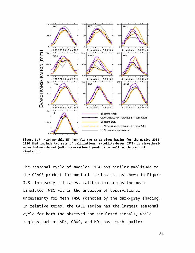
parameter prediction error and the best regionalized model performance. The predictive
errors and regionalized model performance from the other experiments intuitively followed
similarly. Therefore, although it was called into question by Fernandez et al. (2000), this
conclusion appears to hold in this case, namely higher quality regionalization relationships
ultimately produce better model simulations. Table 4.5: Counts of principal components and catchment descriptors needed to for the
predictive equations for each model parameter listed below; normalized standard error
(Equation 4.2) was computed from the differences between the predictand (either θ P -L O C AL , or
θP -Z O NA L) and the PCA generated estimated value for each regionalization experiments, where
the first letter in the heading refers to parameter optimization, θ P ,, and the second refers to
the catchment attribute, η – i.e. Z=”zonal”, L=”local”.
Principal Components Catchment DescriptorsNormalized Standard Error, SE
Experiment LL LZ ZL ZZ LL LZ ZL ZZ LL LZ ZL ZZ
UZTWM 19 15 17 20 28 52 31 35 0.421 0.456 0.391 0.373
UZFWM 9 9 12 13 37 44 28 27 0.567 0.566 0.530 0.548
LZTWM 11 7 10 8 43 24 22 30 0.523 0.539 0.537 0.552
LZFPM 20 15 26 14 28 27 40 22 0.432 0.514 0.369 0.426
LZFSM 16 9 12 10 36 28 34 33 0.522 0.572 0.468 0.529
UZK 7 9 11 7 33 31 36 29 0.614 0.608 0.543 0.578
LZSK 21 18 22 17 31 26 32 34 0.326 0.395 0.322 0.370
LZPK 8 6 10 10 44 23 28 24 0.520 0.525 0.502 0.502
ADIMP 22 16 23 26 31 24 35 44 0.868 0.925 0.735 0.740
PCTIM 11 9 22 13 27 17 45 32 0.847 0.871 0.727 0.817
REXP 11 7 8 5 28 31 28 27 0.607 0.643 0.619 0.645
PFREE 11 4 8 1 25 24 32 17 0.544 0.581 0.578 0.631
ZPERC 13 7 7 5 47 26 30 27 0.450 0.470 0.501 0.498
Mean 11.93 8.73 12.53 9.93 29.2 25.13 28.07 25.4 0.483 0.511 0.455 0.481
Table 4.6 shows the overall frequency and use of descriptor variables in terms of
their respective classes. Descriptors from the GAGES-II database far outnumber all others,
and were also used most frequently for parameter predictions. The next most frequently
used attributes were the GRACE-based TWSC, which were used nearly twice as often as
the other remote sensing data set (ET), which was least frequently used overall.
88

Table 4.6: Summary of catchment descriptors used in regionalization, including the average
number of parameters each descriptor was used to predict (frequency), and the total number
of descriptors used from each class.
Descriptor classMean frequency of descriptor-class in
predictions
Fraction of descriptors used
(from total)Soil texture 2.0 9/19Geomorphic 2.5 8/8
Meteorological 2.1 10/16ET 1.4 7/8
TWSC 2.6 5/8GAGES-II 2.8 274/313Mean total 2.23 313/372
Table 4.7 provides insights into the most explanatory catchment descriptors for
each parameter in the regionalization process; computed as the product of the descriptor
coefficient (in its respective PCs) and the mean descriptor value across all catchments (θ).
Every category of catchment attributes (summarized in Table 4.2) was represented within
the most significant set of descriptors shown in Table 4.7. Somewhat surprisingly, soil-
based attributes were not ubiquitously among the most explanatory descriptors, and were
not among the three most predictive descriptors for the lower zone soil moisture storage
parameters (LZFSM, LZFPM). Also noteworthy was the frequent occurrence of
temperature-related descriptors, which may reflect their connection to radiation and the
ensuing effect on model ET. Similarly, relative humidity and remote-sensing ET were
found to be significant descriptors for several cases. A notably intuitive relationship
resulted between a related descriptor and parameter, namely the topographical wetness
index and the parameter ADIMP, which represents the maximum fraction of additional
impervious area caused by saturation. Finally, several a priori ULM parameters (from the
Koren et al., 2003 Sacramento Model parameter estimation) were found to be explanatory
predictors. Somewhat unexpectedly, the explanatory a priori predictors were not of the
same parameter. This can be partially reconciled by the fact the a priori parameters
themselves were derived from the same soils data base (STATSGO) and they frequently
represent inter-related processes. An example is the a priori value of PFREE (representing
the percolation fraction going directly from upper zone to lower zone free water storages)
that was an explanatory descriptor for REXP (the exponent of the percolation curve
89
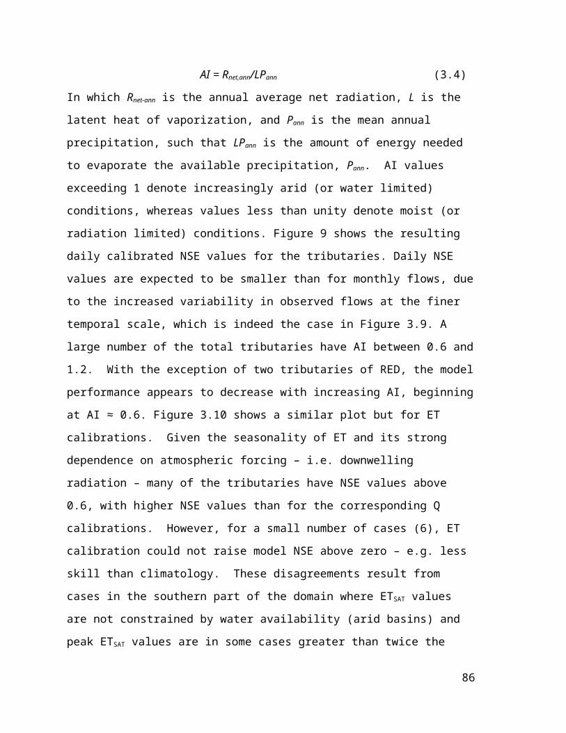
equation), which are both computed from the estimated soil wilting point in the original
derivation of Koren et al. (2003).
90
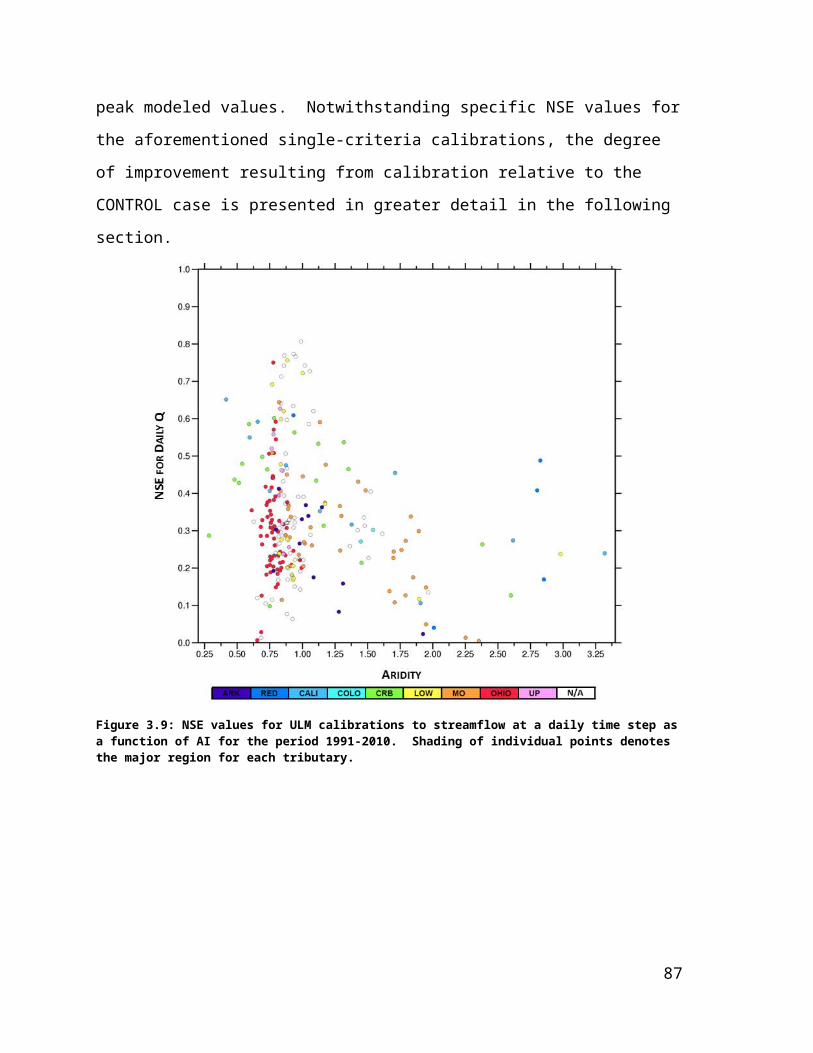
Table 4.7: The three most explanatory catchment descriptors for each predicted model
parameter, based on the product of the regression coefficients and the mean descriptor value
(all descriptors below were part of statistically significant PCs in the prediction equations).
For each parameter the descriptors are listed in order of their explanatory strength. Results
are shown only for the case of zonal parameters with local descriptors
Parameter Catchment descriptor Explanation Source
UZTWMmax_inter-monthly_tmin Maximum inter-monthly daily minimum temperature Met. Datamax_inter-monthly_tmax Maximum inter-monthly daily maximum temperature Met. DataCLAYAVE Average value of clay content (percentage) GAGES-II
UZFWM
RH_BASIN Watershed average relative humidity (percent) GAGES-II
ZPERC A priori value of maximum percolation rate coefficient Koren et al. (2003)
NO4AVE Average value of percent by weight of soil material less than 3 inches in size and passing a No. 4 sieve (5 mm) GAGES-II
LZTWM
BAS_COMPACTNESS Watershed compactness ratio, = area/perimeter2 Geomorph.
HGBPercentage of soils in hydrologic group B. Hydrologic group B soils have moderate infiltration rates. Soils are moderately deep, moderately well drained, and moderately coarse in texture.
GAGES-II
max_inter-monthly_tmin Maximum inter-monthly daily minimum temperature Met. Data
LZFPMAPR_TMP7100_DEGC Average April air temperature for the watershed (degrees C) GAGES-IImean_monthly_greenness Mean monthly value of basin-wide greenness fraction Land. surf.T_MIN_BASIN Watershed average of minimum monthly air temperature (degrees C) GAGES-II
LZFSM
RH_BASIN Watershed average relative humidity (percent) GAGES-IIMAM_albedo Average seasonal basin-wide albedo (Mar., Apr., May) Land. surf.
MAINSTEM_SINUOUSITYSinuosity of mainstem stream line. Defined as curvilinear length of the mainstem stream line divided by the straight-line distance between the end points of the line.
GAGES-II
UZK
MAY_PPT7100_CM Mean May precip (cm) for the watershed GAGES-II
MAINS800_21 Mainstem 800m buffer "urban", 2001 era. Sum of MAINS800_21, 22, 23, and 24. Buffer is the area 800m each side of stream centerline GAGES-II
maxInterTWSC Maximum inter-monthly terrestrial water storage change Remote sens.
LZSK
MAM_greennnes Average spring basin-wide greenness fraction (Mar., Apr., May) Land. surf.sd_monthly_albedo Standard deviation of monthly albedo Land. surf.
NO200AVE Average value of percent by weight of soil material less than 3 inches in size and passing a No. 200 sieve (.074 mm) GAGES-II
LZPKWDMAX_BASIN Watershed average of monthly maximum number of days (days) of
measurable precipitation GAGES-II
BAS_COMPACTNESS Watershed compactness ratio, = area/perimeter2 GAGES-IISON_greennness Average autumn basin-wide greenness fraction (Sept., Oct., Nov.) Land. surf.
ADIMPTOPWET Topographic wetness index GAGES-IImax_inter-monthly_tmax Maximum inter-monthly daily maximum temperature Met.RIP800_52 Riparian 800m buffer percent Shrubland GAGES-II
PCTIMLST32F_BASIN Watershed average of mean day of the year (1-365) of last freeze GAGES-IIMAM_albedo Average seasonal basin-wide albedo (Mar., Apr., May) Land. surf.T_MAX_BASIN Watershed average of minimum monthly air temperature (degrees C) GAGES-II
REXP
PCT_2ND_ORDER Percent of stream lengths in the watershed which are second-order streams (Strahler order); from NHDPlus GAGES-II
PFREE Apriori value of percolation fraction going directly from upper zone to lower zone free water storages
Koren et al. (2003)
ROADS_KM_SQ_KM Road density, km of roads per watershed sq km, from Census 2000 TIGER roads GAGES-II
PFREE
UZTWM Apriori value of upper zone tension water capacity Koren et al. (2003)
LZTWM Apriori value of lower zone tension water capacity Koren et al. (2003)
S4ET Mean evapotranspiration in autumn (September, October, November) Remote sens.ZPERC elongation_ratio Diameter of a circle with basin area divided by the maximum transect. Geomorph.
91

PCT_3RD_ORDER Percent of stream lengths in the watershed which are third-order streams (Strahler order); GAGES-II
4.3.4 Global parameter estimation experimentTo emulate parameter estimation in data-poor regions, we repeated the most
effective regionalization from section 4.3.2 (θP-ZONAL-ηLOCAL) as well as the classic
postregionalization (θP-LOCAL-ηLOCAL) using only globally available catchment attributes. The
two experiments chosen represent the recommended and conventional regionalizations,
respectively. They exclude the GAGES-II attributes (which comprised a large number of
explanatory catchment descriptors in each original experiment, but are available only for
the CONUS). The total number of candidate catchment attributes was reduced to 65 for
these tests. Figure 4.7 compares ULM performance as for Figure 4.6, however, with the
addition of the global coverage experiments. Both of the global experiments perform
remarkably closely to the experiments in section 4.3.2 with very modest reductions in both
mean and standard deviation of the skill scores (NSE listed on Figure 4.7).
92
Figure 4.7: Comparison of ULM using locally optimized parameters with the original regionalization experiments (ULMR, section 4.3.2) and the global experiments (ULMRG, section 4.3.4). The mean NSE for all basins for ULMRG were only slight reduced from the values listed in Table 4.4.
In the absence of GAGES-II catchment attributes, the PCA procedure identified
alternative explanatory catchment attributes in place of those used in the original
experiments (i.e. described in Table 4.7). Some of the most apparent replacements (not
tabulated) for ULM-sensitive parameters (as identified by the experimental variograms)
were: topographic wetness index was replaced by soil porosity for ADIMP; average clay
content was replaced by mean monthly precipitation for UZTWM; and mean monthly
temperature replaced relative humidity for LZFSM . Meanwhile the most explanatory
descriptors for PFREE remained unchanged. Altogether, in the absence of GAGES-II data,
the PCA procedure was robust in preserving much of the explanatory information to
estimate ULM parameters.
93

4.4 Summary and conclusionsWe have described a methodology for regionalizing ULM parameters based on a set
of parameter optimizations and ancillary (predictor) variables for 220 catchments located
across the CONUS. Both local and zonal parameterization approaches were developed, and
were evaluated in a series of regionalization experiments that ultimately compared the
impact of initial parameter and catchment attribute selection on regionalized model
performance. A PCA approach constructed predictive relationships between locally or
zonally optimized model parameters and PCs consisting of catchment attribute variables
that include soil texture, geomorphic, meteorological, and land surface features, as well as
two remote sensing data sources and the GAGES-II data set. Our main conclusions are:
1. The penalty in streamflow prediction skill for using zonal parameters at an
individual basin (i.e. locally) is comparatively smaller than the penalty for using
local parameters zonally. This suggests that it is possible to avoid over-fitting model
parameters to individual basins, while preserving a significant amount of predictive
skill.
2. The experiments showed that the quality of regionalized model performance is
directly related to the strength of parameter predictive relationships. Therefore, to
be most effective, future regionalization efforts should seek ways to pair model
parameters (predictands) and catchment (attributes) prior to regionalization (as done
here through zonalization) to further improve regionalization quality.
3. Over the 20-year training and validation periods, the most skillful model
performance resulted from regionalizations that used zonal model parameters and
local catchment descriptors as inputs for the PCA procedure. Both the calibrated
and regionalized parameter sets were temporally robust, since differences in
performance between the training and validation periods were not statistically
significant.
4. The approach worked surprisingly well when only globally available data sources
were used. Although many of the best predictors in the original experiment were
from the GAGES-II data set (which is only available for CONUS), other parameters
displaced those based on GAGES-II, with little loss in accuracy.
94

Acknowledgements
The work on which this paper is based was supported by NOAA Grant No.
NA070AR4310210 to the University of Washington. This work was facilitated through the
use of advanced computational, storage, and networking infrastructure provided by the
Hyak supercomputer system, supported in part by the University of Washington eScience
Institute. We appreciate the advice of Mr. Eric Rosenberg in implementing the PCA
method, and of Dr. Bart Nijssen for discussions related to the experimental design.
95

V. CONCLUSIONS
The research reported in this dissertation addresses the four science questions from Chapter
I, specifically: (i) Which ULM structures produce the most realistic simulations of surface
hydrology and land-atmosphere interactions?, (ii) How well can the ULM structures be
used to accurately estimate the terrestrial water balance at both catchment and regional
scales?, (iii) Can the use of ground-based and satellite observations provide a physically
consistent framework from which to derive model parameters that result in realistic water
balance estimates?, and (iv) To what extent can parameter information from ULM
simulations (102 – 104 km2) be transferred to other catchments through predictive
relationships derived exclusively from directly observable catchment attributes? The
development and implementation of the model took place in three stages that first
addressed model structure, followed by model parameters, and finished with model
regionalization.
The initial objective of the model development effort was to evaluate the potential
of ULM to improve weaknesses of its parent models, Noah and Sac, while taking
advantage of their respective strengths. It was shown that ULM more accurately simulates
the soil drying cycle than does Noah, which has implications for drought monitoring
applications. The improvements in hydrology did not hinder surface heat flux estimates,
which were similar or modestly superior to Noah. This is relevant to coupled land-
atmosphere applications (i.e., numerical weather prediction) and is significant in a
benchmarking context, which implies that updates to one aspect of model physics need not
come at the expense of another. In order to adequately capture streamflow dynamics,
limited parameter tuning was needed. One key finding is that there is a need for a
representative set of ULM parameters, and that simply utilizing native Sac soil parameters
within the ULM structure does not necessarily lead to realistic model responses.
Another goal of this dissertation was to incorporate in situ and remote sensing
observations of the land surface water budget into ULM parameter estimates. The
challenge of how best to combine these data into regional parameter estimation approaches
was addressed through a set of single and multi-criteria model calibrations in which
96

streamflow was deemed the least uncertain criterion, and hence most reliable as the overall
validation metric. At the largest scales (>=105 km2), calibrations were performed to several
objective function combinations (Q, ETSAT, ETAWB, TWSC) with varying results. Although
ULM was able to replicate these criteria reasonably well individually, certain combinations
of criteria (e.g. ETAWB and TWSC) lead to large errors in other criteria. A shortcoming in
the use of remote sensing data (from either single or multiple sensors) was that these
information sources are not constrained by water balance closure, leading to inconsistent
results in certain cases of predictive variables and objective functions.
Overall, large-scale performance was generally superior when Q was included in
the objective function, and especially when it was the single criterion. This showed that as
of yet, non-streamflow related quantities (i.e. ET and TWSC) alone do not contain
sufficient information and agreement to significantly improve streamflow predictions,
which is desibable for prediction in ungauged basins. At smaller scales (102 – 104 km2), the
number of samples (basins) was much larger, while the number of potential predictors was
smaller (Q and a single ET product). The results contrasted somewhat with the large-scale
findings; specifically, for roughly one-third of all basins simulated streamflow performance
was higher when calibrating to both Q and ET simultaneously than when using Q as the
sole objective function. Therefore, this testing showed that although the inclusion of remote
sensing data together with gauge-based streamflow can improve simulated response,
remote-sensing data by themselves were incapable of producing parameter estimates that
could result in adequate streamflow simulations.
Another way to improve the quality of simulations in ungauged basins is by
transferring geophysical information within a parameter regionalization framework. A
series of regionalization experiments conducted using this paradigm should be relevant
both to ungauged basins and for more general interpretation and estimation geospatial
patterns.
This work sought to determine whether strong predictive relationships between
catchment descriptors (predictors) and calibrated model parameters (predictands) will
necessarily lead to improved regional model performance (as measured by the model’s
ability to reproduce observed hydrologic fluxes). Given the large number of potential
explanatory variables for regional parameter estimation, and because many of these
97

attributes are correlated by construct, a principal components analysis (PCA) approach was
used. It was shown that regionalizations were most effective when the more conventional
procedure of using locally optimized parameters as predictands was replaced by an
approach that searches for zonally representative parameter values, using limited additional
simulations. This preliminary step also revealed that the penalty in streamflow prediction
skill for using zonal parameters at an individual basin (i.e. locally) is comparatively smaller
than the penalty for using local parameters zonally. This suggests that it is possible to avoid
over-fitting model parameters to individual basins, while preserving a significant amount of
predictive skill. A spatial length for zoning was defined based on basins for which the
guage was within a 5° latitude-longitude radius of the target basin gauge.
The potential for transferring parameters globally was examined by repeating the
regionalization using only catchment attributes derived from globally available data. Model
simulations using these parameters based on a reduced number of candidate catchment
attributes performed surprisingly well.
Overall, the experiments showed that the quality of regionalized model performance
is directly related to the strength of parameter predictive relationships. Therefore, to be
most effective, future regionalization efforts should seek ways to pair model parameters
(predictands) and catchment attributes (predictors) prior to regionalization, as was done
here through zonalization.
98

VI. REFERENCES
Abdulla, F.A., and D.P. Lettenmaier, 1997: Development of regional parameter
estimation equations for a macroscale hydrologic model, J. Hydrol., 197, 230–257.
Anderson E. A., 1973: National Weather Service River Forecast System—Snow
Accumulation and Ablation Model. NOAA Tech. Memo. NWS HYDRO-17, 217 pp.
Anderson R.M., V.I. Koren and S.M. Reed, 2006: Using SSURGO data to improve
Sacramento model a priori parameter estimates, J. Hydrol., 320(1), 103–116.
Arora, V.K., 2001: Streamflow simulations for continental-scale river basins in a
global atmospheric general circulation model, Adv. Water Resour., 24(7), 775-791.
Baldocchi, D. D., 2003: Assessing the eddy-covariance technique for evaluating the
carbon dioxide exchange rates of ecosystems: Past, present and future, Glob. Change Biol.,
9, 479– 492.
Baldocchi, D. D., J. Finnigan, K. Wilson, K. T. Paw U, and E. Falge, 2000: On
measuring net ecosystem exchange over tall vegetation on complex terrain, Boundary
Layer Meteorol., 96, 257– 291.
Bastidas, L. A., T. S. Hogue, S. Sorooshian, H. V. Gupta, and W. J. Shuttleworth
2006: Parameter sensitivity analysis for different complexity land surface models using
multicriteria methods, J. Geophys. Res., 111, D20101, doi:10.1029/2005JD006377.
Betts, A. K., J. H. Ball, A. C. M. Beljaars, M. J. Miller, and P. A. Viterbo 1996: The
land surface-atmosphere interaction: A review based on observational and global modeling
perspectives, J. Geophys. Res., 101(D3), 7209–7225.
Beven, K.J., and A. Binley, 1992: The future of distributed models – model
calibration and uncertainty prediction. Hydrological processes, 6 (3), 279–298.
Beven, K.J., and J. Freer, 2001: Equifinality, data assimilation, and uncertainty
estimation in mechanistic modeling of complex environmental systems using the GLUE
methodology, Journal of Hydrology, 249, 11-29.
Birkel, C., D. Tetzlaff, S.M. Dunn, and C. Soulsby, 2010: Towards simple dynamic
process conceptualization in rainfall-runoff models using multi-criteria calibration and
tracers in temperate, upland catchments, Hydrological Processes, 24, 260–275.
99

Bohn T.J., M.Y. Sonessa, and D.P. Lettenmaier, 2010: Seasonal Hydrologic
Forecasting: Is there a role for multimodel ensemble methods?, J. Hydrometeorol., 11,
1358-1372.
Bonan G.B., D. Pollard, and S.L. Thompson, 1992: Effects of boreal forest
vegetation on global climate, Nature, 359, 716-718.
Boughton, W., Chiew, F., 2007. Estimating runoff in ungauged catchments from
rainfall, PET and the AWBM model. Environ. Modell. Softw. 22, 476–487.
Budyko, M.I., 1974: Climate and Life. Academic Press, New York, 508.
Burnash, R.J.C., R.L. Ferral, and R.A. McGuire, 1973: A generalized streamflow
simulation system - Conceptual modeling for digital computers. Technical Report, Joint
Federal and State River Forecast Center, U.S. National Weather Service and California
Department of Water Resources, Sacramento, 204pp.
Chen F., K.E. Mitchell, J. Schaake, Y. Xue, H.-L. Pan, V. Koren, Q.Y. Duan, M.B.
Ek, and A. Betts, 1996, Modeling of land-surface evaporation by four schemes and
comparison with FIFE observations, J. Geophys. Res., 101, 7251-7268.
Chen F., Z. Janjic, and K.E. Mitchell, 1997, Impact of atmospheric surface-layer
parameterizations in the new land-surface scheme of the NCEP mesoscale Eta model,
Boundary Layer Meteorol., 85, 391-421.
Crow, W.T., E.F. Wood, and M. Pan, 2003: Multiobjective calibration of land
surface model evapotranspiration predictions using streamflow observations and
spaceborne surface radiometric temperature retrievals, J. Geophys Res., 108(23), 4725.
doi:10.1029/2002JD003292.
Daly, C., R. P. Neilson, and D. L. Phillips, 1994: A statistical topographic model for
mapping climatological precipitation over mountainous terrain., J. Appl. Meteor., 33, 140–
158.
D'Odorico, P., K. Caylor, G. S. Okin, and T. M. Scanlon 2007: On soil moisture–
vegetation feedbacks and their possible effects on the dynamics of dryland ecosystems, J.
Geophys. Res., 112, G04010, doi:10.1029/2006JG000379.
Duan Q., S. Sorooshian, and V.K. Gupta 1994: Optimal use of the SCE-UA global
optimization method for calibrating watershed models, J. Hydrol., 158 (3-4), 265-284.
100

Ek, M. B., K. E. Mitchell, Y. Lin, E. Rogers, P. Grunmann, V. Koren, G. Gayno,
and Eltahir, E. A. B., 1998: A soil moisture–rainfall feedback mechanism 1. Theory and
observations, Water Resourc. Res., 34, 765–776.
Ek, M.B., and A.A.M. Holtslag, 2004: Influence of soil moisture on boundary layer
cloud development, J. Hydrometeorol., 5 (1), 86–99.
Ek, M.B., K.E. Mitchell, Y. Lin, E. Rogers, P. Grunmann, V. Koren, G. Gayno, and
J.D. Tarpley, 2003: Implementation of Noah land surface model advances in the National
Centers for Environmental Prediction operational mesoscale Eta model, Journal of
Geophysical Research, D22 (108), 8851, doi:10.1029/2002JD003296.
Falcone J.A., D.M. Carlisle, D.M. Wolock, and M.R. Meador, 2010: GAGES: A
stream gage database for evaluating natural and altered flow conditions in the conterminous
United States. Ecology 91:621.
Falge, E., D. Baldocchi, R.J. Olson, P. Anthoni, M. Aubinet, C. Bernhofer, G.
Burba, R. Ceulemans, R. Clement, H. Dolman, A. Granier, P. Gross, T. Grünwald, D.
Hollinger, N.O. Jensen, G. Katul, P. Keronen, A. Kowalski, C. Ta Lai, B.E. Law, T.
Meyers, J. Moncrieff, E. Moors, J.W. Munger, K. Pilegaard, Ü. Rannik, C. Rebmann, A.
Suyker, J. Tenhunen, K. Tu, S. Verma, T. Vesala, K. Wilson, and S. Wofsy, 2001: Gap
filling strategies for long term energy flux data sets, Agric. For. Meteorol., 107, 71–77.
Ferguson, C.R., J. Sheffield, E.F. Wood, and H. Gao, 2010: Quantifying uncertainty
in a remote sensing based estimate of evapotranspiration over the continental United States.
Int. J. Remote Sens., 31:14, 3821-3865.
Fernandez, W., R.M. Vogel, and A. Sankarasubramanian, 2000: Regional
calibration of a watershed model, Hydrological Sciences Journal, 45(5), 689-707.
Finnerty, B.D., M.B. Smith, D.J. Seo, V.I. Koren, and G. Moglen, 1997: Sensitivity
of the Sacramento soil moisture accounting model to space–time scale precipitation inputs
from NEXRAD, J. Hydrol., 203(1–4), 21–38.
Gan, T. Y., and S. J. Burges, 2006: Assessment of soil-based and calibrated
parameters of the Sacramento model and parameter transferability, J. Hydrol., 320(1 –2),
117– 131.
Garen, D. C. 1992: Improved techniques in regression-based streamflow volume
forecasting, J. Water Resour. Plan. Manag., 118(6), 654–670.
101

Goldstein A. H., N. E. Hultman, J. M. Fracheboud, M. R. Bauer, J. A. Panek, M.
Xu, Y. Qi, A. B. Guenther, and W. Baugh, 2000: Effects of climate variability on the
carbon dioxide, water, and sensible heat fluxes above a ponderosa pine plantation in the
Sierra Nevada (CA), Agric. For. Meteorol., 101(2-3), 113-129.
Götzinger, J., and A. Bárdossy, 2007: Comparison of four regionalization methods
for a distributed hydrological model, J. Hydrol., 333, 374–384.
Gupta H.V., S. Sorooshian, and P.O. Yapo, 1998: Toward improved calibration of
hydrologic models: multiple and noncommensurable measures of information, Water
Resourc. Res., 34, 751–763.
Gupta, H. V., L. A. Bastidas, S. Sorooshian, W. J. Shuttleworth, and Z. L. Yang,
1999: Parameter estimation of a land surface scheme using multicriteria methods, J.
Geophys. Res., 104(19), 491-503.
Gupta H.V., H. Kling, K.K. Yilmaz, and G.F. Martinez, 2009: Decomposition of
the mean squared error and NSE performance criteria: Implications for improving
hydrological modeling, Journal of Hydrology, 377(1-2), 80-91.
Gutman, G., and A. Ignatov, 1998: The derivation of the green vegetation fraction
from NOAA/AVHRR data for use in numerical weather prediction models, Int. J. Remote
Sensing, 19,1533-1543.
Heuvelmans G., B. Muys, and J. Feyen J, 2004: Evaluation of hydrological model
parameter transferability for simulating the impact of land use on catchment hydrology,
Phys. Chem. Earth, 29 (11-12 SPEC. ISS.), 739-747.
Heuvelmans, G., Muys, B., Feyen, J., 2006. Regionalization of the parameters of a
hydrologic model: comparison of linear regression models with artificial neural nets. J.
Hydrol. 319, 245–265.
Hidalgo H.G., T.C. Piechota, and J.A. Dracup, 2000: Alternative principal
components regression procedures for dendrohydrologic reconstructions, Water Resources
Research, 36(11), 3241-3249.
Hollinger, S. E., and S. A. Isard, 1994: A soil moisture climatology of Illinois. J.
Climate, 7, 822-833.
102

Hollinger D. Y.,S. M. Goltz, E. A. Davidson, J. T. Lee;K. Tu, and H. T. Valentine
1999: Seasonal patterns and environmental control of carbon dioxide and water vapour
exchange in an ecotonal boreal forest, Glob. Change Biol, 5(8), 891-902.
Hundecha, Y., and A. Bárdossy, 2004: Modeling effect of land use changes on
runoff generation of a river basin through parameter regionalization of a watershed model,
J. Hydrol., 292, 281–295.
Jarvis, P. G., 1976: The interpretation of leaf water potential and stomatal
conductance found in canopies in the field, Philos. Trans. Roy. Soc. London, 273B, 593–
610.
João E., 2002: How scale affects environmental impact assessment, Environmental
Impact Assessment Review, 22, 289-310.
Johansen, O., 1977, Thermal conductivity of soils (in Norwegian), Ph.D., thesis,
Univ. of Trondheim, Trondheim, Norway, 1975. (English Translation, No. 637, Cold Reg.
Res. And Eng. Lab., Hanover, NH, 1977).
Kalma, J.D., T.R. McVicar, and M.F. McCabe, 2008: Estimating land surface
evaporation: a review of methods using remotely sensed surface temperature data, Surveys
in Geophysics, 29, 421–469.
Kalnay, E., and Coauthors, 1996: The NCEP/NCAR 40-Year Reanalysis Project,
Bull. Amer. Meteor. Soc., 77, 437–471.
Karlinger, M.R., D.P. Guertin, and B.M. Troutman, 1988: Regression estimates for
topological-hydrograph input, Journal of Water Resources Planning and Management,
114, 446-456.
Khu S.T., H. Madsen, and F. di Pierro, 2008: Incorporating multiple observations
for distributed hydrologic model calibration: an approach using a multi-objective
evolutionary algorithm and clustering, Advances in Water Resources 31: 1387–1398.
Kingston D.G., D.M. Hannah, D.M. Lawler, and G.R. McGregor, 2011 Regional
classification, variability, and trends of northern North Atlantic river flow, Hydrological
Processes, 25, 1021–1033.
Klees, R., X. Liu, T. Wittwer, B.C. Gunter, E.A. Revtova, R. Tenzer, P. Ditmar,
H.C. Winsemius, and H.H.G. Savenije, 2008: A Comparison of Global and Regional
103

GRACE Models for Land Hydrology. Surv. Geophys., 29(4–5), 335–359,
doi:10.1007/s10712-008-9049-8.
Koren, V., J. Schaake, K. Mitchell, Q.-Y. Duan, F. Chen, and J.M. Baker, J. M.,
1999, A parameterization of snowpack and frozen ground intended for NCEP weather and
climate models. J. Geophys. Res., 104(D16), 19569–19585.
Koren, V.I., M. Smith, D. Wang, and Z. Zhang, 2000: Use of soil property data in
the derivation of conceptual rainfall-runoff model parameters, Preprints, 15th Conference
on Hydrology, Long Beach, CA, Amer. Meteor. Soc., 10(14), 103–106.
Koren V.I., M. Smith and Q. Duan, 2003: Use of a priori parameter estimates in the
derivation of spatially consistent parameter sets of rainfall-runoff models. In: Q. Duan, S.
Sorooshian, H. Gupta, H. Rosseau and H. Turcotte, Editors, Calibration of Watershed
Models, Water Science and Applications vol. 6, AGU, pp. 239–254.
Koren, V.I., Parameterization of frozen ground effects: sensitivity to soil properties,
in Predictions in Ungauged Basins: Promises and Progress (Proceedings of symposium S7
held during the Seventh IAHS Scientific Assembly at Foz do Iguaçu, Brazil, April 2005).
IAHS Publ. 2006, 303, 125-133.
Koster, R.D., P.A. Dirmeyer, Z.C. Guo, G.Bonan, E. Chan, P. Cox, C.T. Gordon, S.
Kanae, E. Kowalczyk, D. Lawrence, P. Liu, C.H. Lu, S. Malyshev, B. McAvaney, K.E.
Mitchell, D. Mocko, T. Oki, K. Oleson, A. Pitman, Y.C. Sud, C.M. Taylor, D. Verseghy,
R. Vasic, Y.K. Xue, and T. Yamada, 2004: Regions of strong coupling between soil
moisture and precipitation, Science, 305, 1138–1140.
Liebethal, C., B. Huwe, and T. Foken, 2005: Sensitivity analysis for two ground
heat flux calculation approaches, Agric. Forest. Meteorol., 132, 253–262.
Lischeid G., 2008: Combining hydrometric and hydrochemical data sets for
investigating runoff generation processes: tautologies, inconsistencies and possible
explanations, Geography Compass 2(1): 255–280, 10.1111/j.1749– 8198.2007.00082.x.
Livneh, B., Y. Xia, K.E. Mitchell, M.B. Ek, and D.P. Lettenmaier, 2010, Noah
LSM Snow Model Diagnostics and Enhancements, J. Hydrometeorol., 11(3), 721-738.
Livneh, B., P.J. Restrepo, and D.P. Lettenmaier, 2011: Development of a Unified
Land Model for prediction of surface hydrology and land-atmosphere interactions, Journal
of Hydrometeorology, 12(6), 1299-1320, doi: 10.1175/2011JHM1361.1.
104

Livneh B., E.A. Rosenberg, C. Lin, V. Mishra, K.M. Andreadis, and D.P.
Lettenmaier, 2012b: Extension and spatial refinement of a long-term hydrologically based
dataset of land surface fluxes and states for the conterminous United States, Journal of
Climate (in preparation).
Livneh, B. and D.P. Lettenmaier, 2012a: Multi-criteria parameter estimation for the
unified land model, Hydrol. Earth Syst. Sci. Discuss., 9, 4417-4463, doi:10.5194/hessd-9-
4417-2012.
Lo, M., J.S. Famiglietti, P.J.-F. Yeh, and T.H. Syed, 2010: Improving parameter
estimation and water table depth simulation in a land surface model using GRACE water
storage and estimated base flow data, Water Resour. Res., 46, W05517,
doi:10.1029/2009WR007855.
Loescher, H. W., B. E. Law, L. Mahrt, D. Hollinger, J. L. Campbell, and S. E.
Wofsy, 2006: Uncertainties in, and interpretation of, carbon flux estimates using the eddy
covariance technique, J. Geophys. Res., 111, D21S90, doi:10.1029/2005JD006932.
MacLean, A.J., B.A. Tolson, F.R. Seglenieks, and E. Soulis, 2010: Multiobjective
calibration of the MESH hydrological model on the Reynolds Creek Experimental
Watershed, Hydrol. Earth Syst. Sci. Discuss., 7, 2121–2155.
Magette, W.L., V.O. Stanholz, and J.G. Cair, 1976: Estimating selected parameters
for the Kentucky watershed from watershed characteristics, Water Resources Research, 12,
472- 476.
Mahmood, R. and K.G. Hubbard, 2003: Simulating sensitivity of soil moisture and
evapotranspiration under heterogeneous soils and land uses, J. Hydrol., 280, 72-90.
Mahrt, L., and H.L. Pan, 1984: A two-layer model of soil hydrology, Boundary
Layer Meteorol., 29, 1– 20.
Mahrt, L., and M. Ek, 1984: The influence of atmospheric stability on potential
evaporation, J. Clim. Appl. Meteorol., 23, 222– 234.
Maurer, E. P., A. W. Wood, J. C. Adam, D. P. Lettenmaier, and B. Nijssen, 2002: A
long-term hydrologically based dataset of land surface fluxes and states for the
conterminous United States, J. Climate, 15, 3237–3251.
McCabe, M.F., S.W. Franks, and J.D. Kalma, 2005: Calibration of a land surface
model using multiple datasets, J. of Hydrolog., 302, 209-222.
105
McCumber, M., and R.A. Pielke, 1981: Simulation of effects of surface fluxes of
heat and moisture in a mesoscale numerical model. Part 1: Soil layer, J. Geophys. Res.,
86C, 9929-9938.
Merz, R. and G. Bloschl, 2004: Regionalisation of catchment model parameters,
Journal of Hydrology, 287, 95-123.
Mesinger, F., G. DiMego, E. Kalnay, K. Mitchell, P.C. Shafran, W. Ebisuzaki, D.
Jovic, J. Woollen, E. Rogers, E.H. Berbery, M.B. Ek, Y. Fan, R. Grumbine, W. Higgins, H.
Li, Y. Lin, G. Manikin, D. Parrish, and W. Shi, 2006: North American Regional
Reanalysis. Bull. Amer. Met. Soc., 87(3), 343-360.
Miller, D. A. and R. A. White, 1999: A Conterminous United States multi-layer soil
characteristics data set for regional climate and hydrology modeling, Earth Interactions, 2 ,
(available at http://EarthInteractions.org).
Milly, P.C.D., J. Betancourt, M. Falkenmark, R.M. Hirsch, Z.W. Kundzewicz, D.P.
Lettenmaier, and R.J. Stouffer, 2008, Stationarity is dead: whither water management?,
Science, 319, 573-574.
Milzow, C., Krogh, P.E., and Bauer-Gottwein, P., 2011: Combining satellite radar
altimetry, SAR surface soil moisture and GRACE total storage changes for hydrological
model calibration in a large poorly gauged catchment, Hydrol. Earth Syst. Sci., 15, 1729–
1743.
Mishra, V, K.A. Cherkauer, and S. Shukla, 2010: Assessment of Drought due to
Historic Climate Variability and Projected Future Climate Change in the Midwestern
United States, J. Hydrometeorol., 11(1), 46-68.
Mitchell, K.E., and Coauthors., 2004: The multi-institution North American Land
Data Assimilation System (NLDAS): Utilizing multiple GCIP products and partners in a
continental distributed hydrological modeling system, J. Geophys. Res., 109, D07S90,
doi:10.1029/2003JD003823.
Murphy, A. H., 1988: Skill scores based on the mean square error and their
relationships to the correlation coefficient, Mon. Weather Rev., 116, 2417-2424.
Nandagiri, L., 2007: Calibrating hydrological models in unguaged basins: possible
use of areal evapotranspiration instead of streamflows, Predictions In Ungauged Basins:
106
PUB Kick-off (Proceedings of the Kick-off meeting held in Brasilia, 20-22 November
2002) IAHS.
Nash, J. E. and J. V. Sutcliffe, 1970: River flow forecasting through conceptual
models part I — A discussion of principles, J. Hydrol., 10(3), 282–290.
Nijssen, B., G.M. O’Donnell, D.P. Lettenmaier, D. Lohmann, and E.F. Wood,
2001: Predicting the discharge of global rivers, Journal of Climate, 14, 3307-3323.
Nishida, K., Nemani, R.R., Running, S.W., and Glassy, J.M., 2003: An operational
remote sensing algorithm of land surface evaporation, J. Geophys. Res., 108(D9), 4270,
doi:10.1029/2002JD002062.
Niyogi D., J.G. Alfieri, P.D. Blanken, F. Chen, M.A. LeMone, K.E. Mitchell, and
M.B. Ek, 2008: Estimation of the Minimum Canopy Resistance for Croplands and
Grasslands Using Data from the 2002 International H20 Project, Mon. Weather Rev., 136,
4452-4469.
Oki, T., Musiake, K., Matsuyama, H., and Masuda, K., 2005: Global atmospheric
water balance and runoff from large river basins. Hydrological Processes, 9, 655–678.
doi: 10.1002/hyp.3360090513.
Pan, H.L., and L. Mahrt, 1987: Interaction between soil hydrology and boundary
layer development, Boundary Layer Meteorol., 38, 185– 202.
Pan, M., Sahoo, A.K., Troy, T.J., Vinukollu, R., Sheffield J., and Wood, E. F.,
2011: Multi-source estimation of long-term Terrestrial Water Budget for major global river
basins, J. Clim., (in press).
Pielke, R. A., R. Avissar, M. Raupach, A. J. Dolman, X. Zeng, and A. S. Denning,
1998: Interactions between the atmosphere and terrestrial ecosystems: Influence on weather
and climate, Glob. Change Biol., 4, 461–475.
Pinker, R.T., and Laszlo, I., 1992: Modeling surface solar irradiance for satellite
applications on a global scale, J. Appl. Meteorol., 31, 194–211.
Pokhrel, P., H. V. Gupta, and T. Wagener, 2008: A spatial regularization approach
to parameter estimation for a distributed watershed model, Water Resour. Res., 44,
W12419, doi:10.1029/2007WR006615.
107

Post, D.A. and A.J. Jakeman, 1996:Relationships between catchment attributes and
hydrological response characteristics in small Australian mountain ash catchments,
Hydrological Processes, 10, 877-892.
R. Kumar, and L. Samaniego, 2011: A regional calibration scheme for a distributed
hydrologic model based on a copula dissimilarity measure, poster presented at the AGU
Fall Meeting, San Francisco, California, USA.
Rasmussen, E., 1967: Atmospheric water vapor transport and the water balance of
North America: Part I. Characteristics of the water vapor flux field, Mon. Wea. Rev., 95,
403–426, doi: 10.1175/1520-0493.
Rasmussen, E.M.: Atmospheric water vapor transport and the water balance of
North America, 2, Large-scale water balance investigations, 1968: Mon. Weather Rev., 96,
720-734.
Reed, S., V. Koren, M. Smith, Z. Zhang, F. Moreda, and D.-J. Seo, 2004: Overall
distributed model intercomparison project results, J. Hydrol., 298, 27– 60.
Ropelewski, C.F., and Yarosh, E.S., 1998: The observed mean annual cycle of
moisture budgets over the central United States (1973– 92). J. Climate, 11, 2180–2190.
Rosen, R.D., and Omolayo, A.S., 1981: Exchange of water vapor between land and
ocean in the Northern Hemisphere, J. Geophys Res., 86, 12147-12152.
Rosenberg, E. A., A. W. Wood, and A. C. Steinemann, 2011:, Statistical
applications of physically based hydrologic models to seasonal streamflow forecasts, Water
Resour. Res., 47, W00H14, doi:10.1029/2010WR010101.
Rosero, E., L.E. Gulden, Z.-L. Yang, L.G. De Goncalves, G.-Y. Niu, and Y.H.
Kaheil, 2011, Ensemble Evaluation of Hydrologically Enhanced Noah-LSM: Partitioning
of the Water Balance in High-Resolution Simulations over the Little Washita River
Experimental Watershed, J. Hydrometeorol., 12(1), 45-64.
Ruane, A.C., 2010: NARR's atmospheric water cycle components — Part II:
Summertime mean and diurnal interactions. J. Hydrometeorol., 11, 1220-1233,
doi:10.1175/2010JHM1279.1.
Samaniego, L., A. Bárdossy, and R. Kumar, 2010a: Streamflow prediction in
ungauged catchments using copula‐based dissimilarity measures, Water Resour. Res., 46,
W02506, doi:10.1029/2008WR007695.
108

Samaniego L, R. Kumar, and S. Attinger, 2010b: Multiscale parameter
regionalization of a grid-based hydrologic model at the mesoscale. WaterResources
Research 46(:): W05523 DOI: 10.1029/2008wr007327.
Schaake, J.C., V.I. Koren, Q.-Y. Duan, K.E. Mitchell, and F. Chen, 1996, Simple
water balance model for estimating runoff at different spatial and temporal scales, J.
Geophys. Res., 101, 7461-7475.
Schaake, J., Q. Duan, V. Koren, and A. Hall, 2001: Toward improved parameter
estimation of land surface hydrology models through the Model Parameter Estimation
Experiment (MOPEX), IAHS Publ., 270, 91– 97.
Schaake, J., S. Cong and Q. Duan, 2006: The U. S. MOPEX Data Set, IAHS Red
Book #307.
Schwarz, G. E., and R. B. Alexander, 1995: State soil geographic (STATSGO)
database for the conterminous United States, U.S. Geol. Surv. Open File Rep., 95-449.
Seaber, P.R., F.P. Kapinos, and G.L. Knapp, 1987: Hydrologic Unit Maps: U.S.
Geological Survey Water-Supply Paper 2294, 63 pp.
Seneviratne, S.I., T. Corti, E.L. Davin, M. Hirschi, E.B. Jaeger, I. Lehner, B.
Orlowsky, and A.J. Teuling, 2010: Investigating soil moisture-climate interactions in a
changing climate: A review. Earth-Sci. Rev., 99(3-4), 125-161.
Shukla, S, Steinemann, A.C., and Lettenmaier, D.P., 2011: Drought Monitoring for
Washington State: Indicators and Applications. J. Hydrometeor , 12, 66–83.doi:
10.1175/2010JHM1307.1.
Singh, V. P., and D. K. Frevert, 2006: Watershed Models, Taylor and Francis,
Philadelphia, Pa. Swenson, S. C. and J. Wahr, 2006: Post-processing removal of correlated
errors in GRACE data, Geophys. Res. Lett., 33, L08402, doi:10.1029/2005GL025285.
Smith, M. B., D. P. Laurine, V. I. Koren, S. M. Reed, and Z. Zhang, 2003:
Hydrologic model calibration in the National Weather Service. Calibration of Watershed
Models, Q. Duan et al., Eds., Water Science and Application, Vol. 6, Amer. Geophys.
Union, 133–152.
Smith,M. B., D. Seo, V. I. Koren, S. M. Reed, Z. Zhang, Q. Duan, F. Moreda, and
S. Cong, 2004: The distributed model intercomparison project (DMIP): Motivation and
experiment design, J. Hydrol., 298, 4– 26.
109

Son K, and Sivapalan, M., 2007: Improving model structure and reducing parameter
uncertainty in conceptual water balance models through the use of auxiliary data, Water
Resour. Res., 43: WO1415. DOI: 10.1029/2006WR005032.
Sridhar, V., Elliot, R. L., Chen F., and Botzge, J. A., 2002: Validation of the
NOAH-OSU land surface model using surface flux measurements in Oklahoma, J.
Geophys. Res., 107(D20).
Starr, V.P., Peixoto, J.P., and Crisi, H.R., 1965: Hemispheric water balance for the
IGY. Tellus,17, 463–472.
Syed, T. H., Famiglietti, J.S., Chen, J., Rodell, M., Seneviratne, S.I., Viterbo, P.,
and Wilson, C.R., 2005: Total basin discharge for the Amazon and Mississippi river basins
from GRACE and a land-atmosphere water balance, Geophys. Res. Lett., 32, L24404,
doi:10.1029/2005GL024851.
Tang, Q., Peterson, S., Cuenca, R.H., Hagimoto, Y., and Lettenmaier, D.P., 2009:
Satellite-based near-real-time estimation of irrigated crop water consumption, J. Geophys.
Res. 114, D05114, doi: 10.1029/2008JD010854.
Tateishi, R. and Ahn, C. H., 1996: Mapping evapotranspiration and water balance
for global land surfaces., J. Photogr. Rem. Sens., 51, 209-215.
Taylor, C.M., and R.J. Ellis, 2006: Satellite detection of soil moisture impacts on
convection at the mesoscale, Geophys. Res. Lett., 33 (3), L03404.
Thiemann, M., M. Trosset, H. Gupta, and S. Sorooshian, 2001: Bayesian Recursive
Parameter Estimation For Hydrologic Models, Water Resour. Res., 37(10), 2521–2535.
Turnipseed A. A., P. D. Blanken D. E. Anderson, and R. K. Monson, 2002, Energy
budget above a high-elevation subalpine forest in complex topography. Agric. Forest.
Meteorol., 110(3), 177-201.
van Werkhoven, K., T. Wagener, P. Reed, and Y. Tang, 2008: Characterization of
watershed model behavior across a hydroclimatic gradient, Water Resour. Res., 44,
W01429, doi:10.1029/2007WR006271.
Vandewiele, G.L. and A. Elias, 1995: Monthly water balance of ungaged
catchments obtained by geographical regionalization, Journal of Hydrology, 170, 277-291.
110

Vano, J., Das, T., and Lettenmaier, D.P., 2012: Hydrologic sensitivities of Colorado
River runoff to changes in precipitation and temperature. J. Hydrometeor.
,doi:10.1175/JHM-D-11-069.1 (in press).
Verseghy, D., 1996: Preliminary Considerations for Runoff Modelling in GCMS,
Nord. Hydrol., 27(1-2), 144 p.
Viviroli, D., Mittelbach, H., Gurtz, J., and Weingartner, R., 2009: Continuous
simulation for flood estimation in ungauged mesoscale catchments of Switzerland – Part II:
Parameter regionalization and flood estimation results, J. Hydrol., 377, 208–225.
Vrugt J.A., Gupta H.V., Dekker S.C., Sorooshian S., Wagener T., Bouten W., 2006:
Application of stochastic parameter optimization to the Sacramento Soil Moisture
Accounting model, J. Hydrol., 325(1-4), 288-307.
Vrugt, J.A., Gupta, H.V., Bastidas, L.A., Bouten, W., and Sorooshian, S., 2003:
Effective and efficient algorithm for multi-objective optimization of hydrologic models,
Water Resour. Res., 39(8), 1214, doi:10.1029/ 2002WR001746.
Wackernagel, H. 2003: Multivariate Geostatistics, 3rd ed., 387 pp., Springer-
Verlag, New York.
Wang, W., and A. Kumar, 1998: A GCM assessment of atmospheric seasonal
predictability associated with soil moisture anomalies over North America. J. Geophys.
Res., 103, 28637–28646.
Wei H., Xia, Y., Mitchell, K.E., and Ek, M.B., 2012: Improvement of the Noah
Land Surface Model for Warm Season Processes: Evaluation of Water and Energy Flux
Simulation, Hydrological Processes, DOI: 10.1002/hyp.9214 (in press).
Werth, S., and Guntner, A., 2010: Calibration analysis for water storage variability
of the global hydrological model wghm, Hydrol. Earth Syst. Sc., 14(1), 59–78.
Wetzel, P. J., S. Argentini, and A. Boone, 1996: Role of land surface in controlling
daytime cloud amount: Two case studies in the GCIP-SW area, J. Geophys. Res., 101(D3),
7359–7370.
Wilson, K., et al., 2002: Energy balance closure at FLUXNET sites, Agric. For.
Meteorol., 113(1–4), 223–243.
Xia Y., Mitchell, K., Ek, M., Cosgrove, B., Sheffield, J., Luo, L., Alonge, C., Wei,
H., Meng, J., Livneh, B., Duan, Q., and Lohmann, D., 2012: Continental-scale water and
111

energy flux analysis and validation for the North American Land Data Assimilation System
Project Phase 2 (NLDAS-2), part 2: Validation of Model-simulated streamflow, Journal of
Geophysical Research, 117, doi:10.1029/2011JD016051.
Xiu, A., and J. E. Pleim, 2001: Development of a land surface model. Part I:
Application in a mesoscale meteorological model, J. App. Meteorol., 40, 192– 209.
Yadav, M., Wagener, T., and Gupta, H., 2007: Regionalization of constraints on
expected watershed response behavior for improved predictions in ungauged basins,
Adv.Water Res., 30, 1756–1774.
Yapo, P.O., Gupta, H.V. and Sorooshian, S., 1998: Multi-objective global
optimization for hydrologic models, J. Hydrol., 204, 83-97.
Yeh, P.J.F., and Famiglietti, J.S., 2008: Regional terrestrial water storage change
and evapotranspiration from terrestrial and atmospheric water balance computations, J.
Geophys. Res., 113, D09108, doi:10.1029/ 2007JD009045.
Yeh, P.J.F., Irizarry, M., and Eltahir, E.A.B., 1998: Hydroclimatology of Illinois: A
comparison of monthly evaporation estimates based on atmospheric water balance and soil
water balance, J. Geophys. Res., 103, 19823–19837.
Zhang, L., W. R. Dawes, and G. R. Walker, 2001: Response of Mean Annual
Evapotranspiration to Vegetation changes at Catchment Scale, Water Resour. Res., 37(3),
701–708.
Zhang, Z., Wagener, T., Reed, P., and Bhushan, R., 2008: Reducing uncertainty in
predictions in ungauged basins by combining hydrologic indices regionalization and
multiobjective optimization, Water Resour. Res, 44, W00B04,
doi:10.1029/2008WR006833.
112
CURRICULUM VITAE
EDUCATION:B.E.Sc. Civil and Environmental Engineering, University of Western Ontario, 2004
Emphasis: Environmental EngineeringM.E.Sc. Civil and Environmental Engineering, University of Western Ontario, 2006
Emphasis: Geotechnical EngineeringPh.D. Civil and Environmental Engineering, University of Washington, 2012
Emphasis: Hydrology
POSITIONS HELD:2006- Research Assistant, Civil and Environmental Engineering, University of
Washington.2008, 2010, 2011 Adjunct Professor, Civil and Environmental Engineering, Seattle
University.2006 Design and CAD Engineer, Lican Developments, Windsor, ON.2003-2006 V.P. Sales and Engineering, Univercycle Recycling Co., Windsor, ON;
Jiang Ying, China.2004-2006 Graduate Teaching Assistant, Civil and Environmental Engineering,
Univ. of Western Ontario2002 Engineer Assistant, Quality Engineering Company, Southfield, MI.
TEACHINGGraduate Teaching Assistant: Environmental Hydraulics, Environmental Design, Land Surveying, and Geotechnical Engineering – undergraduate courses at the University of Western Ontario.Adjunct Professor: Applied Hydraulics, Fluid Mechanics Laboratory (teaching evaluations available by request, mean score > 4.2/5.0) – undergraduate courses at Seattle University.Other: Assisted in generating assignments for graduate course in Precipitation Analysis, at the University of Washington.
PROFESSIONAL MEMBERSHIPSAmerican Geophysical Union (AGU)American Water Resources Association (AWRA)European Geosciences Union (EGU)American Society for Civil Engineers (ASCE)
SERVICE AND ACHIEVEMENTS2011 - Vice President, Chi Epsilon, University of Washington Chapter.2009 - Reviewer: Nature Climate Change, Journal of Geophysical Research,
Climatic Change, Journal of Climate, Hydrologic Processes, Geophysical Model Development.
2007 - 2010 Graduate and Professional Student Senate representative on the Student Technology Fee Committee, University of Washington: Review and approval of proposals for technology budget across campus.
2005/2006 Departmental Teaching Assistant Award – University of Western Ontario, CEE.
113

2004 Co-winner of the 4th year Student Design Project for the design of a waste water treatment facility, University of Western Ontario.
2004 Dean's Honor List, at B.E.Sc. graduation, University of Western Ontario.2002 Université de Montréal, French Summer Language Bursary Program.
PUBLICATIONSLivneh, B. and D.P. Lettenmaier, 2012: Multi-criteria parameter estimation for the
unified land model, Hydrol. Earth Syst. Sci. Discuss., 9, 4417-4463, doi:10.5194/hessd-9-4417-2012.
Mahanama, S.P., B. Livneh, R.D. Koster, D.P. Lettenmaier, and R.H. Reichle, 2012: Soil Moisture, Snow, and Seasonal Streamflow Forecasts in the United States, Journal of Hydrometeorology, 13, 189-203, 10.1175/JHM-D-11-046.1.
Xia Y., K. Mitchell, M. Ek, J. Sheffield, B. Cosgrove, L. Luo, C. Alonge, H. Wei, J. Meng, B. Livneh, D.P. Lettenmaier, V. Koren, Q. Duan, K. Mo, Y. Fan, and D. Mocko, 2012: Continental-scale water and energy flux analysis and validation for the North American Land Data Assimilation System Project Phase 2 (NLDAS-2), part 1: intercomparison and application of model products, Journal of Geophysical Research, 117, doi:10.1029/2011JD016048.
Xia Y., K. Mitchell, M. Ek, B. Cosgrove, J. Sheffield, L. Luo, C. Alonge, H. Wei, J. Meng, B. Livneh, Q. Duan, and D. Lohmann, 2012: Continental-scale water and energy flux analysis and validation for the North American Land Data Assimilation System Project Phase 2 (NLDAS-2), part 2: Validation of Model-simulated streamflow, Journal of Geophysical ResearchI, 117, doi:10.1029/2011JD016051.
Livneh, B., P.J. Restrepo, and D.P. Lettenmaier, 2011: Development of a Unified Land Model for prediction of surface hydrology and land-atmosphere interactions, Journal of Hydrometeorology, 12(6), 1299-1320, 10.1175/2011JHM1361.1.
Livneh, B., Y. Xia, K.E. Mitchell, M.B. Ek, and D.P. Lettenmaier, 2010: Noah LSM Snow Model Diagnostics and Enhancements, Journal of Hydrometeorology ,11(3),721-738.
Koster, R.D., S.P. Mahanama, B. Livneh, D.P. Lettenmaier, and R.H. Reichle, 2010: Skill in Streamflow Forecasts Derived from Large-Scale Estimates of Soil Moisture and Snow, Nature Geoscience doi.10.1038/ngeo944.
Barlage, M., F. Chen, M. Tewari, K. Ikeda, D. Gochis, J. Dudhia, R. Rasmussen, B. Livneh, M. Ek, and K. Mitchell, 2010: Noah Land Surface Model Modifications to Improve Snowpack Prediction in the Colorado Rocky Mountains, Journal of Geophysical Researc, 115, doi:10.1029/2010JD13470.
Casola, J.H., L. Cuo, B. Livneh, D.P. Lettenmaier, M. Stoelinga, P.W. Mote and J. M. Wallace, 2009: Assessing the Impacts of Global Warming on Snowpack in the Washington Cascades, Journal of Climate, 22(10), 2758-2772.
Munoz-Arriola, F., S. Shukla, T. Bohn,C. Zhu, B. Livneh, D.P. Lettenmaier, R. Lobato-Sanchez, A. Wagner-Gomez, 2009. Prediccion de la Hidrologia Superficial en Norte America, Resumen del Clima de la Frontera , Julio 13: 1-5.
Livneh B., and M.H. El Naggar, 2008: Axial testing and numerical modeling of square shaft helical piles under compressive and tensile loading, Canadian Geotechnical Journal, 45(8),1142-1155.
114

In press:Sheffield, J., B. Livneh, and E.F. Wood, 2012: Representation of Terrestrial Hydrology and Large Scale Drought of the Continental US from the North American Regional Reanalysis, Journal of Hydrometeorology (in press).Xia Y., M. Michael Ek, J. Sheffield, B. Livneh, H. Wei, S. Feng, L. Luo, J. Meng, and E. Wood, 2012: Validation of Noah-simulated Soil temperature in the North American Land Data Assimilation System Phase 2, Journal of Applied Meteorology and Climatology (submitted).
Working papers:Livneh B., E.A. Rosenberg, C. Lin, V. Mishra, K.M. Andreadis, and D.P.
Lettenmaier, 2012: Extension and spatial refinement of a long-term hydrologically based dataset of land surface fluxes and states for the conterminous United States, Journal of Climate (in preparation).
Bohn T. J., B. Livneh, J. Olyer, D. P. Lettenmaier, and S. Running, 2012: Global evaluation of MTCLIM daily temperature range algorithm, Journal of Hydrometeorology, (in preparation).
Livneh B., and D.P. Lettenmaier, 2012: Land surface model parameter regionalization via principal components analysis in the context of flood forecasting, Water Resources Research, (in preparation).
SELECTED PRESENTATIONSLivneh, B., and D.P. Lettenmaier, AGU Fall Meeting, San Fransisco, CA., Dec. 2011, Land Surface Model parameter regionalization via remote sensing and observations ( poster ). Livneh B. (co-presented with T.J. Bohn), University of Washington Hydrology Seminar, Aug. 2011, Evaluating performance of MTCLIM and other hydrometeorological algorithms against a global set of station data.Livneh, B., P.J. Restrepo, and D.P. Lettemnaier, 91st AMS Annual Meeting, Seattle, WA, Jan. 2011, Application of a Unified Land Model for estimation of the terrestrial water balance ( poster ). Koster, R. D., S. Mahanama, B. Livneh, D. P. Lettenmaier, and R. H. Reichle, 91st AMS Annual Meeting, Seattle, WA, 2011, Predicting hydrological drought: relative contributions of soil moisture and snow information to seasonal streamflow forecast skill . Livneh, B., P.J. Restrepo, and D.P. Lettemnaier, AGU Fall Meeting, San Fransisco, CA., Dec. 2010, Exploring terrestrial and atmospheric constraints in land surface model validation ( poster ). Livneh, B., D.P. Lettenmaier and K.E. Mitchell, University of Washington Climate Impacts Group, Seattle, WA, Jan. 2010, Noah LSM Snow Model Diagnostics and Enhancements.Livneh, B., and D.P. Lettenmaier, UBC-UW Hydrology Symposium,University of British Columbia, Vancouver, BC, Canada, 25 Sep. 2009, Evapotranspiration Parititioning in Land Surface Models.Livneh, B., Y. Xia, K.E. Mitchell, M.B. Ek, and D.P. Lettenmaier, CPPA PI's Meeting, Washington, DC, Sep 2008, Noah LSM snow model diagnostics and enhancements ( poster ).
115

Livneh, B., E.P. Salathe, and D.P. Lettenmaier, UW/UBC, Hydrology Conference, Seattle, WA, Sep. 2008, Understanding the sensitivity of Washington State snowpacks to climate change.Livneh, B., D.P. Lettenmaier and K.E. Mitchell, AGU Fall Meeting, San Fransisco, CA., Dec. 2007, Diagnosis of Performance of the Noah LSM Snow Model.
116