IMIPreprint Series

INDUSTRIAL

MATHEMATICS

INSTITUTE

Department of MathematicsUniversity of South Carolina

2004:12

Analysis of the intrinsic mode functions

R.C. Sharpley and V. Vatchev

Analysis of the Intrinsic Mode Functions 1

by

Robert C. Sharpley and Vesselin Vatchev

Abstract

The Empirical Mode Decomposition is a process for signals which produces IntrinsicMode Functions from which instantaneous frequencies may be extracted by simpleapplication of the Hilbert transform. The beauty of this method to generate redundantrepresentations is in its simplicity and its effectiveness.

Our study has two objectives: first, to provide an alternate characterization of theIntrinsic Mode components into which the signal is decomposed and second, to betterunderstand the resulting polar representations, specifically the ones which are producedby the Hilbert transform of these intrinsic modes.

1 Introduction

The Empirical Mode Decomposition (EMD) is an iterative process which decomposes realsignals f(t) into simpler signals (modes)

f(t) =

M∑j=1

ψj(t). (1.1)

Each “monocomponent” signal ψj (see [C95]) should be representable in the form

ψ(t) = r(t) sin θ(t) (1.2)

where the amplitude and phase are both physically and mathematically meaningful. Oncea suitable polar parameterization is determined, it is possible to analyze the function f byprocessing these individual components. Important information for analysis, such as theinstantaneous frequency and instantaneous bandwidth of the components, are derived fromthe particular representation used in (1.2). The most common procedure to determine apolar representation is the Hilbert transform and this procedure will be an important partof our discussion.

1This work was supported in part by ONR Grants N00014-00-1-0470, N00014-03-1-0051, and NSF GrantDMS-0079549.

Mathematics Subject Classification 2000. Primary 94A12, 92C55, 41A58; Secondary 34B24, 44A15.Keywords and Phrases. Intrinsic mode function, empirical mode decomposition, signal processing, instan-

taneous frequency, redundant representations, multiresolution analysis.

1

In this paper we study the monocomponent signals ψ, called Intrinsic Mode Functions orIMF’s, which are produced by the Empirical Mode Decomposition, and their possible repre-sentations (1.2) as real parts of analytic signals. Our study of IMF’s utilizes mathematicalanalysis to characterize requirements in terms of solutions to self-adjoint second order or-dinary differential equations. In principle, this seems quite natural since signal analysis isoften used to study complex vibrational problems and the processes which generate andsuperimpose the signal components. Once this characterization is established, we then focuson the polar representations of IMF’s which are typically built using the Hilbert transform,or more commonly referred to as the analytic method of signal processing.

The difficulty in constructing representations (1.1) is that the expansion must be selectedas a linear superposition from a redundant class of signals. Indeed, there are infinitely manynontrivial ways to construct representations of the type (1.1) even in the case that theinitial signal f is itself a single “monocomponent”. Hence ambiguity of representation, i.e.redundancy, enters on at least two levels: the first in determining a suitable decompositionas a superposition of signals, and the second, after settling on a fixed decomposition, inappropriately determining the amplitude and phase of each component.

At the second stage, it is common practice to represent the component signal in complexform

Ψ(t) = r(t) exp iθ(t) (1.3)

and, after a phase shift by π/2, to consider ψ(t) as the real part of the complex signal Ψ, asin (1.2). Obviously, the choice of amplitude-phase representation (r, θ) in (1.3) is essentiallyequivalent to the choice of an imaginary part φ:

r(t) =√

ψ2 + φ2 θ(t) = arctanφ

ψ, (1.4)

once some care is taken to handle the branch cut. An analyzing procedure should producefor each signal ψ, a properly chosen companion φ for the imaginary part, which is unambigu-ously defined and properly encodes information about the component signal, in this case theIMF. From the class of all redundant representations of a signal, once a fixed, acceptable rep-resentation, with amplitude r(t) and phase θ(t), is determined, the instantaneous frequencyof ψ(t) with respect to this representation is the derivative of the phase, i.e. θ′(t). In this

case, a reasonable definition for the instantaneous bandwidth is r′(t)r(t)

(see [C95] for additional

motivation). The collection of instantaneous phases present at a given instant (i.e. t = t0)for a signal f(t) is heavily dependent upon both the decomposition (1.1) and the selectionof representations (1.2) for each monocomponent. The full EMD procedure is obviously ahighly nonlinear process, which effectively builds and analyzes inherent components whichare adapted to the scale and location of the signal’s features.

Historically, there have been two methods used to define the imaginary part of suitablesignals, the analytic and quadrature methods. The analytic signal method results in acomplex signal that has its spectrum identical (modulo a constant factor of 2) to that ofthe real signal for positive frequencies and zero for the negative frequencies. This can beachieved in a unique manner by setting the imaginary part to be the Hilbert transformof the real signal f(t). The Empirical Mode Decomposition (EMD) of Huang et al [H99]is a highly successful method used to generate a decomposition of the form (1.1) where

2

the individual components contain significant information. These components were namedIntrinsic Mode Functions (IMF’s) in [H99] since the analytical signal method applied to eachsuch component normally provides desirable information inherent in that mode. Analyticsignals and the Hilbert transform are powerful tools and are well understood in Fourieranalysis and signal processing, but in certain common circumstances the analytic signalmethod leads to undesirable and “paradoxical” results in applications which are detailedin [C95]. Results of this paper provide further light on the consequences of using analyticsignals, as currently applied, for estimating phase and amplitude of a signal. More resultsalong these lines appear in [V].

Section 2 contains a brief description of the EMD method and motivates the concept ofIntrinsic Mode Functions (IMFs) which are the main focus of this paper. Preliminary resultson self-adjoint equations are reviewed for background for the results that follow in Section 3.Section 3 contains one of the main results of the paper, namely, the characterization ofIMFs as solutions to certain self-adjoint ordinary differential equations. The proof involvesa construction of envelopes which do not rely on the Hilbert transform. These envelopesare used directly to compute the coefficients of the differential equations. The differentialequations are natural models for linear vibrational problems and should provide furtherinsight into both the EMD procedure and its IMF components. Indeed, signals can bedecomposed using the EMD procedure and the resulting IMF’s used to identify systems ofdifferential equations naturally associated with the components (see [V] for details).

The purpose of Section 4 of the paper is to further explore the effectiveness of the Hilbertanalysis which are applied to IMF’s and to better understand some of the anomalies thatare observed in practice. Examples are constructed, both analytically and numerically, inorder to illustrate that the assumption that an IMF should be the real part of an analyticsignal leads to undesirable results. Well-behaved functions are presented, for which theinstantaneous frequency computed using the Hilbert transform changes sign, i.e. the phaseis non-monotone and physically unrealistic. In order to clarify the notions and procedures,we briefly describe both analytical and computational notions of the Hilbert transform.

Finally we take this opportunity to thank Professor Ronald DeVore (South Carolina) andProfessor John Pierce (USNA) for drawing our attention to the Empirical Mode Decompo-sition and providing the primary references [H98, H99] from which to proceed.

2 The Empirical Mode Decomposition Method

The use of the Hilbert Transform for decomposing a function into meaningful amplitudeand phase requires some additional conditions on the function. Unfortunately, no cleardescription of definition of a signal has been given to judge precisely whether or not a functionis a “monocomponent”. To compensate for this lack of precision, the concept of “narrowband” has been adopted as restriction on the data in order that the instantaneous frequencybe well defined and make physical sense. The instantaneous frequency can be consideredas an average of all the frequencies that exist at a given moment, while the instantaneousbandwidth can be considered as the deviation from that average. The most common exampleis considered to be a signal with constant amplitude, that is r(t) in (1.4) is a constant. Sincethe phase is modulated, these are usually referred to as frequency modulated, or FM signals.

3

If no additional conditions are imposed on a given signal, the previously defined notionscould still produce “paradoxes”. To minimize these physically incompatible artifacts, Huang,et al [H99] have developed a method, which they termed the “Hilbert view”, in order to studynonstationary and nonlinear data in nonlinear mechanics. The main tools which are usedare the Empirical Mode Decomposition Method (EMD) to decompose signals into IntrinsicMode Functions (IMF’s), which are then processed by the Hilbert Transform to producecorresponding analytic signals for each of the inherent modes .

In general, EMD may be applied either to sampled data or to functions of real variablef(t), by first identifying the appropriate time scales that will reveal the physical character-istics of the studied system, decompose the function into modes ψ intrinsic to the functionat the determined scales, and then apply the Hilbert transform to each of the intrinsiccomponents.

In the words of Huang and collaborators, the EMD method was motivated “from thesimple assumption that any data consists of different simple intrinsic mode oscillations”.Three methods of estimating the time scales of f at which these oscillations occur have beenproposed:

• the time between successive zero-crossings ;• the time between successive extrema;• the time between successive curvature extrema.

The use of a particular method depends on the application. Following the development in[H99], we define a particular class of signals with special properties that make them wellsuited for analysis.

Definition 2.1 A function ψ(t) is defined to be an Intrinsic Mode Function, or morebriefly an IMF, of a real variable t, if it satisfies two characteristic properties:

(a.) ψ has exactly one zero between any two consecutive local extrema.(b.) ψ has zero “local mean”.

A function which is required to only satisfy condition (a) will be called a weak-IMF.

In general, the term local mean in condition (b) may be purposefully ambiguous, but inthe EMD procedure it is typically the pointwise average of the“upper envelope” (determinedby the local maxima) and the“lower envelope” (determined by the local minima) of ψ.

The EMD procedure of [H98] decomposes a function (assumed to be known for all valuesof time under consideration) into a function-tailored, fine-to-coarse multiresolution of IMF’s.This procedure is extremely attractive, both for its effectiveness in a wide range of appli-cations and for its simplicity of implementation. In the latter respect, one first determinesall local extrema (strict changes in monotonicity) and, for an upper envelope, fits a cubicspline through the local maxima. Similarly, a cubic spline is fit through the local minimafor a lower envelope and the local mean is the average of these two envelopes. (It is wellunderstood that these are envelopes in a loose sense). If the local mean is not zero, thenthe current local mean is subtracted leaving a current candidate for an IMF. This processis continued (accumulating the local means) until the local mean vanishes or is “sufficiently

4

small‘”. This process (inner iteration) results in the IMF for the current scale. The ac-cumulated local means from this inner iteration is the version of the function scaled-up tothe next coarsest scale. The process is repeated (outer iteration) until the residual is either“sufficiently small‘” or monotone.

In view of the possible deficiency of the upper and lower envelopes to bound the iteratesand in order to speed convergence in the inner loop, Huang et al suggest [H99] that the stop-ping criterion on the inner loop be changed from the condition that the “resulting functionto be an IMF” to the single condition that “the number of extrema equals to zero-crossings”along with visual assessment of the iterates. This is the motivation for our definition ofweak-IMF. Ideally in performing the EMD procedure, all stopping and convergence criteriawill be met and f(t) is then represented as

f(t) =N∑

n=1

ψn + rN+1

where rN+1 = fN+1 is the residual, or carrier, signal.A primary purpose of the decomposition [H99] is to distill from a signal individual modes

whose frequency (and possibly bandwidth) can extracted and studied by the methods fromthe theory of analytic signals. More specifically, quoting from [H99],

“Having obtained the IMF components, one will have no difficulty in applyingthe Hilbert transform to each of these components. Then the original data canbe expressed as the real part(�) in the following form:

f(t) = �(

N∑n=1

An(t) exp

(i

∫ωn(t) dt

)).

The residue rN is left on purpose, for it is either a monotonic function or aconstant.”

The notation above uses ωn = dθn

dtto refer to the instantaneous frequency, where the phase

of the n-th IMF is computed by θn := arctan(Hψn/ψn).

2.1 Initial Observations

The first step in a multiresolution decomposition is to choose a time scale which is inherentin the function f(t) and has relevant physical meaning. The scales proposed in [H99] aresets of significant points for the given function f(t). Other possibilities that could be usedare the set of inflection points (also mentioned by the authors), the set of zero crossings ofthe function f(t) − cos kt, k-integer, or some other characteristic points.

The second step is to extract some special (with respect to the already chosen time scale)functions, which in the original EMD method are called Intrinsic Mode Functions(IMF’s).The definition of an IMF, although somewhat vague, has two parts (a) the number of theextrema equals the number of the zeros and (b) the upper and lower envelopes shouldhave the same absolute value. As it is pointed out in [H99] if we drop (b) we will have a

5

reasonable (from practical point of view) definition but, in the next stage, this will introduceunrecoverable mathematical ambiguity in determining the modulus and phase.

Therefore any modification of the definition of IMF must include condition (a). Thepractical implementation of the EMD uses cubic splines as upper (U(t)) and lower (L(t))envelopes. The nodes of these two splines interlace and do not have points in common. Theabsolute value of two cubic splines can be equal if and only if they are the same quadraticpolynomial on the whole data span, i.e. if the modulus of the IMF is of the form at2+bt+c. Toovercome this restriction, we can either modify the construction of the envelopes or, insteadof requiring U(t) = −L(t) for all t, we can require |U(t)+L(t)| ≤ ε, for some prescribed ε > 0.

Recall that we say a continuous function is a weak-IMF if it is only required to satisfycondition (a) in Definition 2.1 of an IMF. One of the main purposes of this paper is to providea complete characterization of the weak-IMF’s in terms of solutions to self-adjoint ordinarydifferential equations. In a sense this is natural, since one of the uses of the EMD procedureis to study solutions to differential equations and vibration analysis was a major motivationin the development of the Sturm-Liouville theory. In the next section, we list some relevantproperties of the solutions of a self-adjoint ODE’s which will be useful for our analysis.

2.2 Self-adjoint ODE and Sturm-Liouville systems.

An ODE is called self-adjoint if can be written in the form

d

dt

(P (t)

df

dt

)+ Q(t)f = 0, (2.1)

for t ∈ (a, b) (a and b finite or infinite), where P > 0 and Q is continuous. More generallywe can consider a Sturm-Liouville equation (λ real):

d

dt

(p(t)

df

dt

)+ (λρ(t) − q(t))f = 0. (2.2)

These equations arose from vibration problems associated with model mechanical systemsand the corresponding wave motion was resolved into simple harmonic waves (see [BR]).

Properties of the solutions of self-adjoint and Sturm-Liouville equations

I. Interlacing zeros and extrema If Q > 0, then any solution of (2.1) has exactly one maxi-mum or minimum between successive zeros.

II. The Prufer substitution A powerful method for solving the ODE (2.1) utilizes a transfor-mation of the solution into amplitude and phase. If the substitution Pf ′ := r(t) cos θ(t) andf(t) := r(t) sin θ(t) is made, then the equation (2.1) is equivalent to the following nonlinearfirst order system of ODE’s

dθ

dt= Q(t) sin2 θ +

1

P (t)cos2 θ (2.3)

dr

dt=

1

2

(1

P (t)− Q(t)

)r sin 2θ. (2.4)

6

Notice that if Q(t) is positive, then the first equation shows that the instantaneous frequencyof the IMF’s is always positive, and therefore the solutions have nondecreasing phase. Thesecond equation relates the instantaneous bandwidth r′

rwith P (t), Q(t) and θ(t). The partial

decoupling in this form of the equations is useful in studying the behavior of the phase andamplitude.

III. The Liouville substitution An ODE of the form (2.2) can be transformed to an ODE ofthe type

f ′′ + (λ − q(t))f = 0.

Moreover, if fn(t) is a sequence of normalized eigenfunctions, then

fn(t) =

√2

b − acos

nπ(t − a)

b − a+

O(1)

n.

Additional properties of these solutions (e.g. see [BR]) suggest that the description of IMF’sas solutions to self-adjoint ODE’s will lead to further insight.

3 IMF’s and Solutions of Self-adjoint ODE

In this section we characterize weak-IMF’s which arise in the Empirical Mode Decompositionalgorithm as solutions of self-adjoint ODE’s. The main result may be stated as follows.

Theorem 3.1 Let f be a real-valued function in C2[a, b], the set of twice continuously dif-ferentiable functions on the interval [a, b]. If both f and its derivative f ′ have only simplezeros, then the following three conditions are equivalent:(i) The number of the zeros and the number of the extrema of f on [a, b] differ by at mostone;(ii) There exist positive continuously differentiable functions P and Q such that f is a solu-tion of the self-adjoint ODE

(P (t)f ′(t))′ + Q(t)f(t) = 0; (3.1)

(iii) There exists an associated C2[a, b] function h such that the coupled system

f(t) = − 1

Q(t)h′(t), h(t) = P (t)f ′(t), (3.2)

holds for some positive continuously differentiable functions P and Q.

Proof: We first prove that condition (i) is equivalent to (ii). That condition (ii) implies (i)follows immediately since Q is a positive function and Property I of the previous sectionholds for solutions of self-adjoint ODE’s (see [BR]).

The proof in the opposite direction ((i) implies (ii)) requires a preliminary result (seeLemma 3.1 that follows) on interpolating piecewise polynomials to be used for envelopes.Let us assume then that there is exactly one zero between any two extrema of f . For

7

simplicity we assume that the number of zeros and extrema of f on [a, b] are both equal toM . Consider the collection of ordered pairs

{(tj, |f(tj)|)}Mj=1 ∪ {(zj, aj)}M

j=1, (3.3)

which will serve as our knot sequence. The points {tj , zj} satisfy the required interlacingcondition (t1 < z1 < t2 < z2 < . . .), where tj are the extremal points for f and zj are itszeros. The data a = {aj} are any positive numbers which satisfy

max{|f(tj)|, |f(tj+1)|} + η ≤ aj (3.4)

for all j = 1, . . . , M, where η > 0 is fixed. The following lemma provides a continuouspiecewise polynomial envelope for f by Hermite interpolation.

Lemma 3.1 Let f satisfy the conditions of Theorem 3.1 and the {aj} satisfy the condi-tion (3.4), then there is a continuous, piecewise quintic polynomial R interpolating this datawith the following properties, for all j:

(a) The extrema of R occur precisely at the points tj, zj;

(b) |f | ≤ R with equality occuring exactly at the points tj.

(c) R is strictly increasing on (tj , zj) and strictly decreasing on (zj , tj+1).

(d) R′′(tj) �= (−1)j+1f ′′(tj) .

Proof: Indeed, let the collection {aj} satisfy (3.4), where η > 0 is fixed. Interpolatethe data specified by (3.3) by a piecewise quintic polynomial R, requiring in addition thatR′(tj) = R′(zj) = 0. On each subinterval determined by the points {tj , zj}, this imposes fourconditions on the six coefficients of the local quintic, leaving 2 degrees of freedom for each ofthe polynomial ’pieces’. Representing such a polynomial in its Taylor expansion about theleft hand endpoint of its interval, it is easy to verify that we can force that condition (c) holdat each of the knots, and that we can require R′′(tj) > 0. In particular, R has its minimaat the maxima of |f | (i.e. the tj) and its maxima at the zeros of f (the zj). Therefore,R′′(tj) > 0 ≥ (−1)j+1f ′′(tj), which verifies condition (d) . �

Remark 3.1 In general, any piece-wise function R constructed from functions ϕj(t) thatsatisfy the conditions

ϕ(y1) = v1, ϕ(y2) = v2

ϕ′(y1) = ϕ′(y2) = 0, |ϕ′(t)| > 0 for t ∈ (y1, y2)

will suffice in our construction. In particular, the Meyer’s scaling function can be used toproduce an envelope R which satisfies properties (a) and (b) of Lemma 3.1 and can be usedas a basis for a quadrature calculation of instantaneous phase (see [V]). This idea is implicitin the development that follows.

8

Having constructed an envelope R for f , we define the phase-related function S by

S(t) :=f(t)

R(t). (3.5)

By Lemma 3.1, clearly |S(t)| ≤ 1 for t ∈ [a, b] and |S(t)| = 1 if and only if t = tj forsome j = 1, 2, . . . , M . Since f has exactly one zero between each pair of consecutive interiorextrema, then f , and hence S, has alternating signs at the tj . Without loss of generality, wemay assume θ(t1) = π

2, i.e. t1 is an interior local maximum, otherwise we could consider the

function −f instead of f . Endpoint extrema are easily handled separately. As we observedduring the proof of Lemma 3.1, the function R was constructed to be strictly increasingon (tj , zj) and strictly decreasing on (zj, tj+1). On intervals (tj, tj+1), when j is odd, thefunction f decreases, is positive on (tj , zj), and negative on (zj, tj+1). These propertiesimply that S decreases on (tj , tj+1), is positive on (tj, zj), and negative on (zj, tj+1). Similarreasoning shows that for j even, S increases on (tj , tj+1), is negative on (tj , zj), and positiveon (zj , tj+1).

Therefore we can represent S as

S(t) =: sin θ(t) (3.6)

for an implicit function θ(t) which satisfies θ(tj) = 2j−12

π and θ(zj) = jπ. From these facts,one easily checks that θ is a strictly increasing function. In fact, θ(t) will be continuouslydifferentiable with strictly positive derivative on [a, b]. To see this, first recall that thefunction R has a continuous first derivative on [a, b], so S is also differentiable and satisfies

S ′(t) =f ′R − fR′

R2. (3.7)

Therefore S ′ is continuous and by an application of the implicit function theorem applied oneach of the intervals (tj, tj+1), θ(t) will be continuously differentiable with positive derivativeon each of these intervals. We will apply L’Hospital’s rule in order to verify the correspondingstatement at the extrema tj . Differentiate formally the relation (3.6) and square the resultto obtain on each interval (tj , tj+1) the identity

θ′(t)2 =

(S ′(t)

cos(θ(t)

)2

=S ′(t)2

1 − S2(t).

So, if T (t) denotes the right-hand side of the above relation, that is

T (t) :=S ′(t)2

1 − S2(t), (3.8)

then T (t) is clearly continuous except at the tj where it is undefined. We show, however,that T has removable singularities at these points. Both the numerator and denominatorare C2 functions and vanish at tj , so an application of L’Hospital’s rule shows

limt→tj

T (t) = limt→tj

2S ′(t)S ′′(t)−2S ′(t)S(t)

= −S ′′(tj)S(tj)

.

9

On the other hand, from (3.7), S ′′(tj) =(−1)j+1f ′′(tj)−R′′(tj)

f(tj), and so property (d) of the previous

lemma guarantees that this last expression is strictly positive. Hence, θ′ is a continuous,strictly positive function on the interval [a, b].

If we use relations (3.5) and (3.6) to write f as f = R sin θ, then a natural companion isthe function h defined by

h(t) := −R(t) cos θ(t). (3.9)

It follows from properties of R and θ that h is strictly decreasing on (zj , zj+1) when j is odd,is strictly increasing on this interval when j is even, and has its simple zeros at the pointstj . Differentiation of (3.9), provides the identity

h′(t) = −R′(t) cos θ(t) + R(t)θ′(t) sin θ(t). (3.10)

which will be used to complete the proof that condition (ii) of Theorem 3.1 is satisfied.Indeed, define the functions P, Q appearing in equation (3.1) by

P (t) := − h(t)

f ′(t), Q(t) :=

h′(t)f(t)

. (3.11)

From the properties of h and f , we see that these are well defined, strictly positive, and withcontinuous first derivatives on [a, b], except possibly at the set of points {tj} and {zj}. Thatthese properties persist at these points as well, we can again apply L’Hospital’s rule and usethe identity (3.10) together with the fact that θ′ is positive.

Obviously, the equations (3.11) are equivalent to

P (t)f ′(t) = −h(t), Q(t)f(t) = h′(t) (3.12)

which in turn are equivalent to equations (3.2). This establishes condition (ii) of Theorem 3.1and also shows that this condition is equivalent to condition (iii). �

Remark 3.2 Observe that the function h in condition (iii) of Theorem 3.1 satisfies a relatedself-adjoint ODE,

(i) (P (t)h′(t))′ + Q(t)h(t) = 0, where P := 1/Q and Q := 1/P and P, Q are the coeffi-cients of Theorem 3.1 .

Moreover, the coefficients P, Q satisfy the following conditions:

(ii) P, Q may be represented directly in terms of the amplitude R(t) and phase θ(t) by

1

P= θ′ +

R′

Rtan θ, Q = θ′ − R′

Rcot θ. (3.13)

(iii) P, Q satisfy the inequality1

P≤ Q,

with equality iff R′(t) = 0 on [a, b], or, equivalently, if f is an FM signal.

The only statements in this Remark that requires justification are equations (3.13). Thesefollow directly by using the Prufer substitution in equations (3.13): using (2.3) for θ′ and (2.4)

10

for R′/R.

Theorem 3.1 provides the desired characterization of weak-IMF’s, which we summarizein the following corollary.

Corollary 3.1 A twice differentiable function ψ on [a, b] is a weak-IMF if and only if itis a solution of the self-adjoint ODE of the type

(Pψ′)′ + Qψ = 0,

for positive coefficients P (t), Q(t).

If we adopt the definition of an IMF given in Definitiion 2.1, then we have a character-ization embodied in the following statements summarizing the results and observations ofthis section.

Theorem 3.2 A function ψ is an IMF if and only if it is a weak-IMF whose spline envelopessatisfy the condition that the absolute value of the lower spline envelope is equal to the upperenvelope and this common envelope is a quadratic polynomial. Furthermore, the commonspline evelope is constant (i.e., ψ is an FM signal) if and only if Q(t) = 1/P (t) for theassociated self-adjoint differential equation (3.1).

The results of this section indicate that we can find a meaningful mathematical andphysical description of any weak-IMF in terms of solutions of self-adjoint problems. Onthe other hand, considering these as the real parts of analytic signals, we show in the nextsection that there exist functions ψ that are IMF’s satisfying both conditions (a) and (b) ofDefinition 2.1, but the phase produced by using the Hilbert transform is not monotonic, i.e.the instantaneous phase changes sign.

4 Example IMFs and the Hilbert Transform

In this section we analyze several examples that indicate the limitations of the analyticmethod (i.e. Hilbert transform) to produce physically realistic instantaneous frequencies inthe context of IMF analysis. The examples presented show that even for some of the mostreasonable definitions for IMFs the Hilbert Transform method will result in instantaneousfrequencies which change signs on intervals of positive measure. By a reasonable IMF wemean that they satisfy all existing definitions, including the IMF of Huang et al, narrowbandmono-components, and visual tests. Although our examples are presented in order to identifypossible pitfalls in automatic use of the Hilbert transform, in the final analysis, practitionersin signal processing will make the decision on when the use of analyticity is appropriate, andto what extent non-monotone phase is necessary. We mention that the examples, in somesense, also provide a better understanding of many of the paradoxes concerning instantaneousphase and bandwidth which are detailed in Cohen [C95].

11

4.1 Hilbert Transforms

In order to clarify the discussion, we begin with a brief description of Hilbert transformsand analyticity. In using the terminology “Hilbert Transform method”, we mean one of thefollowing

• the conjugate operator (or periodic Hilbert transform):i.e., the transform which is defined for functions ψ on the circle as the imaginary partsof analytic functions whose real part coincides with ψ, see [K, Z] for details. Thismay be identified with modifying the phase of each Fourier frequency component by aquarter cycle delay, i.e. the sgn Fourier coefficient multiplier.

• the continuous Hilbert Transform:i.e., the transform for functions ψ defined on the real line which is defined as therestriction to � of the imaginary part of analytic functions in the upper half planewhose real part on � is ψ. This is well defined and understood, for example, onLebesgue, Sobolev, Hardy, and Besov spaces (1 ≤ p < ∞ and in certain cases whenp = ∞). This transform may be realized both as a principal value singular integraloperator and as a (continuous) Fourier multiplier. For details see [BS, Z].

• the discrete Hilbert transform:i.e., a transform on discrete groups which is applied to signals through a multiplieroperator of its discrete Fourier transform. The operator is computed by multiplyingthe FFT coefficients of a signal by sgn and then inverting. The multiplier may possiblyinvoke side conditions such as those as implemented in the built-in version of ‘hilbert’in Matlab [M]. We also note that the m-file ‘hilbert.m’ computes the discrete analyticsignal itself and not just the imaginary part.

In each of these cases it is clear that the imaginary part (in the case of continuous functions)is uniquely defined up to an arbitrary numerical constant C. In Fourier and harmonicanalysis the choice is usually made based on consideration of the multiplier operator as abounded isometry on L2. In some of our examples, we will consider functions on � andsample them in order to apply the Discrete Hilbert Transform. For periodic functions andappropriate classes of functions defined on �, careful selection of the sampling resolution(e.g. Shannon Sampling Theorem [P] in the case of analyzing functions of exponentialtype) will guarantee that sampling the continuous Hilbert transform of the functions will beequivalent (at least to machine precision) to application of the discrete Hilbert transform tothe sampled function. In other words, these numerical operations, when carefully applied,will “numerically comute”. It will be clear if there is a distinction between these transformsand, from the context, which one is intended.

One possible remedy in order to try to avoid nonphysical artifacts of the “analytic”method of computing the instantaneous frequency is to require additional constraints in thedefinition of an IMF. One such condition which immediately comes to mind would be toalso require an IMF to have at most one inflection point between its extrema. We show inExample 4.2, however, that even stronger conditions are still not sufficient to prevent signchanges of the instantaneous frequency when Hilbert transforms are used to construct thephase and amplitude for a signal, that is, if one considers an IMF as the real part of ananalytic signal. In Propositions 4.1-4.3 we consider the analytical properties of these exam-

12

ples and show that they are members of large classes of signals that behave similarly whenprocessed by the Hilbert transform, or by the computational Hilbert transform, not matterhow finely resolved. Finally, we conclude this section by describing a general procedure thatadds a “smooth perturbation” to well behaved signals and leads to undesirable behavior inestimating the instantaneous phase. This indicates the need for the possible considerationof careful denoising of acquired signals before processing IMF’s by the Hilbert method.

Before proceeding it is useful to briefly discuss computational aspects of the Hilberttransform and therefore of the corresponding analytic signal. There are several versionsof the discrete Hilbert transform, all using the Discrete Fourier Transform (DFT). In thestudy of monocomponent signals which are Fourier-based and use least squares norms, thechoice of the free parameter C is normally chosen so that ‖ψ‖�2 = ‖Hψ‖�2, which mimics thecorresponding property for transforms on the line and circle. As implemented by Matlab,however, it seems that for many signal processing operations it is preferable to choose the freeimaginary constant so that the constant (DC) term of the signal is split between the constantand middle (Nyquist) terms of the DFT of the Hilbert transform. This appears naturalsince the Nyquist coefficient is aliased to the constant term, see Marple [M] for details. Anadditional side benefit of this choice of C is that it ensures that the discrete Hilbert transformwill be orthogonal to the original signal, which emulates the corresponding property for theHilbert transform for the line and circle. We note that the discretization process does notpermit one to maintain all properties of continuous versions of the transform and some choiceon which properties are most important must be made based on the application area.

One serious numerical artifact of the computational Hilbert transform, which typicallyarises when it is applied to non-continuous periodic functions, is a Gibbs effect. Some caremust be taken to insure continuity of the (implicitly assumed) periodic signal, otherwisesevere oscillations will occur which often mask the true behavior of the instantaneous fre-quency. In the examples considered in this section the functions are continuous, althoughin some cases (see Example 4.2) the higher derivatives are not. In this case, however, theoscillations due to this lack of smoothness are minor, of lower order and do not measurablyaffect the computations. Typically, we apply the computational Hilbert transform after thesupports of our functions are rescaled and translated to the interval [−π, π).

Since it may rightly be argued that other choices of the free parameter C in the discreteHilbert transform may possibly alleviate the problem of nonmonotone phase, we focus forthe most part on examples for which any choice of the imaginary constant in the analyticsignal (and consequently in the definition of the discrete Hilbert transform) will result inundesirable behavior of the instantaneous frequencies obtained by the Hilbert method. An-other concern in computational phase estimation is how one numerically ‘unwraps’ Cartesianexpressions to extract phases for polar representations. We offer a technique to avoid am-biguous unwrapping of inverse trigonometric functions by instead computing the ‘analytic’instantaneous frequency through the formula

θ′C(t) :=ψ(t)Hψ′(t) − (Hψ(t) + C)ψ′(t)

(Hψ(t) + C)2 + ψ(t)2(4.1)

where θC is the phase corresponding to a given choice of the constant C. We use this identitythroughout to compute instantaneous frequencies for explicitly defined functions ψ which areeither periodic or defined on the line. Discrete versions using first order differences are also

13

suitable for computing instantaneous phase for discretely sampled signals. The identity (4.1)follows by implicitly differentiating the expression tan θC = (Hψ + C)/ψ and using the factthat the Hilbert transform is translation-invariant.

We end this subsection with an general observation concerning the application of theHilbert transform to IMF’s, which follows from Theorem 3.1.

Corollary 4.1 Suppose that ψ is a periodic, weak-IMF and Ψ is the corresponding analyticfunction with imaginary part the conjugate operator Hψ. If (r, θ) are the corresponding an-alytic amplitude and phase for the pair (ψ, Hψ), then the coefficients (P, Q) of an associateddifferential equation (2.1) determined by a Prufer relationship (3.13) must satisfy

Q =Hψ′

ψ, P = −Hψ

ψ′ , (4.2)

whenever these two expressions make sense. In particular, a necessary and sufficient condi-tion that the coefficients (P, Q) of the ODE be positive (i.e. a physcially reasonable vibrationalsystem), is that Hψ should be positive exactly where ψ increases, and ψ should be positiveexactly where Hψ is increasing.

Proof: This follows immediately from Theorem 3.1 and the Prufer representation of thecoefficients which is given in equation (3.13). �

4.2 Example IMFs

The first examples of IMF’s we wish to consider are a family of 2π-periodic functions whichhave the property that the conjugate operator and the discrete Hilbert transform (appliedto a sufficiently refined sampling) differ only by the addition of an imaginary constant.

Example 4.1 Let ε be a real parameter. We consider the family of continuous 2π periodicfunctions

ψε(t) := eε cos(t) sin(ε sin(t)). (4.3)

Observe that the Hilbert transform of ψε is Hψε(t) = −eε cos(t) cos(ε sin(t)) + C, where theconstant C is a free parameter that one may choose. In fact, the analytic signal Ψ with realpart ψε is unique up to a constant and may be written as

Ψε(t) = −ieε eit

+ iC.

For particular values of ε the function can be used as a model of signals with interestingbehavior. For example, ψε for ε ≤ 2.9716 is an FM function and on any finite interval thenumber of the zeros differs from the number of extrema by a count of at most one.

As one particular example of the Hilbert method for computing instantaneous phase forIMF’s, we fix in (4.3) the special choice of ε0 = 2.97 and set

ψ(t) := ψε0(t). (4.4)

14

−15 −10 −5 0 5 10 15−15

−10

−5

0

5

10

15

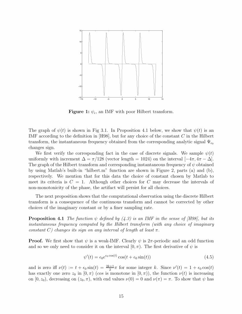
Figure 1: ψε, an IMF with poor Hilbert transform.

The graph of ψ(t) is shown in Fig 3.1. In Proposition 4.1 below, we show that ψ(t) is anIMF according to the definition in [H98], but for any choice of the constant C in the Hilberttransform, the instantaneous frequency obtained from the corresponding analytic signal Ψε0

changes sign.We first verify the corresponding fact in the case of discrete signals. We sample ψ(t)

uniformly with increment ∆ = π/128 (vector length = 1024) on the interval [−4π, 4π − ∆].The graph of the Hilbert transform and corresponding instantaneous frequency of ψ obtainedby using Matlab’s built-in “hilbert.m” function are shown in Figure 2, parts (a) and (b),respectively. We mention that for this data the choice of constant chosen by Matlab tomeet its criteria is C = 1. Although other choices for C may decrease the intervals ofnon-monotonicity of the phase, the artifact will persist for all choices.

The next proposition shows that the computational observation using the discrete Hilberttransform is a consequence of the continuous transform and cannot be corrected by otherchoices of the imaginary constant or by a finer sampling rate.

Proposition 4.1 The function ψ defined by (4.3) is an IMF in the sense of [H98], but itsinstantaneous frequency computed by the Hilbert transform (with any choice of imaginaryconstant C) changes its sign on any interval of length at least π.

Proof. We first show that ψ is a weak-IMF. Clearly ψ is 2π-periodic and an odd functionand so we only need to consider it on the interval [0, π). The first derivative of ψ is

ψ′(t) = ε0eε0 cos(t) cos(t + ε0 sin(t)) (4.5)

and is zero iff ν(t) := t + ε0 sin(t) = 2k+12

π for some integer k. Since ν ′(t) = 1 + ε0 cos(t)has exactly one zero z0 in [0, π) (cos is monotone in [0, π)), the function ν(t) is increasingon [0, z0), decreasing on (z0, π), with end values ν(0) = 0 and ν(π) = π. To show that ψ has

15

−15 −10 −5 0 5 10 15−20

−15

−10

−5

0

5

10

−15 −10 −5 0 5 10 15−0.5

0

0.5

1

1.5

2

2.5

3

3.5

a. b.

Figure 2: the Hilbert method for ψε: a. Imaginary part of discrete analytic sig-nal; b. Instantaneous frequency.

only one extremum on [0, π), it suffices to show that

ν(z0) <3

2π (4.6)

since then the only extremum of ψ on [0, π) will be the point eM where ν(eM) = π2. At the

point z0 we have cos(z0) = −1/ε0, which implies both π/2 < z0 < π and

sin(z0) =√

1 − (1/ε0)2.

Hence from the definition of ν it follows that

ν(z0) = z0 +√

ε20 − 1.

This implies that the condition (4.6) is equivalent to z0 < 32π−

√ε20 − 1. But cos is negative

and decreasing on [π/2, π], so we see that the desired relationship (4.6) just means thatcos(z0) > cos(3

2π−√ε2

0 − 1) should hold. The numerical value of the expression on the rightis smaller than −0.3382, while cos(z0) = −1/ε0 > −0.3368, hence the condition (4.6) holdsand ψ has exactly one local extremum in [0, π). Finally, since ε0 < π, the only zeros of ψ areclearly at the endpoints 0 and π, which verifies that ψ is an weak-IMF.

To see that ψ is in fact an IMF, we need to verify the condition on the upper and lowerenvelopes. Recall that it is 2π periodic and odd, therefore it has exactly one minimum in theinterval [−π, 0]. The cubic spline fit of the maxima (upper envelope) will be the constantfunction identically equal to 1. Similarly the cubic spline interpolant of the minima (lowerenvelope) will have constant value −1. This persists even for sufficiently large intervals ifone wishes to take finitely supported functions. Hence the function ψ satisfies the envelopecondition for an IMF from [H98]. We note that the general proof to show that for each 0 <

16

ε < ε, ψε is an IMF follows in a similar manner, where ε is the solution to the transcendentalequation 1/ε = sin(

√ε2 − 1) which arises in the limiting cases above. We observe that

ε ≈ 2.9716.Next we prove that for any selection of constant C, the corresponding instantaneous

frequency θ′C for ψ which is derived from an analytic method through (4.1) will have nontrivialsign changes. The denominator in formula (4.1) is always positive so it will suffice to provethat the numerator of θ′C changes sign for any choice of C. Using (4.3), (4.5) and the formula

Hψ′(t) = ε0 eε0 cos(t) sin(t + ε0 sin(t))

we can simplify the numerator of θ′C to the expression

ε0 eε0 cos(t)(eε0 cos(t) cos(t) − C cos(t + ε0 sin(t))

),

and so the sign of the term inside the parentheses

Nt(C) := eε0 cos(t) cos(t) − C cos(t + ε0 sin(t))

determines the sign of θ′C(t) at each point t ∈ [0, π). First observe that Nt(C) is a linearfunction of C for fixed t. For each value of C there is a point in [0, π) at which θ′C is negative,in fact N1.9(C) < −0.04 for C < 40 while N0.1(C) < −8 for C > 30. Similarly for any valueof C there is a point at which θ′C is positive since N0.1(C) > 4 for C < 13 and N1(C) > 2for C > 0. By continuity we see that for each value of the constant C the instantaneousfrequency θ′C obtained via the Hilbert transform is positive and negative on sets of positivemeasure. �

Finally, we mention that the L2 bandwidth of the analytic signal Ψ corresponding to asignal ψ also depends on the choice of the imaginary constant C. If Ψ is written in polarcoordinates as Ψ(t) = r(t)eiθ(t), the average frequency 〈ω〉 and the bandwidth ν2 have beendefined in [C95] as the quantities

〈ω〉 =

∫ω|S(ω)|2‖S‖2

2

dω =

∫θ′(t)

r2(t)

‖r‖22

dt, (4.7)

ν2 :=1

〈ω〉2∫

(ω − 〈ω〉)2 |S(ω)|2‖S‖2

2

dω (4.8)

=1

〈ω〉2∫ ((

r′(t)r(t)

)2

+ (θ′(t) − 〈ω〉)2

)r2(t)

‖r‖22

dt

=1

〈ω〉2∫ ((

r′(t)r(t)

)2

+ (θ′(t))2

)r(t)2

‖r‖22

dt − 1,

where S(ω) is the spectrum (Fourier transform) of ψ(t). The second equation in the dis-played sequence (4.8) follows immediately from Plancherel’s theorem along with standardproperties of the Fourier transform. If one chooses the constant C in the Hilbert transformso that ‖ψ‖2 = ‖Hψ‖2, then the computed bandwidth is ν2 = 0.1933 with mean frequency

17

< ω >= 2.7301. The discrete Hilbert transform computed by matlab for the sampled ψ hasthe same L2 bandwidth and mean frequency.

Summarizing, we observe that the example ψ given in (4.4) is a function which is

(i) an IMF in the sense of [H98];(ii) a monocomponent in the sense of [C95], i.e. its L2 bandwidth is small;(iii) “visually nice”,

but the analytic method fails to produce a monotone phase function.

Remark 4.1 The example considered in Proposition 4.1 also shows that adding the require-ment that the Hilbert transform (with a choice of the additive constant C = 3) of an IMFmust also be a weak-IMF, will not be sufficient to guarantee monotone phase.

A possible natural refinement of the definition of an IMF that would exclude these func-tions from the class of IMFs would be to require in addition that the first derivative of anIMF also be an IMF, or at least that the number of the inflection points equals the numberof extrema to within a count of one (i.e. a weak-IMF). The next example of a dampedsinusoidal signal (i.e. an amplitude modulated signal) shows that restrictions along theselines will not be able to avoid the same problem with instantaneous frequencies. We notethat this particular signal ψ is considered in [H98], but for the range of t from 1-512 sec.Since the function is not continuous periodic over this range, the expected Gibb’s effect atthe points t = 1 and 512 appears in that example, but is absent here.

Example 4.2 Let ψ(t) = exp(−0.01t) cos 232

πt, 8 ≤ t ≤ 520, then ψ is a continuous func-tion (of period 32) with a discontiniuty in the first derivative at t = 8. The signal ψ and allits derivatives are weak-IMFs. Both the conjugate operator and the computational Hilberttransform (applied to the sampled function with ∆t = 1) result in a sign changing instanta-neous frequency for any choice of the constant C. In Figure 3, we have provided a plot ofψ and the optimal instantaneous frequency (over all possible C) which is computed by theHilbert transform method. The values of both the continuous and computational results areto within machine precision at the plotted vertices.

In order to verify the properties of this example, we proceed as earlier in Example 4.1by first verifying the corresponding fact in the case of discrete signals. We sample ψ(t)uniformly with increment ∆ = 0.1 (vector length = 5121) on the interval [8, 520]. The graphof the Hilbert transform and corresponding instantaneous frequency of ψ obtained by usingMatlab’s built-in “hilbert” function are shown in Fig 3.3, parts (a) and (b), respectively.The next proposition shows that although other choices of the constant C may decrease theinterval where the instantaneous frequency is negative there is no value for C for which it isnonnegative on [8, 520]. Analogous to Example 4.1, it can be shown that the instantaneousfrequency changes its sign for any choice of the constant C.

Proposition 4.2 The function ψ in Example 4.2 and all its derivatives are weak-IMFson the interval [8, 512] whose instantaneous frequencies computed by the Hilbert transformmethod change sign for any choice of C.

18

0 100 200 300 400 500 600−1

−0.8

−0.6

−0.4

−0.2

0

0.2

0.4

0.6

0.8

0 100 200 300 400 500 600−0.8

−0.6

−0.4

−0.2

0

0.2

0.4

0.6

a. b.

Figure 3: Graphs for Example 4.2: (a) the IMF; (b) its instantaneous frequency.

Proof. To simplify the notation, we denote by ψ the function in Example 4.2 and use ψto denote ψ under the required linear change of variable from [8, 520] to [−π, π] in order toapply the continuous Hilbert transforms to the periodic function. In this case, ψ will be ofthe form

ψ(τ) = c exp(ατ) sin(kτ)

where k = 16. Next note that the derivatives of ψ are all of a similar form: ψ(n)(t) =c1e

αt cos(kt + c2). In particular, each derivative is just a constant multiple of ψ with aconstant shift of phase and hence are weak-IMF’s for any n = 0, 1, . . . ,∞. From formula (4.1)

applied at the zeros of ψ we have θ′C(zj) = − ψ′(zj)

Hψ(zj)+C, where the Hilbert transform is defined

through the conjugate operator (see [Z, K]) represented as a principal value, singular integraloperator

Hψ(zj) =1

πp.v.

∫ π

−π

ψ(t) cot(zj − t

2) dt. (4.9)

The standard identity

sin(kt) cot(t

2) = (1 + cos(kt)) + 2

k−1∑�=1

cos(�t) (4.10)

from classical Fourier analysis permits us to evaluate this expression by

Hψ(zj) =1

π

∫ π

−π

eαtT (t) dt, (4.11)

where T is an even trigonometric polynomial of degree 16 with coefficients depending onthe zj . Hence the values of Hψ at the zeros of ψ can be evaluated exactly (with Maple forexample). For z1 := 7

8π and z2 := 15

16π, the corresponding values of the Hilbert transform may

be estimated by Hψ(z1) ≤ 0.051 and Hψ(z2) ≥ 0.073 which verifies that Hψ(z2) > Hψ(z1).

19

On the other hand, ψ′(z1) = −keαz1 < 0 and ψ′(z2) = keαz2 > 0, therefore θ′(z1) =

− ψ′(z1)Hψ(z1)+C

is negative for C < −Hψ(z1) ≤ −0.051 and θ′(z2) = − ψ′(z2)Hψ(z2)+C

is negative for

C > −Hψ(z2) ≥ −0.073. From the fact that −Hψ(z2) < −Hψ(z1) we conclude that for anyC the instantaneous frequency is negative for at least one of the points z1 or z2. Finally, forthe extrema of ψ, say t = ξ we have θ′(ξ) = cHψ′(ξ)ψ(ξ), where c is a positive constant forany choice of C and it is easy to verify that there exists a value ξ such that Hψ′(ξ)ψ(ξ) > 0.Hence θ′(ξ) > 0 for any choice of C. �

We observe that, under the relaxed condition allowing the difference between the upperand lower envelopes to be within a given tolerance, ψ and its derivatives up to some finiteorder are (strong) IMF’s and the computational Hilbert transform method produces a nar-row bandwidth approximately equal to 0.0625.

The next result provides general information about the behavior of the instantaneousfrequency θ′ from any polar representation of ψ(t) = r(t) sin θ(t) in terms of a relationbetween the amplitude r and ψ.

Lemma 4.1 Suppose that ψ is a weak-IMF, r(t) > 0 is an amplitude such that ψ(t) =r(t) cos θ(t). Further, suppose that at some point t = τ , |ψ(τ)| �= r(τ) and ψ(τ) �= 0. Anecessary and sufficient condition for θ′(τ) to vanish is that

ψ′(τ)

ψ(τ)=

r′(τ)

r(τ), (4.12)

that is, that the logarithmic derivative of ψr

should vanish at t = τ .

Proof. Since r > 0 we can differentiate the relation cos θ = ψr

and get

−θ′ sin(θ) =ψ′r − r′ψ

r2=

ψ

r

(ψ′

ψ− r′

r

). (4.13)

To prove necessity, suppose that θ′(τ) = 0. Then since ψ(τ) �= 0, it follows from the identity

(4.13), that ψ′(τ)ψ(τ)

= r′(τ)r(τ)

.

To prove sufficiency it is enough to notice that in the event the left-hand side of (4.13)vanishes at t = τ , but θ′(τ) �= 0, then sin θ(τ) must vanish. Hence | cos θ(τ)| = 1 or|ψ(τ)| = r(t), which is a contradiction. Hence θ′(τ) = 0. �

Looking back, one can see that Lemma 4.1 can be used to motivate the proof of the char-acterization theorem for weak-IMF’s (Theorem 3.1). Indeed, for the envelopes constructedthere, r′

rand ψ′

ψwere forced to have different signs and therefore they can not be equal at

any point that is not a zero of ψ. From Lemma 4.1, it follows that θ′ does not change signbetween any two zeros of ψ. Since θ′ is continuous and was forced to be nonzero at the zerosof ψ, we have that θ′ cannot change sign.

Proposition 4.3 Let va(t) be an even function defined on (−π, π] such that va(0) = 0 andeva/‖eva‖L1 → δ, where δ is the Dirac delta function. Define ψa(t) := eva(t) cos(kt). Then

20

there exists a value of a0 sufficiently large such that the analytic instantaneous frequency forψa for any a > a0 changes sign for any choice of the constant used in defining the Hilberttransform Hψa.

Proof: Recall from (4.9) that a Hilbert transform of ψa at a point t ∈ (−π, π] is Hψa(t)+C,where C is an arbitrary real constant and

Hψa(t) = p.v.1

π

∫ π

−π

ψa(τ) cott − τ

2dτ (4.14)

is the conjugate operator for periodic functions. Using two applications of the identity (4.1),we observe that the analytic method produces an instantaneous frequency of the form

θ′C =ψaHψ′

a − (Hψa + C)ψ′a

(Hψa + C)2 + ψ2a

= Rθ′0 − C Lψ′a, (4.15)

where R and L are positive functions on (−π, π]. Let zj = 2j−12k

π, −k + 1 ≤ j ≤ k be thezeros of ψa, then

sgn(ψ′a(zj)) = (−1)j (4.16)

and by (4.15), with C = 0, it follows that

θ′0(zj) = − ψ′a(zj)

Hψa(zj)(4.17)

and consequentlysgn(θ′0(zj)) = (−1)j+1sgn(Hψa(zj)). (4.18)

The proof of the lemma will be completed if we can show that for sufficiently large athere is an index J for which two consecutive values of Hψa(zj) have the same sign

sgn (Hψa(zJ)) = sgn (Hψa(zJ+1)) =: σ. (4.19)

When C = 0 this follows immediately from equation (4.18). For C �= 0, we use the analogueof (4.18),

sgn(θ′C) = −sgn(ψ′a) sgn(Hψa + C) (4.20)

which follows immediately from (4.15). In the case sgn(C) = σ, this last identity showsthat θ′C has different signs at the endpoints of (zJ , zJ+1), since ψ′

a does. For the final case,sgn(C) = −σ, we observe that Hψa and ψ′

a are both odd functions since ψa is even. Byconsidering −zJ and −zJ+1 in place of zJ and zJ+1, we see that sgnH(ψa) = −σ = sgn(C) atthese two points and so once again from (4.20), θ′C has different signs at the endpoints. Henceby the continuity of θ′C , there are nonempty intervals where the instantaneous frequency takeson opposite sign.

Therefore to complete the proof, we must verify (4.19), i.e., for parameter a > 0 suffi-ciently large, there is a pair of consecutive points zJ , zJ+1, such that H(ψa) does not change

21

sign. Evaluating the conjugate operator at the zeros x = zj in (4.9), we can proceed as inProposition 4.2 using the periodicity of ψa and the trigonometric identity (4.10), to obtain

Hψa(zj) = c

∫ π

−π

eva(t) cos(kt) cotzj − t

2dt

= c

∫ π

−π

eva(t+zj) sin(kt) cott

2dt

= c

∫ π

−π

eva(t+zj)Pk(t) dt,

where in the last identity Pk(t) is a trigonometric polynomial of degree k. Therefore it followsthat

lima→∞

Hψa(zj)

‖eva‖ = Pk(0) = − cotzj

2.

holds. For any zm, zm+1 ∈ (0, π) it is follows easily that there exists a > 0 such thatsgn(Hψa(zm)) = sgn(Hψa(zm+1)). Hence for a is sufficiently large, ψa is a weak-IMF. �

We note that the arguments in Proposition 4.3 can also be used to explain the behaviorof θ′ in Example 4.2.

Example 4.3 We illustrate in Figure 4 the use of Proposition 4.3 in producing additionalweak-IMF’s with non-monotone phase. For the sample function ψ, we set k = 16 and let va

be a gaussian with standard deviation s = .01 and centered at the origin. The perturbationis applied at both t1 = 0 and t2 = π/32. The function ψ is displayed in part (a), its hilberttransform in part (b), and its instantaneous frequency in part (c).

For this same function, in Figure 4(d) we illustrate the application of Lemma 4.1. Theinstantaneous frequency changes sign when the logarithmic derivative of ψ

rvanishes at points

other than at an acceptable zero: either a zero of (i) ψ or of (ii) its Hilbert transform, i.e.points where |f | = r. Notice that the endpoints of the two intervals where the instantaneousfrequency becomes negative corresponds precisely to the four (non-acceptable) zeros of thelogarithmic derivative of ψ/r

Example 4.4 An informative example of function which may be considered a true IMF isgiven by the function

ψ(t) = (t2 + 2) cos(π sin(8t))/16, − 4π ≤ t ≤ 4π (4.21)

which, along with its instantaneous frequency, is plotted in Figure 5. Notice that t2 + 2 maybe regarded as an envelope of ψ and that it is close but different than the upper envelopeproduced by a cubic spline fit through the maxima. Recall from the observation in Section 2.1that a necessary and sufficient for the IMF envelope condition (b) of Definiton 2.1 to besatisfied is that those envelopes reduce to a quadratic polynomial. This example shows thatthe sifting convergence criterium in the EMD process for measuring the difference of theabsolute values of the upper and lower envelopes should be chosen with care. If fact, it can be

22

4 (a):

−10 −5 0 5 10

−2.5

−2

−1.5

−1

−0.5

0

0.5

1

1.5

2

2.5

4 (b):

−0.6 −0.4 −0.2 0 0.2 0.4 0.6−1.5

−1

−0.5

0

0.5

1

1.5

4 (c):

−0.6 −0.4 −0.2 0 0.2 0.4 0.6−20

0

20

40

60

80

100

4 (d):

−0.6 −0.4 −0.2 0 0.2 0.4 0.6−40

−30

−20

−10

0

10

20

30

40

Figure 4: Sample IMF from Example 4.3: a. Cosine signal with strong pertur-bation at 0 and π/16; b. the Hilbert tranform of ψ near the pertur-bations; c. the instantaneous frequency of ψ near the perturbations;d. the logarithmic derivative of ψ/r near the perturbations.

23

−15 −10 −5 0 5 10 15−10

−8

−6

−4

−2

0

2

4

6

8

10

−15 −10 −5 0 5 10 15−800

−600

−400

−200

0

200

400

a. b.

Figure 5: Plot of the example IMF defined by equation (4.21): a. The IMF ψwith a parabolic envelope, b. Instantaneous frequency.

easily verified that smoothing off the endpoint data of this example will result in a functionfor which the EMD residual can be made visually negligible after a single sifting. There aremany variations of these examples to produce similar behavior.

We conclude this section with a procedure that adds a smooth disturbance at an ap-propriate scale to any reasonable function in such a way that the function maintains itssmoothness and analytical profile, that is, no additional extrema are introduced and theexisting extrema are only perturbed, but the resulting function has non-monotone analyticphase. By a reasonable function ψ, we will mean an IMF in the strongest sense, which wecall a Hilbert-IMF.

Definition 4.1 A function is called a Hilbert-IMF if it satisfies the following conditions:(i.) ψ is an IMF in the sense of the definition in [H98];(ii.) the analytic signal of ψ (i.e. via the Hilbert transform) Ψ = reiθ, r′ and θ′ are

smooth functions and θ′ > 0;(iii.) the weighted L2 bandwidth is small.

The idea of the perturbation procedure is based on the fact that by multiplying theanalytic function Ψ = reiθ by another analytic function, say Γ = r1e

iθ1 , the result ΨΓ =rr1e

i(θ+θ1) is also analytic with analytic amplitude rr1 and analytic phase θ + θ1. Since θ′

and θ′1 are smooth functions, in order to force the instantaneous frequency of ΨΓ to changesign it suffices to choose Γ such that θ′1(T ) < −θ′(T ) at some point T . One way we caninsure that the weighted L2 bandwidth of ΨΓ remains small is to localize the perturbation Γto a small interval I, i.e. both r1 and θ1 should decay rapidly to zero outside I. Further, toguarantee that the real part of ΨΓ is an IMF in the sense of [H98], the added perturbationmust only result in a small deviation of the zeros and extrema of the original IMF Ψ, and

24

should not introduce additional zeros nor extrema. This is achieved by incorporating anadditional tuning parameter σ into our perturbation Γσ, for small values of σ.

The technique used in the proof of the results below shows that there are many functionsthat can be used as such perturbation functions. We consider one particular smooth functionthat is constructed from the modified Poisson kernel

yρ(t) :=(1 − ρ)2

1 − 2ρ cos t + ρ2, 0 ≤ ρ < 1. (4.22)

It is well known that its conjugate function is Hyρ(t) = 1−ρ1+ρ

2ρ sin t1−2ρ cos t+ρ2 . Although it is an

abuse of notation, we will refer to these simply as y and Hy with the understanding thatthe parameter ρ is implicitly present. We define the perturbation Γ in terms of y = yρ by

Γ = Γρ := exp(−Hy + iy). (4.23)

and observe that as the parameter ρ approaches 1 from below, the function Γρ becomes verylocalized.

The perturbed IMF is set to �(ΨΓσ) = re−σHy cos(θ + σy) for some real σ. The idea inbrief is to select σ small and ρ sufficiently close to 1 so that the change in the functional valuesare also small, i.e., the zeros, extrema, and the extremal values are perturbed slightly fromthe original IMF. On the other hand, the corresponding instantaneous frequency becomesθ′ + σy′ (see Lemma 4.2 below). Moreover, y′ has one local minimum that is negative withmagnitude depending on ρ. In the special case when r = eAt and θ = mt on an interval (thelength of the interval can be arbitrarily small), we prove in Corollary 4.2 that there existsa subinterval and values of the parameters σ and ρ such that under mild conditions, theperturbed function satisfies all the properties i-iii), but has non-monotone phase. From theproof and by continuity it is then clear that the new instantaneous frequency can be madenegative on an interval while preserving all other properties listed in i-iii). A similar resultholding for more general functions is established in Corollary 4.3.

To show that the perturbed function is a weak-IMF we utilize the logarithmic derivativeas ρ → 1− and the following technical Lemma, where we establish that the maximum ofHy′ and its value at the minimum of y′ behave asymptotically as a finite multiple of theminimum value of y′.

Lemma 4.2 Let 0 ≤ ρ < 1 and y = yρ be defined as in equation (4.22), then the followingproperties hold:

(a) for all σ > 0 the function Γσ defined in equation (4.23) is analytic with amplitudee−σ Hy and phase σ y;

(b) if −µ := min y′ = y′(t0), then limρ→1−

Hy′(t0)µ

=1√3.

(c) limρ→1−

µ

max |Hy′| =3√

3

8.

(d) The function Hy′ is even with exactly one positive zero, tz which satisfies 0 < t0 < tz

and limρ→1−

y′(tz)µ

= 0.

25

Proof. Part (a) follows from the construction of the analytic function Γ and the fact that|Γ| > 0. To establish part (b) we determine the minimizer of y′, which we denote t0, fromthe equation y′′(t0) = 0, which is equivalent to the equation

2ρ cos2 t0 + (1 + ρ2) cos t0 − 4ρ = 0. (4.24)

Hence there exists a unique solution t0 which satisfies the relation cos t0 = D−(1+ρ2)4ρ

, where

D :=√

ρ4 + 34ρ2 + 1. Substituting this explicit formula for cos t0 into the expression fory′(t0), the minimum value of y′ can be written as

y′(t0) = −2(1 − ρ)2

√2(1 + ρ2)D − (2ρ4 + 20ρ2 + 2)

(3ρ2 + 3 − D)2. (4.25)

Proceeding similarly with the expression for Hy′(t) given by

Hy′(t) = −2ρ(1 − ρ)

1 + ρ

(1 + ρ2) cos t − 2ρ

(1 − 2ρ cos t + ρ2)2(4.26)

we find, after algebraic rationalization and simplification, that

Hy′(t0)µ

=2√

2 ρ√(1 + ρ2)D + ρ4 + 10ρ2 + 1

. (4.27)

Part (b) follows immediately by taking the limit as ρ → 1−.Part (c) is established in a similar manner by observing from equation (4.26) that

max |Hy′| = Hy′(0) = 2ρ1−ρ2 and so, using the identity (4.25), it follows that µ

Hy′(0) con-

verges to 3√

38

as ρ → 1−.Finally, for part (d) we determine from (4.26) that zeros of Hy′ are exactly the roots of

the equation cos t = 2ρ1+ρ2 . Substituting this expression for cos tz into the left-handside of

the equation (4.24) for cos t0, we get a negative value −2ρ(1−ρ2)2

(1+ρ2)2for the quadratic expression

and so cos tz < cos t0, which is equivalent to t0 < tz. Observing that sin tz = 1−ρ2

1+ρ2 , we can

use this identity to evaluate y′(tz) to obtain y′(tz)µ

= −2ρ(1−ρ)(1+ρ)µ

→ 0 as ρ → 1−. �

In Corollary 4.2 we prove in the special case r = eAt, A ≤ 0 and θ = mt that we canfind values of σ and ρ such that the procedure described above produces a desired functionsatisfying the properties i-iii) but whose analytic instantaneous frequency changes sign. Wefirst prove a milder version in the following proposition, and then modify the parameter σto establish the stronger version.

Proposition 4.4 Let the notation be as in the previous lemma (Lemma 4.2). In particular,let t0 be the point which provides a global minimum for y′, tz be the positive zero of Hy′

and µ := −y′(t0). Suppose further that A ≤ 0. If ψ(t) := exp(At) cos mt, then there exist aconstant ρ∗ and a point t∗ such that for ρ∗ < ρ < 1

ψ(t) = exp(At − m

µHy(t− t∗)) cos(mt +

m

µy(t − t∗)), (4.28)

26

is a weak-IMF, but its analytic instantaneous frequency vanishes at t0 + t∗. Moreover, thedifference between absolute values of the upper and lower cubic spline envelopes is smallexcept at the endpoints in the case that A is negative.

Proof. From the previous discussion and from the representation ψ(t) = �(Ψ(t)Γmµ (t− t∗))

it is clear that the analytic phase of ψ is θ = mt + mµy(t − t∗). The definition of µ implies

that the expression m + mµy′(t − t∗) is nonnegative and vanishes only at the point t0 + t∗,

hence θ is strictly increasing. Furthermore, we show that if ρ is close to 1, the rapid decayof y(t − t∗) away from t0 + t∗ will insure that the zeros of ψ and ψ are the same in numberand are separated only slightly from one another.

We may assume that the perturbation y = yρ is added between a maximum of ψ and thezero τ0 immediately following; the other three situations can be handled in the same waywith an appropriate changes of the signs of the corresponding expressions. Denote by τ− thenearest point less than τ0 which satisfies tanmτ− = 32

3√

3. Any point from the interval (τ−, τ0)

can be picked for t∗. We select t∗ := τ0+τ−2

, δ := τ0−τ−4

and set ∆ := (t∗ − δ, t∗ + δ). Byconstruction it is clear that functions y, Hy, y′, and Hy′ (translated by t∗) tend uniformly tozero outside the interval ∆ as ρ approaches 1−. Hence ψ uniformly tends to ψ outside ∆.

Since ψ and ψ′ have only simple zeros, it follows that there exists ρ1 such that for any1 > ρ > ρ1 the perturbed function ψ is a weak-IMF; even more, for each zero and extrema

of ψ there corresponds exactly one zero and extrema of ψ. To prove this, we consider the

functions on three disjoint sets, a subinterval ∆∗ of ∆ (to be determined), the set ∆\∆∗,and the complement of ∆.

We first consider the set of values t in the complement of ∆. Assume that there is asequence of ρ′s approaching 1 from below so that there is an extrema of ψ, say τe, such thatin a neighborhood of that extrema ψ has at least three extrema (the extrema must be odd in

number since ψ tends uniformly to ψ). By Rolle’s theorem and the uniform convergence as

ρ → 1−, it follows that ψ′ has a multiple zero at τe, which is a contradiction. Hence outside∆, ψ is an IMF.

Consider now the interval ∆. To follow the changes of the extrema of ψ, we consider the

logarithmic derivative of ψ given by

L :=ψ′

ψ= A +

m

µ(−Hy′(t − t∗)) − (m +

m

µy′(t − t∗)) tan(mt +

m

µy(t − t∗)).

We show L is negative on ∆. It then follows that ψ has no additional extrema on this

interval, and so ψ will be an IMF in the sense of the definition in [H98], but its analyticinstantaneous frequency m + m

µy′ has a zero.

To see that L is negative on ∆, observe that for a fixed ρ (1 > ρ > ρ1) since A ≤ 0,tan(mt + m

µy(t − t∗)) > 0, and (m + m

µy′(t − t∗)) ≥ 0 it follows that L < 0 on the interval

∆∗ := (t∗ − tz, t∗ + tz), where tz is specified in part (d) of Lemma 4.2. From the proof

of that Lemma, we see that tz approaches 0 as ρ approaches 1− and hence we can pick ρ2

(1 > ρ2 > ρ1) such that ∆∗ ⊂ ∆ for each ρ for which 1 > ρ ≥ ρ2.

27

On the other hand, for any t outside ∆∗, we have that m + mµy′(t) > m + m

µy′(tz)

and from Lemma 4.2(d) it follows that there exists 1 > ρ3 > ρ2 such that the inequalitym + m

µy′(t) > m

2holds for any 1 > ρ > ρ3 and any t ∈ ∆\∆∗. Finally from Lemma 4.2,

we can pick 1 > ρ∗ > ρ3 such that the inequality max |Hy′|µ

< 163√

3holds for any ρ > ρ∗. The

choice of the point t∗ and the fact that y is a positive function provide the inequality

tan(mt +m

µy(t− t∗)) > tan(mτ−) =

32

3√

3

for any t ∈ ∆\∆∗. Using the above estimates and the assumption A ≤ 0 we have that

L < mmax |Hy′|

µ− m

2tan(mt +

m

µy(t− t∗)) < 0,

for any t ∈ ∆\∆∗ and any 1 > ρ > ρ∗, which completes the proof. �

Corollary 4.2 Let ψ be the Hilbert-IMF considered in Proposition 4.4. Then there existσ > m

−µsuch that the small perturbation of ψ, ψ = �(ΨΓσ), satisfies parts (i) and (iii) of

the definition of a Hilbert-IMF, but has does not have monotone analytic phase.

Proof. Since ψ and all other related functions considered in Proposition 4.4 depend contin-

uously on σ, and for σ = −mµ

we have that θ′ vanishes only at the point t0 + t∗, it followsthat any increase of σ forces the instantaneous frequency to be negative in a neighborhoodof that point. On the other hand, by the choice of ρ∗( 1 > ρ∗ > 0) from Proposition 4.4and the uniform convergence, it follows that there exists σ∗ > −m

µsuch that the perturbed

function ψ is a weak-IMF outside ∆ and Lσ∗ is negative on ∆; i.e. there are no additional

zeros and extrema on ∆. Hence ψ is a nicely behaved function with analytic instantaneousfrequency that changes sign on an interval of positive measure. �

Remark 4.2 The condition A ≤ 0 can be relaxed to A < m√3

which agrees with the estimate

in Lemma 4.2(b). The proof of the Proposition 4.4 with that restrictiion requires furthertechnical estimates as in Lemma 4.2(d) for a point tη such that 0 < t0 < tη and

limρ→1−

y′(tη)µ

= η − 1

for a fixed 0 < η < 1. Details of the estimates are similar so we do not include them here.

Example 4.5 To illustrate the above construction, we consider the function Ψ = e4it, −π <t ≤ π, and apply the procedure twice for ρ = 0.95 and σ = 0.31, once at the point t1 = −2.1and again at the point 0.2. The resulting signal and its analytic instantaneous frequency areshown on Figure 6.

For any nice function (e.g. a Hilbert-IMF) ψ = r cos θ with only simple zeros, it is clearfrom the identity ψ′

ψ= r′

r− tan θ θ′ that if there exist a zero for which r′ �= 0 then the

logarithmic derivative ψ′ψ

and the instantaneous bandwidth r′r

have the same sign in a one-sided neighborhood of that zero. Then if the perturbation is added in that neighborhood,

28

−4 −3 −2 −1 0 1 2 3 4−1

−0.8

−0.6

−0.4

−0.2

0

0.2

0.4

0.6

0.8

1

−4 −3 −2 −1 0 1 2 3 4−1

0

1

2

3

4

5

6

7

a. b.

Figure 6: Plot of the IMF in Example (4.5): a. an IMF perturbed by a smoothperturbation; b. Instantaneous frequency.

the proof of Proposition 4.4, without significant modifications, can be used to prove similarresults so long as r′

r+ 9

8√

3maxI θ′ is negative in a neighborhood of that zero, as established

in the next Corollary. We note that by choosing ρ closer to 1, the interval I can be madearbitrarily small.

Corollary 4.3 Let ψ = r cos θ be the restriction to the circle of any function analytic in adisk of radius larger than one. Assume that ψ is an IMF in the sense of [H98] with amplituder and monotone phase θ which are defined using the Hilbert transform. Suppose further thatψ has only simple zeros, that there exists a zero z0 of ψ for which r′

rand ψ′

ψhave the same

sign in a one-sided neighborhood I of z0, and that r′r

+ 98√

3maxI θ′ < 0 on I, then there exist

parameters ρ∗ and σ∗, and a point t∗ such that the function ψ(t) = �(Ψ(t)Γσ∗(t− t∗)) is an

IMF with zeros and extrema which are close perturbations of those of ψ, but with an analytic

instantaneous frequency θ′(t) = θ′ + σy′(t − t∗) which changes sign.

Proof. As in Proposition 4.4, it is enough to prove that θ′(T ) = 0 for some point T . Wemay assume from the hypothesis that θ′ > 0, then the modified instantaneous frequencyθ(t) = θ′(t) + σy′(t− t∗) > 0 for small σ. Hence if σ is continuously increased, by continuitywe will reach a value σ1 for which θ′(T ) = 0 for some point T and is positive elsewhere. If ρis then increased close to 1, and σ1 is adjusted accordingly, we can localize the perturbationon an arbitrarily small interval with θ′ vanishing at a point.

Notice that the instantaneous bandwidth does not change sign on an interval that containsboth I and z0 as an interior point. We may assume that L < 0 on I, then the logarithmicderivative of ψ is

L(t) =r′(t)r(t)

− σHy′(t − t∗) − θ′(t) tan θ(t).

29

From the choice of σ it follows that maxI θ′ − σµ ≥ 0 and hence σ ≤ maxI θ′µ

. For the new

instantaneous bandwidth as ρ → 1−, we have r′r−σHy′(t− t∗) ≤ r′

r+maxI θ′ max|Hy′|

µ→ r′

r+

98√

3maxI θ′ < 0 on I, where the last inequality is the assumption on ψ relating instantaneous

bandwidth and frequency. Since I is a finite interval, there exists ρ∗ such that L < 0 for anyρ satisfying 1 > ρ > ρ∗. On the other hand, since θ′ ≥ 0 and tan θ > 0 on I it follows thatL < 0 on I. All other steps are the same as in the proof of Proposition 4.4. �

Remark 4.3 The condition on the logarithmic derivatives (of the function ψ and its am-plitude r) to have the same sign in a neighborhood of a zero is equivalent to r′(z0) �= 0, orr′(z0) = 0 but r′ψ′ψ > 0 on I. In other words if all other requirements are met, the procedureworks more generally than in the case of envelopes considered in the Theorem 3.1.

Remark 4.4 The procedure for adding perturbations to a nice function can be also used forremoving certain types of noise. If a function has a negative instantaneous frequency onsome small interval, then we can apply the procedure with a perturbation Γσ using negative σin order to remove negative instantaneous frequencies, but still preserve the general features(zeros, local extrema) and smoothness class of the original function.

References

[BS] C. Bennett and R. Sharpley, Interpolation of Operators, Academic Press, New York,1988.

[BR] G. Birkhoff and G.C. Rota, Differential Equations, (4-th ed) Wiley, New York, NY,1989.

[C95] L. Cohen, Time-Frequency Analysis, Prentice-Hall Signal Processing Series, UpperSaddle River, NJ, 1995.

[H98] N.E. Huang, Z. Shen, S.R. Long, M.C. Wu, H.H. Shih, Q. Zheng, N.C. Yen, C.C.Tung, and H.H. Liu, The empirical mode decomposition and the Hilbert spectrumfor nonlinear and non-stationary time series analysis, Proc. Royal Soc. Lond. A 454(1998), 903-995.

[H99] N.E. Huang, Z. Shen, and S.R. Long, A new view of nonlinear water waves: the Hilbertspectrum, Annu. Rev. Fluid Mech. 31 (1999), 417–457.

[K] Y. Katznelson, An Introduction to Harmonic Analysis, (2-nd ed.), Dover Pubns, 1976.

[M] S.L. Marple, Computing the discrete-time analytic signal via FFT, IEEE Transactionson Signal Processing 47 (1999), 2600-2603.

[P] M.A. Pinsky, Introduction to Fourier Analysis and Wavelets, Brooks/Cole, PacificGrove, 2002.

30

[S] E.M. Stein, Singular Integrals and Differentiability Properties of Functions, PrincetonUniversity Press, Princeton, 1970.

[V] V. Vatchev, Intrinsic Mode Functions and the Hilbert Transform, Ph.D Dissertation,Department of Mathematics, University of South Carolina, 2004.

[Z] A. Zygmund, Trigonometric Series, Cambridge University Press, Cambridge, 1969.

Industrial Mathematics InstituteDepartment of MathematicsUniversity of South CarolinaColumbia, SC 29208

E-mail: sharpley@math.sc.edu, vatchev@math.sc.edu

31