Submitted toJournal of the Mathematical Society of Japan

Upper bounds for the dimension of tori acting on GKM manifolds

By Shintaro Kuroki

Abstract. The aim of this paper is to give an upper bound for the dimension

of a torus T which acts on a GKM manifold M effectively. In order to do that, weintroduce a free abelian group of finite rank, denoted by A(Γ, α,∇), from an (abstract)(m,n)-type GKM graph (Γ, α,∇). Here, an (m,n)-type GKM graph is the GKM graphinduced from a 2m-dimensional GKM manifold M2m with an effective n-dimensional

torus Tn-action which preserves the almost complex structure, say (M2m, Tn). Then itis shown that A(Γ, α,∇) has rank ℓ(> n) if and only if there exists an (m, ℓ)-type GKMgraph (Γ, α,∇) which is an extension of (Γ, α,∇). Using this combinatorial necessaryand sufficient condition, we prove that the rank of A(ΓM , αM ,∇M ) for the GKM graph

(ΓM , αM ,∇M ) induced from (M2m, Tn) gives an upper bound for the dimension ofa torus which can act on M2m effectively. As one of the applications of this result,we compute the rank associated to A(Γ, α,∇) of the complex Grassmannian of 2-planesG2(Cn+2) with the natural effective Tn+1-action, and prove that this action on G2(Cn+2)

is the maximal effective torus action which preserves the standard complex structure.

1. Introduction

GKM manifolds (or more general spaces) are “roughly” spaces with torus action whose 0- and

1-dimensional orbits have the structure of a graph. This class of spaces first appeared in the work of

Goresky-Kottwitz-MacPherson [8] as a class of algebraic varieties (GKM stands for their initials).

Motivated by their work, Guillemin-Zara [11] introduce a combinatorial counterpart of the GKM

manifold, called a(n) (abstract) GKM graph, and give some relationships between the (symplectic)

geometry (and topology) of GKM manifolds and the combinatorics of GKM graphs. This leads

to the study of geometric and topological properties of the GKM manifolds using combinatorial

properties of GKM graphs (see e.g. [6, 7, 9, 10, 15, 17, 19, 20] etc). In this paper, we introduce

a new invariant of GKM graphs and provide a partial answer to the extension problem of torus

actions on GKM manifolds.

To state our main results more precisely, we briefly recall the setting of this paper and back-

ground of the extension problem of torus actions. Let Tn be the n-dimensional torus and M2m be

a 2m-dimensional, compact, connected, almost complex manifold with effective Tn-action, which

preserves the almost complex structure. We denote such a manifold by (M2m, Tn), or M2m, M ,

(M,T ) (if its torus action or dimensions of the manifold and torus are obviously known from the

context). We call (M2m, Tn) a GKM manifold if it satisfies the following properties (see Section 4

for details):

1. the set of fixed points is not empty and isolated, i.e., MT is 0-dimensional;

2. the closure of each connected component of 1-dimensional orbits is equivariantly diffeomor-

phic to the 2-dimensional sphere, called an invariant 2-sphere.

By regarding fixed points as vertices and invariant 2-spheres as edges, this condition is equivalent

to the one-skeleton of (M2m, Tn) having the structure of a graph, where the one-skeleton of

(M2m, Tn) is the orbit space of the set of 0- and 1-dimensional orbits. Note that there are

several definitions of GKM manifolds (see e.g. [9, 11] etc). This is because the spaces with such

torus actions have been studied from several different points of view (homotopically, topologically,

algebraically and geometrically). In this paper, we study the GKMmanifolds defined by Guillemin-

Zara in their original paper [11]. In particular, equivariant formality is often assumed for the

cohomology of GKM spaces. However, in this paper, we do not need to use this assumption;

therefore, our definition of a GKM manifold is more general than the equivariantly formal GKM

manifolds (see Section 4).

2010 Mathematics Subject Classification. Primary 57S25; Secondary 94C15.Key Words and Phrases. GKM graph, GKM manifold, Torus degree of symmetry.

2 S. Kuroki

For example, in our setting, the following manifolds are GKM manifolds: non-singular com-

plete toric varieties (also called toric manifolds) and homogeneous manifolds G/H (where G is a

compact connected Lie group and H is its closed subgroup with the same maximal torus) with

torus invariant almost complex structures such as S6 = G2/SU(3), flag manifolds and complex

Grassmannians, etc.

Since GKM manifolds are even-dimensional and their effective torus actions have isolated fixed

points, the differentiable slice theorem tells us that the following inequality holds for every GKM

manifold (M,T ):

dimT ≤ 1

2dimM.

If the equality dimT = 12 dimM holds, such a GKM manifold is also known as a torus manifold

(with invariant almost complex structure); famous examples are toric manifolds. Namely, by

definition, the torus action on a torus manifold is maximal, i.e., the torus action can not be

extended to a bigger torus action. In this case, the author, Masuda and Wiemeler [13, 14, 16, 22]

have studied the extended G-actions of T -actions on torus manifolds, where G is a non-abelian,

compact, simply connected Lie group with maximal torus T . On the other hand, for general GKM

manifolds, the given torus action might not be maximal. In fact, a restricted Tm−1-action of a 2m-

dimensional toric manifold (M2m, Tm) is often a GKM manifold (M2m, Tm−1), in other words,

this GKM manifold (M2m, Tm−1) extends to a toric manifold (M2m, Tm). Thus the following

problem naturally arises in the GKM manifolds (also see Proposition 4.3):

Problem 1.1. When does a GKM manifold (M2m, Tn) extend to a GKM manifold

(M2m, T ℓ)? Here, Tn ⊂ T ℓ and n < ℓ ≤ m.

As not every GKM manifold can be endowed with a torus T ℓ-action, that extends the given

action and makes it a torus manifold, in this paper we give a combinatorial method to determine

an upper bound for ℓ. Namely we first introduce a free abelian group with finite rank A(Γ, α,∇),

called a group of axial functions, for the GKM graph (Γ, α,∇) in Section 2. Here, a GKM graph

is “roughly” the following triple (see Section 2 for details): an m-valent graph Γ; a function

α : E(Γ) → H2(BTn) ≃ Zn, called an axial function; and a collection ∇ of some bijective maps

between out-going edges on adjacent vertices, called a connection. We call such a GKM graph an

(m,n)-type GKM graph in this paper. The main theorem of this paper can be stated as follows

(see Sections 2 and 3 for details):

Theorem 1.2. Let (Γ, α,∇) be an abstract (m,n)-type GKM graph. Then, the following two

statements are equivalent:

1. rk A(Γ, α,∇) ≥ ℓ for some n ≤ ℓ ≤ m;

2. there is an (m, ℓ)-type GKM graph (Γ, α,∇) which is an extension of (Γ, α,∇).

As a GKMmanifold (M2m, Tn) defines an (m,n)-type GKM graph (see Section 4), Theorem 1.2

implies that the maximal dimension of a torus which can act on a GKM manifold M is bounded

from above by the rank of the group of axial functions of the GKM graph induced from M .

Namely, we obtain the main result of this paper as follows (see Section 4 for details):

Corollary 1.3. Let (M2m, Tn) be a GKM manifold and (ΓM , αM ,∇M ) be its (m,n)-type

GKM graph. Assume that rk A(ΓM , αM ,∇M ) = ℓ. Then, the Tn-action on M2m does not extend

to any T ℓ+1-action preserving the given almost complex structure.

In particular, if rk A(ΓM , αM ,∇M ) = n, then the Tn-action on M2m is maximal among torus

actions which preserve the given almost complex structure.

Remark 1.4. Shunji Takuma also obtains a partial answer to Problem 1.1 by introducing

an obstruction class for the extension of an (m,n)-type GKM graph to an (m,n+ 1)-type GKM

graph in his note [19]. Theorem 1.2 may be regarded as the generalization of his result.

Upper bounds for the dimension of tori acting on GKM manifolds 3

Problem 1.1 is reminiscent of the computation of the torus degree of symmetry of a manifold

X (see [12]), i.e., the maximal dimension of a torus which can act on X effectively. A torus

degree of symmetry has been studied for many classes of manifolds, in particular from differential

geometry (see e.g. [4, 12, 21, 23]). Corollary 1.3 may be regarded as giving an upper bound of

the torus degree of symmetry of an invariant almost complex structure of a GKM manifold. As an

application of Corollary 1.3, in the final section (Section 5), we compute the torus degree of such

symmetry for the complex Grassmannian of 2-planes, denoted as

G2(Cn+2) ≃ GL(n+ 2,C)/GL(2,C)×GL(n,C) ≃ U(n+ 2)/U(2)× U(n).

Namely, we compute rk A(ΓM , αM ,∇M ) forM = G2(Cn+2) with the natural effective Tn+1-action

and prove the following fact:

Proposition 1.5. The standard effective Tn+1-action on G2(Cn+2) is maximal among the

effective torus actions which preserve the almost complex structure.

Note that there is the natural Tn+2-action on G2(Cn+2) which is induced from the maximal

torus subgroup in U(n+ 2). However, this action is not effective.

The organization of this paper is as follows. In Section 2, we recall an abstract GKM graph

(Γ, α,∇), and introduce its group of axial functions A(Γ, α,∇). In Section 3, the main theorem

(Theorem 1.2) is proved. In Section 4, in order to apply our results to geometry, we recall the

definition of a GKM graph induced from a GKM manifold, and prove Corollary 1.3. We also prove

the T 2-action on S6 = G2/SU(3) is maximal. In Section 5, we obtain the GKM graph obtained

from the effective Tn+1-action on G2(Cn+2), and compute its group of axial functions. This proves

Proposition 1.5.

2. GKM graph and its group of axial functions

In this section, we first recall the basic facts about GKM graphs (Γ, α,∇) (see [11]) and

introduce the extension of axial functions of GKM graphs precisely. Then a finite rank free

abelian group A(Γ, α,∇), called a group of axial functions, is defined.

2.1. GKM graph and its extension

We first prepare some notation to define a GKM graph. Let Γ = (V (Γ), E(Γ)) be an abstract

graph comprising of a set V (Γ) of vertices and a set E(Γ) of oriented edges. For a given orientation

on e ∈ E(Γ), we denote its initial vertex by i(e) and its terminal vertex by t(e). In this paper,

we assume that there are no loops in E(Γ), i.e., i(e) = t(e) for any e ∈ E(Γ), and Γ is connected.

The symbol e ∈ E(Γ) represents the edge e with its orientation reversed, i.e., i(e) = t(e) and

t(e) = i(e). The subset Ep(Γ) ⊂ E(Γ) is the set of out-going edges from p ∈ V (Γ); more precisely,

Ep(Γ) = {e ∈ E(Γ) | i(e) = p}.

A finite connected graph Γ is called an m-valent graph if |Ep(Γ)| = m for all p ∈ V (Γ), where the

symbol |X| represents the cardinality of a finite set X.

Let Γ be an m-valent graph. We next define a label α : E(Γ) → H2(BT ) on Γ. Recall that

BTn (often denoted by BT ) is a classifying space of an n-dimensional torus T , and its cohomology

ring (over Z-coefficients) is isomorphic to the polynomial ring

H∗(BT ) ≃ Z[a1, . . . , an],

where ai is a variable with deg ai = 2 for i = 1, . . . , n. So its degree 2 part H2(BT ) is isomorphic

to Zn. We put a label on edges of Γ by using a function α : E(Γ) → H2(BT ) on edges of Γ. Set

α(p) = {α(e) | e ∈ Ep(Γ)} ⊂ H2(BT ).

An axial function on Γ is the function α : E(Γ) → H2(BTn) for n ≤ m which satisfies the following

three conditions:

4 S. Kuroki

(1) α(e) = −α(e);

(2) for each p ∈ V (Γ), the set α(p) is pairwise linearly independent, i.e., each pair of elements in

α(p) are linearly independent in H2(BT );

(3) for all e ∈ E(Γ), there exists a bijective map ∇e : Ei(e)(Γ) → Et(e)(Γ) such that

1. ∇e = ∇−1e ,

2. ∇e(e) = e, and

3. for each e′ ∈ Ei(e)(Γ), there exists an integer ce(e′) such that

α(∇e(e′))− α(e′) = ce(e

′)α(e) ∈ H2(BT ).(2.1)

The collection ∇ = {∇e | e ∈ E(Γ)} is called a connection on the labelled graph (Γ, α); we

denote the labelled graph with connection as (Γ, α,∇), and equation (2.1) is called a congruence

relation. We call the integer ce(e′) in the congruence relation a congruence coefficient of e′ on e.

Here, geometrically, ce(e′) is nothing but the Chern numbers of the line bundles over the sphere

corresponding to e, (see Section 4). The conditions above are called the axiom of an axial function.

In addtion, in this paper, we also assume the followings:

(4) for each p ∈ V (Γ), the set α(p) spans H2(BT ).

The axial function which satisfies (4) is called an effective axial function.

Definition 2.1 (GKM graph [11]). If an m-valent graph Γ is labeled by an axial function

α : E(Γ) → H2(BTn) for some n ≤ m, then such a labeled graph is said to be an (abstract) GKM

graph, and denoted by (Γ, α,∇) (or (Γ, α) if the connection ∇ is obviously determined).

Definition 2.2 ((m,n)-type GKM graph). Let (Γ, α,∇) be an abstract GKM graph. If

the axial function α is effective, (Γ, α,∇) is said to be an (m,n)-type GKM graph.

In this paper, we only consider (m,n)-type GKM graphs (n ≤ m) unless otherwise stated.

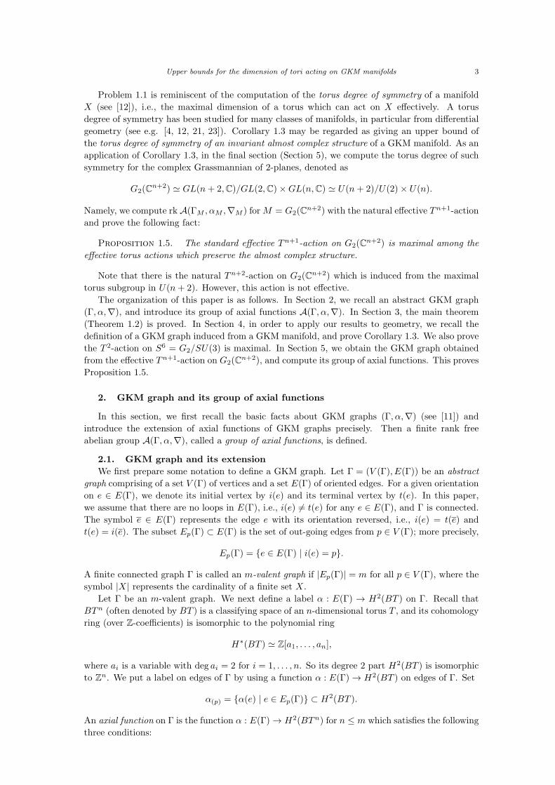
Figure 1 shows examples of GKM graphs. Note that we often omit the axial functions of the

opposite directions of edges (see the 3rd figure) because it is automatically determined by axiom

(1) of a GKM graph.

p q

r

a

b

−a

−a+ b

−b a− b

a b

−a− b

−a −b

a+ b a b

c

−b+ c

a− c

−a+ b

Figure 1. Examples of (2,2)-type, (3,2)-type and (3,3)-type GKM graphs from

the left, where a, b (resp. c) are generators of H∗(BT 2) (resp. H∗(BT 3)). For

example, in the (2, 2)-type GKM graph, the axial function is defined by α(pq) =

a, α(qr) = −a + b, etc. In the (3, 3)-type GKM graph, we omit the axial

functions of the opposite directions of edges. Note that in the figure we do not

distinct two edges e and e, and represent it by one undirected edge.

We note the following lemma proved in [11, Proposition 2.1.3].

Lemma 2.3. Let (Γ, α,∇) be a GKM graph. If α(p) is three-independent for every p ∈ V (Γ),

the connection ∇ is uniquely determined.

Upper bounds for the dimension of tori acting on GKM manifolds 5

Here, in Lemma 2.3, the set of vectors α(p) in H2(BT ) is called three-independent if every

triple {α(ei), α(ej), α(ek)} ⊂ α(p) is linearly independent (e.g., the right (3,3)-type GKM graph

in Figure 1). So, in this case, we may denote (Γ, α,∇) as (Γ, α) without the connection ∇.

We also note the following lemma:

Lemma 2.4. For all e ∈ E(Γ), ce(e) = −2.

Proof. By the axiom (1), (3)-(2) and (3)-(3) of axial function, it is straightforward. □

Remark 2.5. As we mentioned before, ce(e′) represents the Chern number of the line bundle

over the 2-sphere corresponding to e and e′. The sign of this number depends on the choice of the

complex structure on the line bundle. The number ce(e) corresponds to the Chern number of the

tangent bundle of the 2-sphere. In our convention, we take the orientation which gives its Chern

number as −2.

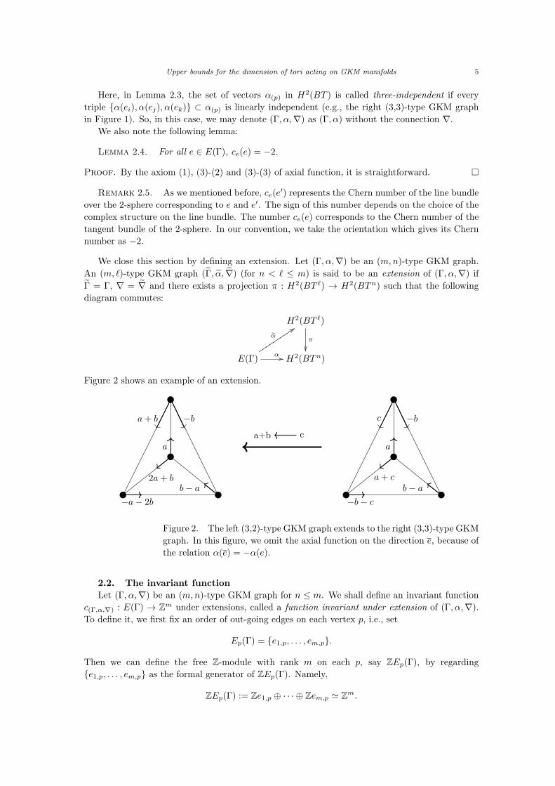
We close this section by defining an extension. Let (Γ, α,∇) be an (m,n)-type GKM graph.

An (m, ℓ)-type GKM graph (Γ, α, ∇) (for n < ℓ ≤ m) is said to be an extension of (Γ, α,∇) if

Γ = Γ, ∇ = ∇ and there exists a projection π : H2(BT ℓ) → H2(BTn) such that the following

diagram commutes:

H2(BT ℓ)

π

��E(Γ)

α

::ttttttttttα // H2(BTn)

Figure 2 shows an example of an extension.

2a+ b

a

a+ b −b

−a− 2b

b− a

a+b c

a+ c

a

c −b

−b− c

b− a

Figure 2. The left (3,2)-type GKM graph extends to the right (3,3)-type GKM

graph. In this figure, we omit the axial function on the direction e, because of

the relation α(e) = −α(e).

2.2. The invariant function

Let (Γ, α,∇) be an (m,n)-type GKM graph for n ≤ m. We shall define an invariant function

c(Γ,α,∇) : E(Γ) → Zm under extensions, called a function invariant under extension of (Γ, α,∇).

To define it, we first fix an order of out-going edges on each vertex p, i.e., set

Ep(Γ) = {e1,p, . . . , em,p}.

Then we can define the free Z-module with rank m on each p, say ZEp(Γ), by regarding

{e1,p, . . . , em,p} as the formal generator of ZEp(Γ). Namely,

ZEp(Γ) := Ze1,p ⊕ · · · ⊕ Zem,p ≃ Zm.

6 S. Kuroki

As an order on each Ep(Γ) is fixed, the connection ∇e : Ei(e)(Γ) → Et(e)(Γ) induces a permutation

on {1, . . . ,m}. So, there is a permutation σ : {1, . . . ,m} → {1, . . . ,m} such that

∇e(ej,i(e)) = eσ(j),t(e).

Then, the connection ∇e defines the isomorphism

Ne : ZEi(e)(Γ) → ZEt(e)(Γ) ∈ GL(m;Z)(2.2)

by the inverse (or equivalently the transpose) of the permutation (m ×m)-square matrix. More

precisely, the square matrix Ne is defined as follows. If we put ZEi(e)(Γ) = Ze1,p⊕· · ·⊕Zem,p (p =

i(e)) and ZEt(e)(Γ) = Ze1,q ⊕ · · · ⊕ Zem,q (q = t(e)), then ∇e induces the following isomorphism:

k1e1,p ⊕ · · · ⊕ kmem,p

7→ k1eσ(1),q ⊕ · · · ⊕ kmeσ(m),q = kσ−1(1)e1,q ⊕ · · · ⊕ kσ−1(m)em,q.

Thus Ne : ZEi(e)(Γ) → ZEt(e)(Γ) is defined by the square matrix which induces the following

isomorphism

Ne :

k1...

km

7→

kσ−1(1)

...

kσ−1(m)

(2.3)

where σ is the permutation induced from ∇e. Take an edge e ∈ E(Γ). Recall that the congruence

coefficient ce(e′) which is defined by (2.1) is an integer attached on every edge e′ ∈ Ei(e)(Γ) for the

fixed edge e ∈ E(Γ). Therefore, the m-tuple of congruence coefficients on e defines the element in

ZEi(e)(Γ) by

ce = (ce(e1,i(e)), . . . , ce(em,i(e))) ∈ Ze1,i(e) ⊕ · · · ⊕ Zem,i(e).

Thus we may define the function

c(Γ,α,∇) : E(Γ) → Zm by c(Γ,α,∇)(e) = ce.

Due to the following proposition (see also [19]), we call this function c(Γ,α,∇) a function invari-

ant under extension of (Γ, α,∇):

Proposition 2.6. For any extension (Γ, α,∇) of (Γ, α,∇), the equation c(Γ,α,∇) = c(Γ,α,∇)

holds.

Proof. Let (Γ, α,∇) be an (m, ℓ)-type GKM graph for some ℓ > n, and ce(e′) be its congruence

coefficient of e′ on e. Fix an order of out-going edges on each vertex p. By the definition of

the function c(Γ,α,∇), it is enough to prove the equation ce(e′) = ce(e

′) for all e ∈ E(Γ) and

e′ ∈ Ei(e)(Γ).

By definition, there is a projection π : H2(BT ℓ) → H2(BTn) such that π ◦ α = α. Together

with the congruence relations (2.1), we have

π(α(∇e(e′))) = α(∇e(e

′)) = α(e′) + ce(e′)α(e)

and

π(α(∇e(e′))) = π(α(e′) + ce(e

′)α(e))

= π(α(e′)) + ce(e′)π(α(e))

= α(e′) + ce(e′)α(e).

Comparing these equations, we establish the statement. □

Upper bounds for the dimension of tori acting on GKM manifolds 7

The following lemma tells us that c(Γ,α,∇)(e) is automatically determined by c(Γ,α,∇)(e) and

Ne defined in (2.2).

Lemma 2.7. For any e ∈ E(Γ), the equation Ne(c(Γ,α,∇)(e)) = c(Γ,α,∇)(e) holds.

Proof. Let σ be the permutation on {1, . . . ,m} induced from ∇e. Then, ∇e(ej,i(e)) = eσ(j),i(e)(and ∇e(eσ(j),i(e)) = ej,i(e)). Therefore, by definitions of Ne and c(Γ,α,∇), it is enough to show the

following equality: ce(eσ−1(j),i(e)) = ce(ej,i(e)), i.e.,

ce(ej,i(e)) = ce(eσ(j),i(e))

for all j = 1, . . . ,m. Due to the congruence relations (2.1) on e and e, we have

α(∇e(ej,i(e)))− α(ej,i(e)) = ce(ej,i(e))α(e)

= α(eσ(j),i(e))− α(ej,i(e))

and

α(∇e(eσ(j),i(e)))− α(eσ(j),i(e)) = ce(eσ(j),i(e))α(e)

= α(ej,i(e))− α(eσ(j),i(e)).

By these equations and α(e) = −α(e), we establish the statement. □

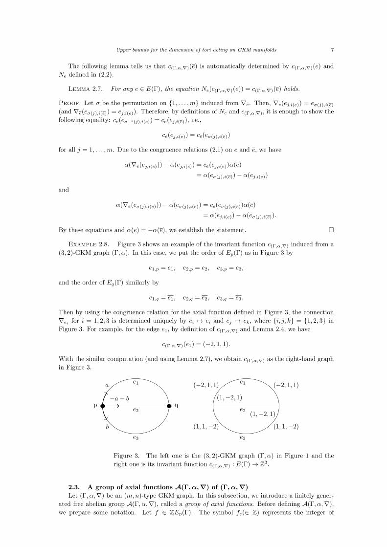
Example 2.8. Figure 3 shows an example of the invariant function c(Γ,α,∇) induced from a

(3, 2)-GKM graph (Γ, α). In this case, we put the order of Ep(Γ) as in Figure 3 by

e1,p = e1, e2,p = e2, e3,p = e3,

and the order of Eq(Γ) similarly by

e1,q = e1, e2,q = e2, e3,q = e3.

Then by using the congruence relation for the axial function defined in Figure 3, the connection

∇ei for i = 1, 2, 3 is determined uniquely by ei 7→ ei and ej 7→ ek, where {i, j, k} = {1, 2, 3} in

Figure 3. For example, for the edge e1, by definition of c(Γ,α,∇) and Lemma 2.4, we have

c(Γ,α,∇)(e1) = (−2, 1, 1).

With the similar computation (and using Lemma 2.7), we obtain c(Γ,α,∇) as the right-hand graph

in Figure 3.

p q

a

−a− b

b

e1

e2

e3

(−2, 1, 1)

(1,−2, 1)

(1, 1,−2)

e1

e2

e3

(−2, 1, 1)

(1,−2, 1)

(1, 1,−2)

Figure 3. The left one is the (3, 2)-GKM graph (Γ, α) in Figure 1 and the

right one is its invariant function c(Γ,α,∇) : E(Γ) → Z3.

2.3. A group of axial functions A(Γ, α,∇) of (Γ, α,∇)

Let (Γ, α,∇) be an (m,n)-type GKM graph. In this subsection, we introduce a finitely gener-

ated free abelian group A(Γ, α,∇), called a group of axial functions. Before defining A(Γ, α,∇),

we prepare some notation. Let f ∈ ZEp(Γ). The symbol fe(∈ Z) represents the integer of

8 S. Kuroki

the coefficient in f corresponding to the edge e ∈ Ep(Γ). For example, if we put the order

Ep(Γ) = {e1, . . . , em} and f = (x1, . . . , xm) ∈ Zm ≃ ZEp(Γ) with respect to this order, then we

put fej = xj .

Definition 2.9 (Group of axial functions). A Z-module A(Γ, α,∇) is defined by the

submodule of

{f : V (Γ) → Zm} =⊕

p∈V (Γ)

ZEp(Γ) ≃⊕

p∈V (Γ)

Zm

which satisfies the following relations for all e ∈ E(Γ):

Ne(f(p))− f(q) = f(q)ec(Γ,α,∇)(e)(2.4)

where i(e) = p, t(e) = q, Ne : ZEp(Γ) → ZEq(Γ) is the square matrix defined in (2.3) and

f(q)e ∈ Z is the integer defined just before. This module A(Γ, α,∇) is said to be a group of axial

functions of (Γ, α,∇) (also see Remark 3.5).

Remark 2.10. As the set {f : V (Γ) → Zm} is a finitely generated free Z-module with rank

m|V (Γ)| i.e., a free abelian group with finite rank, its submodule A(Γ, α,∇) is so too. It is also

easy to check that two groups of axial functions with different orders for Ep(Γ) (for any p ∈ V (Γ))

are isomorphic.

Remark 2.11. The geometric idea behind the definition of the group of axial functions is as

follows: one essentially needs to define the set of all possible weights of a generic circle action (the

circle being a subcircle of the maximal torus action which can act on a GKM manifold) making

sure that the Chern number of the line bundles, in which the tangent bundle splits over each

invariant sphere, stay the same.

The following corollary follows immediately from Definition 2.9 and Proposition 2.6:

Corollary 2.12. Let (Γ, α,∇) be a GKM graph and (Γ, α,∇) be its extension. Then the

two groups of axial functions are isomorphic, i.e., A(Γ, α,∇) ≃ A(Γ, α,∇).

We note the following property of equation (2.4) which will be useful to compute A(Γ, α,∇).

Lemma 2.13. Let f : V (Γ) → Zm be any function. If equation (2.4) holds for some edge

e ∈ E(Γ), then f(p)e = −f(q)e and equation (2.4) also holds for the edge e, where p = i(e) and

q = t(e).

Proof. Let e = ej,p and e = eσ(j),q, where σ is the permutation induced from ∇e. Put

f(p) =

k1,p...

km,p

.

Then f(p)e = kj,p and

Ne(f(p)) =

x1

...

xm

=

kσ−1(1),p

...

kσ−1(m),p

.

This shows that Ne(f(p))e = xσ(j) = kj,p = f(p)e. Therefore, together with Lemma 2.4, we have

Ne(f(p))e − f(q)e = f(p)e − f(q)e = −2f(q)e.

So f(p)e = −f(q)e. Note that Ne = N−1e because ∇e = ∇−1

e . Thus, evaluating equation (2.4) by

Upper bounds for the dimension of tori acting on GKM manifolds 9

Ne and using Lemma 2.7, we have

f(p)−Ne(f(q)) = −f(p)eNe(c(Γ,α,∇)(e)) = −f(p)ec(Γ,α,∇)(e).

This establishes the statement. □

Example 2.14. Before proving the main theorem, let us compute A(Γ, α,∇) of (Γ, α,∇) in

Example 2.8. By the definition of A(Γ, α,∇), we first have

A(Γ, α,∇) = {f : {p, q} → Z3 | Nei(f(p))− f(q) = f(q)eic(Γ,α,∇)(ei)}.

Put f(p) = (x, y, z) ∈ ZEp(Γ) and f(q) = (x′, y′, z′) ∈ ZEq(Γ). Then by Lemma 2.13 x′ = −x,

y′ = −y and z′ = −z. Therefore, for example for the case when i = 1, the relation of A(Γ, α,∇)

says that 1 0 0

0 0 1

0 1 0

x

y

z

−

−x

−y

−z

= −x

−2

1

1

Hence, we also have the relation x + y + z = 0. Similarly, computing for the other edges e2, e3(Lemma 3.2 proved later may also be useful), we get

A(Γ, α,∇) = {(f(p), f(q)) = ((x, y, z), (−x,−y,−z)) | x+ y + z = 0}(≃ Z2).

3. Main theorem

In this section, we prove the following main theorem.

Theorem 3.1. Let (Γ, α,∇) be an (m,n)-type GKM graph. Then the following two state-

ments are equivalent:

1. there is an (m,ℓ)-type GKM graph which is an extension of (Γ, α,∇) for some ℓ ≥ n;

2. ℓ ≤ rk A(Γ, α,∇)(≤ m).

In particular, if rk A(Γ, α,∇) = k, then there is an extended (m,k)-type GKM graph (Γ, α,∇)

which is the maximal among extensions.

3.1. Proof of (1) ⇒ (2)

We first prove (1) ⇒ (2) in Theorem 3.1. The following lemma is the key lemma:

Lemma 3.2. Let (Γ, α,∇) be an (m,n)-type GKM graph. Then, the rank of A(Γ, α,∇)

satisfies the following inequality:

n ≤ rk A(Γ, α,∇) ≤ m.

Proof. We first prove the inequality rk A(Γ, α,∇) ≤ m. By definition, f ∈ A(Γ, α,∇) ⊂⊕p∈V (Γ)ZEp(Γ). Under the same notation as in equation (2.4), we put

f(p) =

x1

...

xm

, f(q) =

y1...

ym

, c(Γ,α,∇)(e) =

k1,p...

km,p

where xj , yj are variables and kj,p ∈ Z for all j = 1, . . . , m. Put f(p)e = xj . Then by equation

(2.4) for e, for all i = 1, . . . , m the following equation holds:

yσ(i) − xi = xjki,p,

where σ is the permutation on {1, . . . ,m} induced from ∇e. This implies that once we choose the

value f(p) ∈ Zm for a vertex p which is connected to q by an edge, then the value f(q) ∈ Zm is

10 S. Kuroki

automatically and uniquely determined. Since Γ is a connected graph, iterating this argument on

each edge, we can determine the value f(r) uniquely for all r ∈ V (Γ) if we choose a value for f(p).

This implies that the restriction map

ρp : A(Γ, α,∇) → Zm such that ρp(f) = f(p)(3.1)

is the injective homomorphism for any vertex p ∈ V (Γ), which proves rk A(Γ, α,∇) ≤ m.

We next prove the next inequality n ≤ rk A(Γ, α,∇). As (Γ, α,∇) is an (m,n)-type GKM

graph, taking a linear basis of H2(BTn) as {a1, . . . , an}, its axial function can be written as

α : E(Γ) → H2(BTn) = Za1 ⊕ · · · ⊕ Zan ≃ Zn. Let πi : H2(BTn) → Zai be the projection onto

the ith coordinate of H2(BTn) with respect to this basis. Define

αi : E(Γ)α−→ H2(BTn)

πi−→ Zai.

Recall that we chose an order on Ep(Γ) = {e1,p, . . . , em,p} for each p ∈ V (Γ). Let

αi(ej,p) = k(i)j,pai

for some k(i)j,p ∈ Z. Then the map fi : V (Γ) → Zm is defined by

fi(p) =

k(i)1,p...

k(i)m,p

∈ ZEp(Γ) ≃ Zm,

for each p ∈ V (Γ). We claim that fi ∈ A(Γ, α,∇) and {f1, . . . , fn} spans the rank n submodule in

A(Γ, α,∇). Let p = i(e), q = t(e) ∈ V (Γ) for some e ∈ E(Γ). In order to prove fi ∈ A(Γ, α,∇),

by definition, it is enough to show the equation

Ne(fi(p))− fi(q) = fi(q)ec(Γ,α,∇)(e).(3.2)

Now we have

α(∇e(ej,p)) = α(eσ(j),q) = α(ej,p) + ce(ej,p)α(e).

Taking πi on these equations, we obtain

αi(∇e(ej,p)) = k(i)σ(j),qai = k

(i)j,pai + ce(ej,p)k

(i)e ai

for all j = 1, . . . ,m, where k(i)e ai = αi(e) = fi(p)eai. Therefore, we havek(i)σ(1),q

...

k(i)σ(m),q

=

k(i)1,p...

k(i)m,p

+ k(i)e

ce(e1,p)...

ce(em,p)

As Ne = N−1

e (where Ne is defined by ∇e), we have the following from this equation:

Ne(fi(q)) = fi(p) + fi(p)ec(Γ,α,∇)(e).

Thus, by multiplying Ne and using Lemma 2.7, we have that

Ne(fi(p))− fi(q) = −fi(p)ec(Γ,α,∇)(e).

Now, by the definition of αi, we have that fi(p)e = −fi(q)e. Hence, we obtain equation (3.2) and

establish that fi ∈ A(Γ, α,∇) for all i = 1, . . . , n. Now, by definition of the effective axial function,

the collection {α(ep,1), . . . , α(ep,m)} spans H2(BTn) ≃ Zn for each p ∈ V (Γ). This implies that for

every p ∈ V (Γ) there is a collection {f1(p), . . . , fn(p)} which spans some n-dimensional subspace

Upper bounds for the dimension of tori acting on GKM manifolds 11

in ZEp(Γ)(≃ Zm). Since the restriction map (3.1) is injective, this also implies that the set of

functions {f1, . . . , fn} spans some n-dimensional submodule in A(Γ, α,∇)(⊂ Zm). This establishes

that n ≤ rk A(Γ, α,∇). □

Assume that there is an (m, ℓ)-type GKM graph (Γ, α,∇) which is an extension of (Γ, α,∇)

for some n ≤ ℓ ≤ m. Then it easily follows from Corollary 2.12 and Lemma 3.2 that

ℓ ≤ rk A(Γ, α,∇) = rk A(Γ, α,∇) ≤ m.

This establishes the statement (1) ⇒ (2) in Theorem 3.1.

3.2. Proof of (2) ⇒ (1)

We next prove (2) ⇒ (1) in Theorem 3.1 for an (m,n)-type GKM graph (Γ, α,∇). Assume

that

ℓ ≤ rank A(Γ, α,∇)(≤ m)

for some ℓ ≥ n. We shall prove that there exists an extension (m, ℓ)-type GKM graph (Γ, α,∇) of

the (m,n)-type GKM graph (Γ, α,∇).

Let f ∈ A(Γ, α,∇). Put the order of Ep(Γ) as {e1,p, . . . , em,p} for p ∈ V (Γ) and

f(p) =

k1,p...

km,p

with respect to this order. Then we may define αa

f : E(Γ) → Za for every a ∈ H2(BTn) by

αaf (ej,p) = kj,pa.

We call this label αaf on edges an a-labeling induced from f ∈ A(Γ, α,∇). From the proof of

Lemma 3.2, it is easy to see that αi := πi ◦ α = αai

fifor i = 1, . . . , n. Therefore, we obtain the

following corollary from the proof of Lemma 3.2, which is the key fact to prove (2) ⇒ (1) and tells

us that the axial function α can be recovered from A(Γ, α,∇) by using αaf .

Corollary 3.3. Let (Γ, α,∇) be an (m,n)-type GKM graph. Then there exists fi ∈A(Γ, α,∇) for i = 1, . . . , n such that {f1, . . . , fn} spans an n-dimensional subspace of A(Γ, α,∇)

and for the fixed basis a1, . . . , an of H2(BTn) the axial function can be split into

α1 ⊕ · · · ⊕ αn = α : E(Γ) → H2(BTn) =n⊕

i=1

Zai

where αi := αai

fiis the ai-labeling induced from fi.

As ℓ ≤ rk A(Γ, α,∇), there are independent elements (as free Z-module)

f1, . . . , fℓ ∈ A(Γ, α,∇).

Moreover, because of ℓ ≥ n, we may choose the first part f1, . . . , fn as the basis induced from

(Γ, α,∇) in Corollary 3.3 (also see the definitions of fi’s in the proof of Lemma 3.2), and put

fi(p) =

k(i)1,p...

k(i)m,p

∈ ZEp(Γ) ≃ Zm,(3.3)

for i = 1, . . . , ℓ and p ∈ V (Γ). Fix the basis of H2(BT ℓ) as a1, . . . , aℓ, where the first n elements

a1, . . . , an are the basis of H2(BTn) (see Corollary 3.3), where Tn ⊂ T ℓ. Let αi be the ai-labeling

12 S. Kuroki

induced from fi, i.e., αi = αai

fi, for i = 1, . . . , ℓ. Then, we can define the function as follows:

α := ⊕ℓi=1αi : E(Γ) → H2(BT ℓ).

The following lemma says that the triple (Γ, α,∇) is a GKM graph extending (Γ, α,∇).

Lemma 3.4. The triple (Γ, α,∇) defined as above is an (m, ℓ)-type GKM graph which is an

extension of an (m,n)-type GKM graph (Γ, α,∇).

Proof. Since α = ⊕ni=1αi and α = α ⊕ (⊕ℓ

i=n+1αi), it is enough to prove that α satisfies the

axioms of a GKM graph under the same connection ∇ of (Γ, α,∇).

We first claim that axiom (1) of a GKM graph holds for α, i.e., α(e) = −α(e). To do this, by the

definition of α, it is enough to show that αi(e) = −αi(e) for all i = 1, . . . , ℓ. Let e = ej,p ∈ Ep(Γ)

and e = eσ(j),q ∈ Eq(Γ) for j = 1, . . . ,m, where i(e) = p, t(e) = q and σ is the permutation on

{1, . . . ,m} induced from ∇e : Eq(Γ) → Ep(Γ). Then by the definition of αi, we have that

αi(e) = αi(ej,p) = k(i)j,pai

and

αi(e) = αi(eσ(j),q) = k(i)σ(j),qai

where fi(p)e = k(i)j,p and fi(q)e = k

(i)σ(j),q ∈ Z. As fi ∈ A(Γ, α,∇), it follows from Lemma 2.13 that

k(i)j,p = −k

(i)σ(j),q. This establishes axiom (1) of a GKM graph.

We next claim condition (4) regarding effectiveness, i.e., α(p) = {α(e) | e ∈ Ep(Γ)} spans

H2(BT ℓ) for all p ∈ V (Γ). Recall that for Ep(Γ) := {e1,p, . . . , em,p},

α(ej,p) = ⊕ℓi=1αi(ej,p) = ⊕ℓ

i=1k(i)j,pai,

where the integer k(i)j,p is the jth coefficient of fi(p) ∈ Zm (see (3.3)). Now {f1, . . . , fℓ} spans

an ℓ-dimensional subspace of A(Γ, α,∇). As the restriction map defined in (3.1) is injective (by

similar arguments as in the proof of Lemma 3.2), we have that the subset {f1(p), . . . , fℓ(p)} ⊂ Zm

also spans a subgroup which is isomorphic to Zℓ for all p ∈ V (Γ). This shows that the (m × ℓ)-

matrix (k(i)j,p)i,j has rank ℓ(≤ m) and some minor (of (ℓ×ℓ)-smaller square matrix in (k

(i)j,p)i,j) with

determinant ±1, for all p ∈ V (Γ). Therefore, there are ℓ elements in α(p) = {α(e1,p), . . . , α(em,p)}which generate H2(BT ℓ). This establishes condition (4).

We also check axiom (2), i.e., α(p) is pairwise linearly independent for all p ∈ V (Γ). As α is

an axial function, α(p) is pairwise linearly independent for all p ∈ V (Γ), i.e., α(e) and α(e′) are

linearly independent for all pairs e, e′ ∈ Ep(Γ). Moreover, we may write

α(e) = ⊕ℓi=1αi(e) = ⊕n

i=1αi(e)⊕ (⊕ℓi=n+1αi(e)) = α(e)⊕ (⊕ℓ

i=n+1αi(e)),

and

α(e′) = ⊕ℓi=1αi(e

′) = ⊕ni=1αi(e

′)⊕ (⊕ℓi=n+1αi(e

′)) = α(e′)⊕ (⊕ℓi=n+1αi(e

′)).

Here, by definition of αi, the element αi(e) (resp. αi(e′)), for i = n + 1, . . . , ℓ, is independent

with respect to α(e) (resp. α(e′)). Hence, we have that α(e) and α(e′) are also pairwise linearly

independent. This establishes axiom (2).

Finally, we claim axiom (3), i.e., α satisfies the following congruence relation: for each e′ ∈Ei(e)(Γ)

α(∇e(e′)) = α(e′) + ce(e

′)α(e),

Upper bounds for the dimension of tori acting on GKM manifolds 13

where ce(e′) is the integer that satisfies

α(∇e(e′)) = α(e′) + ce(e

′)α(e).

Since α = ⊕ℓi=1αi, it is enough to prove that αi satisfies the congruence relation:

αi(∇e(e′)) = αi(e

′) + ce(e′)αi(e).

Set e = ej,p and e′ = eh,p for some j, h = 1, . . . ,m, and ∇e(e′) = eσ(h),q. By definition, αi(ej,p) =

k(i)j,pai. Therefore, it is enough to check the following relation:

k(i)σ(h),q = k

(i)h,p + ce(e

′)k(i)j,p.(3.4)

Using fi ∈ A(Γ, α,∇), (i.e., equation (2.4) holds), Lemma 2.7 and Lemma 2.13, we have

Ne(fi(p))− fi(q) = −fi(p)eNe(c(Γ,α,∇)(e))(3.5)

for all i = 1, . . . , ℓ. Since e = ej,p, we have fi(p)e = k(i)j,p (see (3.3)). Therefore, equation (3.5)

implies that k(i)σ−1(1),p

...

k(i)σ−1(m),p

−

k(i)1,q...

k(i)m,q

= −k(i)j,p

ce(eσ−1(1),p)...

ce(eσ−1(m),p)

.

This shows that

k(i)h,p − k

(i)σ(h),q = −k

(i)j,pce(eh,p).

Since e′ = eh,p, this equation establishes equation (3.4).

Consequently, α is an extended axial function of α. □

This establishes (2) ⇒ (1) in Theorem 3.1. Together with Section 3.1, we obtain Theorem 3.1.

Remark 3.5. Lemma 3.4 tells us that from an element of A(Γ, α,∇) we can construct

an extension of (Γ, α,∇). In fact, by similar arguments, we see that A(Γ, α,∇) contains every

extension of (Γ, α,∇), i.e., every extension of (Γ, α,∇) corresponds to an element of A(Γ, α,∇).

Furthermore, it is not so difficult to show that every axial function on Γ whose connection is ∇can be constructed by an element of A(Γ, α,∇). This is the reason why we call A(Γ, α,∇) a group

of axial functions.

As a corollary, we have the following fact.

Corollary 3.6. Let (Γ, α,∇) be an (m,n)-type GKM graph. If one of the following cases

hold, then there are no extensions of (Γ, α,∇):

1. m = n;

2. rk A(Γ, α,∇) = n.

Example 3.7. By Corollary 3.6 and the computation in Example 2.14, the GKM graphs in

Figure 1 have no extensions, i.e., they are the maximal GKM graphs.

4. Applications to geometry

Guillemin-Zara studied GKM graphs as a combinatorial counter part to GKM manifolds, and

they built a bridge between the geometry (in particular, symplectic) of GKM manifolds and the

combinatorics of GKM graphs. In this and the next sections, we give a new application of GKM

14 S. Kuroki

graphs to study the geometry of GKM manifolds. More precisely, we apply our main result to

study the maximal torus actions of GKM manifolds.

4.1. GKM manifold and its GKM graph

We first briefly recall the relation between GKM manifolds and GKM graphs (see [11] for

details). Let M be a 2m-dimensional, compact, connected smooth manifold with an effective

n-dimensional torus Tn-action, where 1 ≤ n ≤ m. We often denote such a manifold by (M,T ) or

(M,T, φ) if we emphasize the action φ : T × M → M . Denote by M1 ⊂ M the set of elements

x ∈ M such that the orbit T (x) = {x} (a fixed point) or T (x) ≃ S1, i.e.,

M1 = {x ∈ M | dimT (x) ≤ 1}.

The set M1 is called the one-skeleton of (M,T ).

A 2m-dimensional manifold with an n-dimensional torus action (M,T ) is said to be a GKM

manifold or an (m,n)-type GKM manifold if the following three conditions hold:

1. MT = ∅;

2. the manifold M has a T -invariant almost complex structure;

3. the one-skeleton of M has the structure of an abstract (connected) graph ΓM such that its

vertices V (ΓM ) are the fixed points and its edges E(ΓM ) are embedded 2-spheres connecting

two fixed points.

Remark 4.1. The third condition implies that the orbit space of the one-skeleton is one-

dimensional. Therefore, together with condition (1), the set of fixed points MT is always isolated.

Moreover, by definition of the (m,n)-type GKM manifold M , if dimT (= n) = 1 then M is

equivariantly diffeomorphic to CP 1 with a non-trivial S1-action. So, in this paper, we often

assume 2 ≤ n ≤ m for an (m,n)-type GKM manifold. We also do not assume the equivariant

formality because we do not use the equivariant cohomolgy of GKM manifolds.

Due to [11], the GKM manifold M defines the GKM graph (ΓM , αM ,∇M ) by using its one-

skeleton and the tangential representations. In this paper, such a GKM graph (ΓM , αM ) (or

(ΓM , αM ,∇M )) is called an induced GKM graph from M .

Example 4.2. In Figure 1, the left GKM graph is the GKM graph induced from the standard

T 2-action on CP 2 and the right one is that induced from T 3-action on CP 3. The middle GKM

graph is induced from the T 2-action on S6 = G2/SU(3), where G2 is the exceptional Lie group,

see [9, Section 5.2].

4.2. Extensions of torus actions

The definition of an extension of GKM graphs in Section 2.1 is motivated by an extension of

a torus action on a GKM manifold. We explain it more precisely in this section.

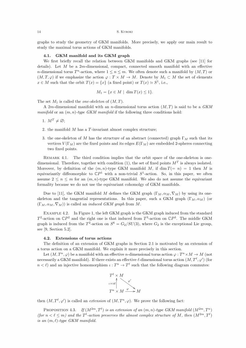
Let (M,Tn, φ) be a manifold with an effective n-dimensional torus action φ : Tn×M → M (not

necessarily a GKMmanifold). If there exists an effective ℓ-dimensional torus action (M,T ℓ, φ′) (for

n < ℓ) and an injective homomorphism ι : Tn → T ℓ such that the following diagram commutes:

T ℓ ×Mφ′

##HHH

HHHH

HH

Tn ×M

ι×id

OO

φ // M

then (M,T ℓ, φ′) is called an extension of (M,Tn, φ). We prove the following fact:

Proposition 4.3. If (M2m, T ℓ) is an extension of an (m,n)-type GKM manifold (M2m, Tn)

(for n < ℓ ≤ m) and the T ℓ-action preserves the almost complex structure of M , then (M2m, T ℓ)

is an (m, ℓ)-type GKM manifold.

Upper bounds for the dimension of tori acting on GKM manifolds 15

Furthermore, the induced (m, ℓ)-type GKM graph (ΓM , αM , ∇M ) from (M,T ℓ) is an extension

of the induced (m,n)-type GKM graph (ΓM , αM ,∇M ) from (M,Tn).

Proof. Since the T ℓ-action preserves the almost complex structure of M , it is enough to check

that its one-skeleton has the structure of a graph. We note that for all p ∈ M two orbits of p of

these actions satisfy Tn(p) ⊂ T ℓ(p), because the T ℓ-action is an extension of Tn-action.

We first claim that MTn

= MT ℓ

. Because Tn(p) ⊂ T ℓ(p) for all p ∈ M , we have that

MTn ⊃ MT ℓ

. Assume that there exists a fixed point p ∈ MTn

such that T ℓ(p) = {p}. As is well-

known, there is a decomposition TpM = TpTℓ(p)⊕NpT

ℓ(p), where TpTℓ(p)( = {0}) is the tangent

space and NpTℓ(p) is the normal space of T ℓ(p) on p. By using the differentiable slice theorem, the

isotropy subgroup T ℓp (of the T ℓ-action on p) acts on TpT

ℓ(p) trivially. This shows that Tn(⊂ T ℓp)

also acts on TpTℓ(p) trivially. However, by the definition of GKM manifolds, for the restricted

action (TpM,Tn), there is another decomposition TpM = ⊕mi=1V (ai) such that each representation

ai : Tn → S1 is non-trivial. This contradicts that Tn acts on ({0} =)TpT

ℓ(p) ⊂ TpM trivially.

Hence, MTn

= MT ℓ

.

Take p ∈ M such that Tn(p) ≃ S1. Since we assume that the one-skeleton of (M,Tn) has

the structure of a connected graph, we have that p is an element in an invariant 2-sphere S2 of

(M,Tn). As MTn

= MT ℓ

, by considering the tangential representation around fixed points on

this Tn-invariant S2(∋ p), there exists a representation ρ : T ℓ → S1 which may be regarded as

the extension of the Tn-action on this S2. Therefore, every Tn-invariant S2 is also a T ℓ-invariant

S2, i.e., if Tn(p) ≃ S1 then T ℓ(p) ≃ S1. Together with Tn(p) ⊂ T ℓ(p) for all p ∈ M , this implies

that the two one-skeletons of (M2m, Tn) and (M2m, T ℓ) are the same.

We next prove the final statement. By arguments similar to the above, we have ΓM = ΓM .

Moreover, because the extended T ℓ-action preserves the Tn-invariant almost complex structure,

the splitting ⊕mi=1Li, of the restriction of the tangent bundle to such as S2, by the Tn-action is also

preserved by the extended T ℓ-action. This implies that the two connections on the induced GKM

graphs ∇M from the Tn-action and ∇M from the extended T ℓ-action are the same. Finally, put

the induced homomorphism from the inclusion ι : Tn → T ℓ as π : H2(BT ℓ) → H2(BTn). Then

by considering the tangential representations (of both Tn and T ℓ-actions) around fixed points, it

is easy to check that there is the following commutative diagram:

H2(BT ℓ)

π

��E(ΓM )

αM

99ssssssssssαM // H2(BTn)

This establishes the final statement. □

Therefore, by using Theorem 3.1 (or Theorem 1.2) and Proposition 4.3, we have Corollary 1.3.

4.3. Maximal torus action on S6 = G2/SU(3)

As we mentioned in Example 4.2, the (3, 2)-type GKM graph in Figure 1 is the induced GKM

graph of the GKM manifold (G2/SU(3), T 2), where T 2 acts on G2 as its maximal torus subgroup

(e.g. see [9]). We also note that G2/SU(3) ≃ S6 (diffeomorphic). Therefore, by using Corollary 1.3

and Example 2.14, the following well-known fact can be proved (see also [3]):

Corollary 4.4. The T 2-action on G2/SU(3) ≃ S6 is the maximal torus action. In other

words, there are no extended T 3-actions on S6 of this T 2-action, which preserves the almost

complex structure induced from the homogeneous space G2/SU(3).

Remark 4.5. Note that there is the T 3-action on S6 ⊂ C3 ⊕ R defined by the standard

T 3-action on C3 (see e.g. [15]). However, from Corollary 4.4, this action is not the extended action

of the T 2-action on S6 = G2/SU(3).

In the next section, we shall apply our results for more complicated GKM manifolds.

16 S. Kuroki

5. Maximal torus action on the complex Grassmannian G2(Cn+2)

The (complex) Grassmannian (of 2-planes in Cn+2), denoted by G2(Cn+2), is defined by the

set of all complex 2-dimensional vector spaces in Cn+2. Namely,

G2(Cn+2) := {V ⊂ Cn+2 | dimC V = 2}.(5.1)

The Grassmannian G2(Cn+2) has the natural transitive SU(n + 2)-action which is induced from

the standard SU(n+ 2)-action on Cn+2. Since its isotropy group is S(U(2)×U(n)), G2(Cn+2) is

diffeomorphic to the homogeneous space SU(n+2)/S(U(2)×U(n)) (also see [13]). In particular,

this shows that

dimG2(Cn+2) = dimSU(n+ 2)/S(U(2)× U(n)) = 4n.

Since a maximal torus of SU(n + 2) is isomorphic to Tn+1, there is a restricted Tn+1-action on

G2(Cn+2) and its one-skeleton has the structure of a graph (see [9]). We denote this action by

(SU(n+2)/S(U(2)×U(n)), Tn+1). Note that the action (SU(n+2)/S(U(2)×U(n)), Tn+1) is not

effective because there is the non-trivial center in SU(n+2) (isomorphic to Z/(n+2)Z); therefore,the GKM graph obtained from this action does not satisfy condition (4) in Section 2, i.e., the axial

function is not an effective axial function. So, in this paper, we define the Tn+1-action onG2(Cn+2)

by the induced action from the standard Tn+1-action on the first (n+1)-coordinates in Cn+2 (see

(5.1)). We denote this action as (G2(Cn+2), Tn+1). It is easy to check that (G2(Cn+2), Tn+1)

is effective and preserves the complex structure of G2(Cn+2) induced from that of Cn+2. For

example, when n = 1, (G2(C3), T 2) is equivariantly diffeomorphic to the complex projective space

CP 2 with the standard T 2-action, i.e., the toric manifold. Note that, for n ≥ 2, (G2(Cn+2), Tn+1)

is not a toric manifold.

Remark 5.1. GKM graphs obtained from the non-effective torus actions for flag manifolds

are studied by Tymoczko in [20] Fukukawa-Ishida-Masuda in [6] etc.

In the next subsection, we compute the GKM graph of (G2(Cn+2), Tn+1). For simplicity, we

put

Mn = G2(Cn+2)

from the next subsection.

Remark 5.2. The following computation of the GKM graph of (G2(Cn+2), Tn+1) is not new.

In [9], the computation of GKM graphs of more general homogeneous spaces are treated. However,

for convenience, we give a precise computation here.

5.1. The GKM graph of (G2(Cn+2), Tn+1)

Let (Γn, αn,∇n) be the induced GKM graph from (Mn, Tn+1). Note that Γn = (V (Γn), E(Γn))

is a 2n-valent graph, because the real dimension of Mn is 4n, where n ≥ 1.

We first consider the fixed points of (Mn, Tn+1). By definition, the Grassmannian Mn may be

identified with the following set:

{[v1, v2] | v1, v2 are linearly independent in Cn+2},

where the symbol [v1, v2] represents the equivalence class such that [v1, v2] is identified with [w1, w2]

if two pairs of vectors {v1, v2} and {w1, w2} span the same 2-dimensional complex vector space in

Cn+2. Under this identification, the element t ∈ Tn+1 acts on [v1, v2] ∈ Mn by

t · [v1, v2] 7→ [tv1, tv2],

where t ∈ Tn+1 acts on v ∈ Cn+2 by the standard coordinatewise multiplication on the first

Upper bounds for the dimension of tori acting on GKM manifolds 17

(n+ 1)-coordinates. Then, the fixed points can be denoted by

MTn := {[ei, ej ] | i = j, i, j = 1, . . . , n+ 2},

where e1, . . . , en+2 are the standard basis in Cn+2. By identifying the element [ei, ej ] ∈ MTn as

the subset {i, j} in [n+ 2] := {1, 2, . . . , n+ 2}, we may regard the set of vertices V (Γn) as

V (Γn) = {{i, j} ⊂ [n+ 2] | i = j}.

We also have that

|V (Γn)| =(n+ 2

2

)=

(n+ 2)(n+ 1)

2.

We next consider the invariant 2-spheres in (Mn, Tn+1). Fix {i, j} ⊂ [n+2]. Now the following

subsets are Tn+1-invariant sets in Mn which contain [ei, ej ]:

Si,ki,j = {[ei, vjk] ∈ Mn | vjk = ajej + akek, (aj , ak) ∈ C2 \ {0}};

Sj,ki,j = {[vik, ej ] ∈ Mn | vik = aiei + akek, (ai, ak) ∈ C2 \ {0}},

for all k ∈ [n+ 2] \ {i, j}.As [ei, vjk] and [ei, λvjk] (for all λ ∈ C∗) are the same element in Mn, we have that Si,k

i,j is

diffeomorphic to CP 1. Similarly, Sj,ki,j is also diffeomorphic to CP 1. Moreover, [ei, ej ], [ei, ek] ∈ Si,k

i,j

and [ei, ej ], [ek, ej ] ∈ Sj,ki,j . This shows that if {i, j} ∩ {k, l} = ∅ then the fixed points [ei, ej ] and

[ek, el] are on the same invariant 2-sphere. Namely, the pair of two distinct sets {i, j} and {k, l} suchthat {i, j}∩ {k, l} = ∅ may be regarded as an edge of the GKM graph, i.e., an element in E(Γn).

We call the edge corresponding to Si,ki,j (resp. Sj,k

i,j ) as Ei,ki,j ∈ E(Γn) (resp. Ej,k

i,j ∈ E(Γn)). Note

that for all k ∈ [n+ 2] \ {i, j}, Ei,ki,j and Ej,k

i,j are out-going edges from {i, j}. Since dimMn = 4n,

the number of out-going edges from {i, j} is 2n. Hence, the set of all out-going edges from {i, j}can be denoted by

E{i,j}(Γn) = {Ei,ki,j , E

j,ki,j | k ∈ [n+ 2] \ {i, j}}.

Figure 4 shows the one-skeleton induced from G2(C4).

{2, 4}

{1, 2}

{2, 3}

{1, 3}

{3, 4}

{1, 4}

E1,41,2

E1,21,4

Figure 4. The vertices and edges of the one-skeleton of the Grassmannian G2(C4).

Next we consider the tangential representations around fixed points. To do that, we use the

following notations:

18 S. Kuroki

• the symbol E(η) represents the total space of the fibre bundle η over Mn;

• the symbol ηp is the restriction of η onto p ∈ Mn;

Recall the structure of the tangent bundle τ of Mn. Let ϵn+2C be the trivial bundle E(ϵn+2

C ) =

Mn × Cn+2 → Mn. Then, the tautological vector bundle γ over Mn is defined as follows:

E(γ) = {(V, x) ∈ Mn × Cn+2 | x ∈ V } → Mn,

where the projection of the bundle is just the projection onto the 1st factor. Note that γ is a

complex 2-dimensional vector bundle overMn and the diagonal Tn+1-action on Mn×Cn+2 induces

the Tn+1-action on E(γ); thus we may regard γ as the Tn+1-equivariant vector bundle. Let γ⊥ be

the normal bundle of γ in ϵn+2C (we define the inner product on Cn+2 as the standard Hermitian

inner product). Since γ is a complex 2-dimensional vector bundle, γ⊥ is a complex n-dimensional

vector bundle. Moreover, since the Tn+1-action on Cn+2 preserves the standard Hermitian inner

product, the diagonal Tn+1-action on Mn × Cn+2 induces the Tn+1-action on γ⊥.

Similar to the case of the real Grassmannian (see [18, Section 5 or proof of Theorem 14.10]), the

tangent bundle τ of Mn is isomorphic to the complex 2n-dimensional vector bundle Hom(γ, γ⊥).

Therefore, the tangent space around [ei, ej ] ∈ MTn may be regarded as

τ[ei,ej ] ≡ Hom(γ[ei,ej ], γ⊥[ei,ej ]

).

Since the total space of γ[ei,ej ] is Vij := {Aiei + Ajej | (Ai, Aj) ∈ C2}, its normal space in Cn+2

consists of

V ⊥ij = {

∑k∈[n+2]\{i,j}

Bkek | Bk ∈ C}.

Therefore, φ ∈ Hom(Vij , V⊥ij ) can be denoted by

φ(Aiei +Ajej) =∑

k∈[n+2]\{i,j}

fk(Ai, Aj)ek

for some linear map fk : C2 → C, i.e., fk(Ai, Aj) = Aiℓik +Ajℓjk for some (ℓik, ℓjk) ∈ C2 (we will

identify fk as (ℓik, ℓjk)). Then, we may regard φ = (fk)k∈[n+2]\{i,j} ∈ M(2, n;C) as the complex

(2 × n)-matrix. Now the Tn+1-actions on γ and γ⊥ induce the Tn+1-action on Hom(γ, γ⊥) as

follows: for φ ∈ Hom(γx, γ⊥x ) (x ∈ Mn) and t ∈ Tn+1,

t · φ = t ◦ φ ◦ t−1 : γtxt−1

−→ γxφ−→ γ⊥

xt−→ γ⊥

tx.

Therefore, on x = [ei, ej ], we have t · fk = (t−1i tkℓik t−1

j tkℓjk) for fk = (ℓik ℓjk), φ = (fk) ∈M(2, n;C) and t = (t1, . . . , tn+1, 1) ∈ Tn+2, i.e., tn+2 = 1. Hence, on the fixed point [ei, ej ] ∈ MT

n ,

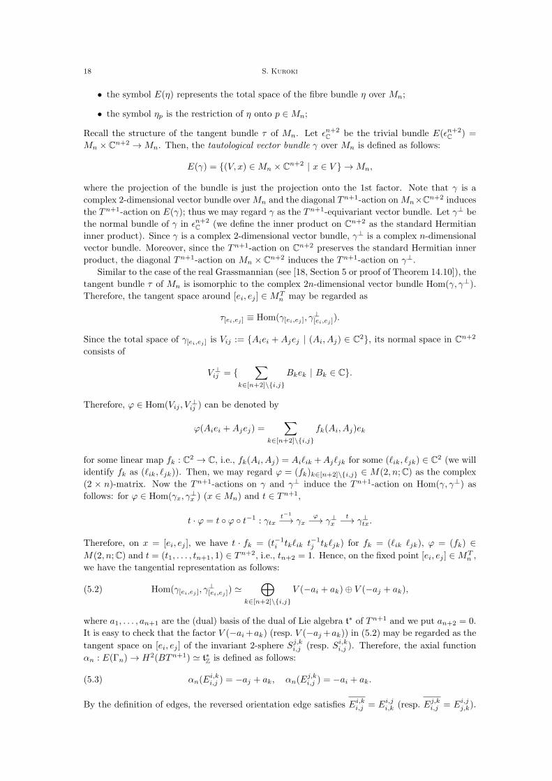
we have the tangential representation as follows:

Hom(γ[ei,ej ], γ⊥[ei,ej ]

) ≃⊕

k∈[n+2]\{i,j}

V (−ai + ak)⊕ V (−aj + ak),(5.2)

where a1, . . . , an+1 are the (dual) basis of the dual of Lie algebra t∗ of Tn+1 and we put an+2 = 0.

It is easy to check that the factor V (−ai+ak) (resp. V (−aj +ak)) in (5.2) may be regarded as the

tangent space on [ei, ej ] of the invariant 2-sphere Sj,ki,j (resp. Si,k

i,j ). Therefore, the axial function

αn : E(Γn) → H2(BTn+1) ≃ t∗Z is defined as follows:

αn(Ei,ki,j ) = −aj + ak, αn(E

j,ki,j ) = −ai + ak.(5.3)

By the definition of edges, the reversed orientation edge satisfies Ei,ki,j = Ei,j

i,k (resp. Ej,ki,j = Ei,j

j,k).

Upper bounds for the dimension of tori acting on GKM manifolds 19

Therefore, by the definition of the axial function the following equation holds:

αn(Ei,ji,k) = −ak + aj = −αn(E

i,ki,j ) (resp. αn(E

i,jj,k) = −ak + ai = −αn(E

j,ki,j )).

We finally compute a connection on (Γn, αn). Put the connection on the edge Ei,ki,j as

(∇n)Ei,ki,j

= (∇n)i,ki,j . Namely,

(∇n)i,ki,j : E{i,j}(Γn) → E{i,k}(Γn),

where

E{i,j}(Γn) := {Ei,li,j , E

j,li,j | l ∈ [n+ 2] \ {i, j}},

E{i,k}(Γn) := {Ei,li,k, E

k,li,k | l ∈ [n+ 2] \ {i, k}}.

Note that the set of the weights {−ai + ak,−aj + ak | k ∈ [n + 2] \ {i, j}} are 3-independent for

all {i, j} ⊂ [n + 2] (see (5.3)). Therefore, it follows from Lemma 2.3 that the connection ∇n on

(Γn, αn) is unique. This implies that the bijection (∇n)i,ki,j which satisfies the congruence relation

(2.1) is unique. Hence, by computing the congruence relation (2.1) of (Γn, αn), the connection

must be defined as follows:

(∇n)i,ki,j (E

i,ki,j ) = Ei,k

i,j = Ei,ji,k,

(∇n)i,ki,j (E

i,li,j) = Ei,l

i,k for l ∈ [n+ 2] \ {i, j, k},

(∇n)i,ki,j (E

j,li,j) = Ek,l

i,k for l ∈ [n+ 2] \ {i, j, k},

(∇n)i,ki,j (E

j,ki,j ) = Ej,k

i,k .

In addition, we also have that

αn(Ei,li,k)− αn(E

i,li,j) = ci,ki,j (E

i,li,j)αn(E

i,ki,j )

−ak + al − (−aj + al) = ci,ki,j (Ei,li,j)(−aj + ak)

and

αn(Ek,li,k)− αn(E

j,li,j) = ci,ki,j (E

j,li,j)αn(E

i,ki,j )

−ai + al − (−ai + al) = ci,ki,j (Ej,li,j)(−aj + ak),

for l ∈ [n+ 2] \ {i, j, k} and

αn(Ej,ki,k )− αn(E

j,ki,j ) = ci,ki,j (E

j,ki,j )αn(E

i,ki,j )

−ai + aj − (−ai + ak) = ci,ki,j (Ej,ki,j )(−aj + ak),

for some integers (congruence coefficients) ci,ki,j (Ei,li,j), c

i,ki,j (E

j,li,j). Therefore, together with

Lemma 2.4, the congruence coefficients are

ci,ki,j (Ei,ki,j ) = −2,

ci,ki,j (Ei,li,j) = −1 for l ∈ [n+ 2] \ {i, j, k},

ci,ki,j (Ej,li,j) = 0 for l ∈ [n+ 2] \ {i, j, k},

ci,ki,j (Ej,ki,j ) = −1.

In summary we have that

Proposition 5.3. Let Γn = (V (Γn), E(Γn)) be the abstract graph defined by

• the set of vertices V (Γn) consists of all {i, j} in [n+ 2] for i = j;

20 S. Kuroki

• the set of edges E(Γn) consists of all pairs of distinct vertices {i, j}, {k, l} such that {i, j} ∩{k, l} = ∅.

Define its axial function as αn : E(Γn) → H2(BTn+1) in (5.3). Then, the connection ∇n is

uniquely determined (as above) and the triple (Γn, αn,∇n) is the (2n, n+ 1)-type GKM graph.

Remark 5.4. The graph in Proposition 5.3 is known as the Johnson graph J(n+ 2, 2). The

first GKM graph in Figure 1 shows the case when n = 1, i.e., the Johnson graph J(3, 2), and the

GKM graph in Figure 5 shows the case when n = 2, i.e., the Johnson graph J(4, 2). It is known

that the one-skeleton of the general Grassmannian Gk(Cn+k) (for k ≥ 1) is the Johnson graph

J(n+ k, k) (see [1]).

{2, 4}

{1, 2}

{2, 3}

{1, 3}

{3, 4}

{1, 4}

−a1−a1 + a3

−a2 + a3

a3

−a2 + a3

−a2 + a1−a2 + a1

−a1 a2

a2

a3

−a1 + a3

Figure 5. The GKM graph (Γ2, α2,∇2) of (G2(C4), T 3).

5.2. The second main result

Since we fix the axial function αn on Γn and its connection ∇n is unique, we may write the

GKM graph (Γn, αn,∇n) of (Mn, Tn+1) as Γn for simplicity; therefore, we denote the group of

axial functions A(Γn, αn,∇n) as A(Γn). This final section is devoted to the proof of the following

theorem:

Theorem 5.5. The group of axial functions A(Γn) is isomorphic to Zn+1.

When n = 1, the GKM graph Γ1 is the (2, 2)-type GKM graph (which is the first GKM graph

in Figure 1). Therefore, by Theorem 3.1, we have that A(Γ1) ≃ Z2. Hence, we may assume that

n ≥ 2.

To prove Theorem 5.5, we first choose an order on E{i,j}(Γn) for i, j ∈ [n + 2] as follows (see

Figure 6 for n = 2):

• Ei,ki,j ≺ Ej,l

i,j if i < j, where k, l ∈ [n+ 2] \ {i, j};

• Ei,ki,j ≺ Ei,l

i,j if k < l, where k, l ∈ [n+ 2] \ {i, j}.

Take f ∈ A(Γn) and put

f({n+ 1, n+ 2}) =

x1

...

x2n

Upper bounds for the dimension of tori acting on GKM manifolds 21

{2, 4}

{1, 2}

{2, 3}

{1, 3}

{3, 4}

{1, 4}

(1)

(3)

(2)

(4)

(4)

(2)

(3)

(1)

(3)

(1)

(4)

(2)

(3)

(4)

(2)

(1)

(1) (3)

(4)(2)

(3)(1)

(4)

(2)

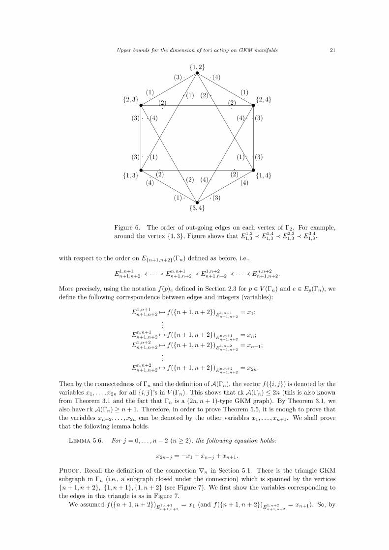
Figure 6. The order of out-going edges on each vertex of Γ2. For example,

around the vertex {1, 3}, Figure shows that E1,21,3 ≺ E1,4

1,3 ≺ E2,31,3 ≺ E3,4

1,3 .

with respect to the order on E{n+1,n+2}(Γn) defined as before, i.e.,

E1,n+1n+1,n+2 ≺ · · · ≺ En,n+1

n+1,n+2 ≺ E1,n+2n+1,n+2 ≺ · · · ≺ En,n+2

n+1,n+2.

More precisely, using the notation f(p)e defined in Section 2.3 for p ∈ V (Γn) and e ∈ Ep(Γn), we

define the following correspondence between edges and integers (variables):

E1,n+1n+1,n+2 7→ f({n+ 1, n+ 2})E1,n+1

n+1,n+2= x1;

...

En,n+1n+1,n+2 7→ f({n+ 1, n+ 2})En,n+1

n+1,n+2= xn;

E1,n+2n+1,n+2 7→ f({n+ 1, n+ 2})E1,n+2

n+1,n+2= xn+1;

...

En,n+2n+1,n+2 7→ f({n+ 1, n+ 2})En,n+2

n+1,n+2= x2n.

Then by the connectedness of Γn and the definition of A(Γn), the vector f({i, j}) is denoted by the

variables x1, . . . , x2n for all {i, j}’s in V (Γn). This shows that rk A(Γn) ≤ 2n (this is also known

from Theorem 3.1 and the fact that Γn is a (2n, n + 1)-type GKM graph). By Theorem 3.1, we

also have rk A(Γn) ≥ n+ 1. Therefore, in order to prove Theorem 5.5, it is enough to prove that

the variables xn+2, . . . , x2n can be denoted by the other variables x1, . . . , xn+1. We shall prove

that the following lemma holds.

Lemma 5.6. For j = 0, . . . , n− 2 (n ≥ 2), the following equation holds:

x2n−j = −x1 + xn−j + xn+1.

Proof. Recall the definition of the connection ∇n in Section 5.1. There is the triangle GKM

subgraph in Γn (i.e., a subgraph closed under the connection) which is spanned by the vertices

{n+ 1, n+ 2}, {1, n+ 1}, {1, n+ 2} (see Figure 7). We first show the variables corresponding to

the edges in this triangle is as in Figure 7.

We assumed f({n + 1, n + 2})E1,n+1n+1,n+2

= x1 (and f({n + 1, n + 2})E1,n+2n+1,n+2

= xn+1). So, by

22 S. Kuroki

{1, n+ 1} {1, n+ 2}

{n+ 1, n+ 2}

xn+1 − x1

−x1

x1 − xn+1

−xn+1

xn+1x1

Figure 7. The triangle GKM subgraph with corresponding variables on edges.

Lemma 2.13,

f({1, n+ 1})En+1,n+21,n+1

= −x1.

Moreover, the connection satisfies

(∇n)1,n+1n+1,n+2(E

1,n+2n+1,n+2) = E1,n+2

1,n+1

and the congruence coefficient satisfies

c1,n+1n+1,n+2(E

1,n+2n+1,n+2) = −1.

Therefore, we have the following equation by the definition of f ∈ A(Γn):

xn+1 − f({1, n+ 1})E1,n+21,n+1

= (−1)× (−x1).

Hence, we have f({1, n + 1})E1,n+21,n+1

= xn+1 − x1, i.e., the correspondence E1,n+21,n+1 7→ xn+1 − x1.

Together with Lemma 2.13 we also have the correspondence

E1,n+11,n+2 7→ x1 − xn+1.

This establishes the variables in Figure 7.

We next consider the subgraph drawn in Figure 8 and compute the corresponding variables on

edges in this subgraph as in Figure 8.

{n− j, n+ 2}

{1, n− j}

{n− j, n+ 1}

{1, n+ 1}

{n+ 1, n+ 2}

{1, n+ 2}

x2n−j

x1 xn+1

x2n−jxn−j

xn−j

Figure 8. The subgraph with corresponding variables on edges.

Upper bounds for the dimension of tori acting on GKM manifolds 23

We assumed f({n + 1, n + 2})En−j,n+2n+1,n+2

= x2n−j (and f({n + 1, n + 2})En−j,n+1n+1,n+2

= xn−j) for

0 ≤ j ≤ n − 2. As (∇n)1,n+1n+1,n+2(E

n−j,n+2n+1,n+2) = E1,n−j

1,n+1 and c1,n+1n+1,n+2(E

n−j,n+2n+1,n+2) = 0, we have the

correspondence

E1,n−j1,n+1 7→ x2n−j .

Similarly, because (∇n)1,n+2n+1,n+2(E

n−j,n+1n+1,n+2) = E1,n−j

1,n+2 and c1,n+2n+1,n+2(E

n−j,n+2n+1,n+2) = 0, we have the

correspondence

E1,n−j1,n+2 7→ xn−j .

This establishes the variables in Figure 8.

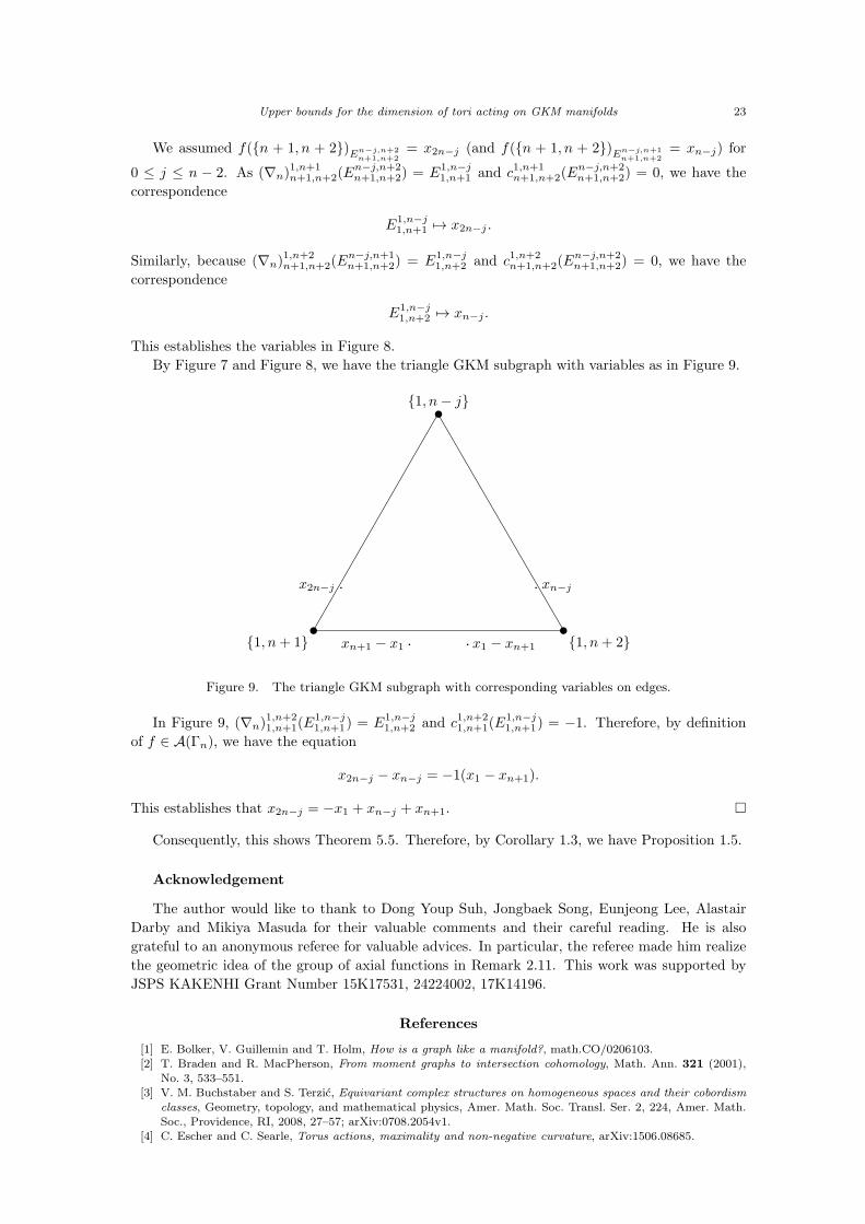
By Figure 7 and Figure 8, we have the triangle GKM subgraph with variables as in Figure 9.

{1, n− j}

{1, n+ 1} {1, n+ 2}

x2n−j xn−j

x1 − xn+1xn+1 − x1

Figure 9. The triangle GKM subgraph with corresponding variables on edges.

In Figure 9, (∇n)1,n+21,n+1(E

1,n−j1,n+1) = E1,n−j

1,n+2 and c1,n+21,n+1(E

1,n−j1,n+1) = −1. Therefore, by definition

of f ∈ A(Γn), we have the equation

x2n−j − xn−j = −1(x1 − xn+1).

This establishes that x2n−j = −x1 + xn−j + xn+1. □

Consequently, this shows Theorem 5.5. Therefore, by Corollary 1.3, we have Proposition 1.5.

Acknowledgement

The author would like to thank to Dong Youp Suh, Jongbaek Song, Eunjeong Lee, Alastair

Darby and Mikiya Masuda for their valuable comments and their careful reading. He is also

grateful to an anonymous referee for valuable advices. In particular, the referee made him realize

the geometric idea of the group of axial functions in Remark 2.11. This work was supported by

JSPS KAKENHI Grant Number 15K17531, 24224002, 17K14196.

References

[1] E. Bolker, V. Guillemin and T. Holm, How is a graph like a manifold?, math.CO/0206103.[2] T. Braden and R. MacPherson, From moment graphs to intersection cohomology, Math. Ann. 321 (2001),

No. 3, 533–551.[3] V. M. Buchstaber and S. Terzic, Equivariant complex structures on homogeneous spaces and their cobordism

classes, Geometry, topology, and mathematical physics, Amer. Math. Soc. Transl. Ser. 2, 224, Amer. Math.Soc., Providence, RI, 2008, 27–57; arXiv:0708.2054v1.

[4] C. Escher and C. Searle, Torus actions, maximality and non-negative curvature, arXiv:1506.08685.

24 S. Kuroki

[5] P. Fiebig, Moment graphs in representation theory and geometry, “Schubert calculus (Osaka 2012)” Adv. Stud-ies in Pure Math. 71 (2016), 75–96; arXiv:1308.2873.

[6] Y. Fukukawa, H. Ishida and M. Masuda, The cohomology ring of the GKM graph of a flag manifold of classical

type, Kyoto J. Math. 54, No. 3 (2014), 653-677.[7] O. Goertsches and M. Wiemeler, Positively curved GKM-manifolds, Int. Math. Res. Notices. (2015), 12015-

12041.[8] M. Goresky, R. Kottwitz and R. MacPherson, Equivariant cohomology, Koszul duality, and the localization

theorem, Invent. Math. 131 (1998), 25–83.[9] V. Guillemin, T. Holm and C. Zara, A GKM description of the equivariant cohomology ring of a homogeneous

space, J. Algebraic Combin. 23 (2006) no. 1, 21–41.[10] V. Guillemin, S. Sabatini and C. Zara, Balanced fiber bundles and GKM theory, Int. Math. Res. Not. IMNR

(2013), no. 17, 3886–3910.[11] V. Guillemin and C. Zara, One-skeleta, Betti numbers, and equivariant cohomology, Duke Math. J. 107, 2

(2001), 283–349.[12] W.Y. Hsiang, Cohomology theory of topological transformation groups. Ergebnisse der Mathematik und ihrer

Grenzgebiete, Band 85. Springer-Verlag, New York-Heidelberg, 1975.[13] S. Kuroki, Characterization of homogeneous torus manifolds, Osaka J. Math. 47 (2010), 285–299.[14] S. Kuroki, Classification of torus manifolds with codimension one extended actions, Transform. Groups 16

(2011), no. 2, 481–536.

[15] S. Kuroki, An Orlik-Raymond type classification of simply connected 6-dimensional torus manifolds withvanishing odd degree cohomology, Pacific J. of Math. 280-1 (2016), 89–114.

[16] S. Kuroki and M. Masuda, Root systems and symmetries of torus manifolds, Transform. Groups 22 (2017),

no. 2, 453–474.[17] H. Maeda, M. Masuda and T. Panov, Torus graphs and simplicial posets, Adv. Math. 212 (2007), 458–483.[18] J. W. Milnor and J. D. Stasheff, Characteristic Classes, Princeton Univ. Press, Princeton, N.J., 1974.[19] S. Takuma, Extendability of symplectic torus actions with isolated fixed points, RIMS Kokyuroku 1393 (2004),

72–78.[20] J. S. Tymoczko, Permutation actions on equivariant cohomology of flag varieties, Toric topology, 365–384,

Contemp. Math., 460, Amer. Math. Soc., Providence, RI, 2008.[21] T. Watabe, On the torus degree of symmetry of SU(3) and G2, Sci. Rep. Niigata Univ. Ser. A, 15 (1978),

43-50.[22] M. Wiemeler, Torus manifolds with non-abelian symmetries, Trans. Amer. Math. Soc. 364 (2012), no. 3,

1427–1487.[23] B. Wilking, Torus actions on manifolds of positive sectional curvature, Acta Math., 191 (2003), 259–297.

Shintaro Kuroki

Department of Applied Mathematics, Okayama University of Science, 1-1

Ridai-cho Kita-ku Okayama-shi Okayama 700-0005, JAPAN

E-mail: kuroki@xmath.ous.ac.jp