Alma Mater Studiorum · Universita di Bologna

FACOLTA DI SCIENZE MATEMATICHE, FISICHE E NATURALI

Corso di Laurea Specialistica in Fisica

Dynamical aspects of optical acceleration

and transport of protons

Tesi di Laurea in Meccanica Analitica

Relatore:Chiar.mo Prof.Giorgio Turchetti

Candidato:Stefano Sinigardi

II SessioneAnno Accademico 2009-2010

Sommario

Il lavoro di tesi, svolto nel gruppo V dell’INFN di Bologna, mi ha permesso di iniziare aconoscere un ambito di ricerca particolarmente attivo a livello internazionale. L’accelerazionedi particelle con l’uso di laser è diventato di notevole interesse grazie al rapidissimo aumentodi potenza che ha caratterizzato lo sviluppo dei laser nell’ultimo decennio.

L’accelerazione di elettroni ha già raggiunto un buon grado di comprensione teorica edi affidabilità sperimentale, grazie allo studio dei wake-fields. Le energie raggiunte sonodell’ordine dei GeV con apparecchi di dimensioni table-top e la qualità del fascio è tale chesono già allo studio sistemi multi-stage per acceleratori di particelle futuri.

Le tecniche di accelerazione laser-plasma sono invece ancora ampiamente sotto indagineper i protoni e gli ioni in generale. Solo recentemente si stanno iniziando ad avere risultatiinteressanti, con pacchetti di protoni di qualche MeV di energia. Grazie allo studio dinuovi bersagli gassosi, sembra possibile in un prossimo futuro ottenere protoni con energiedell’ordine del centinaio di MeV, sufficienti per avere interessanti applicazioni soprattutto inambito medico con l’adroterapia.

Nel primo capitolo di questa tesi descrivo le principali tecniche di accelerazione di ioniindagate fino ad oggi e i risultati che stanno mostrando. Quindi, nel secondo capitolo,analizzo metodi di simulazione computazionale del comportamento di un plasma e di unfascio accelerato, partendo dallo studio di diversi tipi di integratori numerici delle equazionidifferenziali che caratterizzano la meccanica del sistema, fino a giungere, nel terzo capitolo,alla modellizzazione degli elementi magnetici di una beamline che ne permetta il trasporto.

L’obiettivo è quello di iniziare la ricerca per l’ottimizzazione dei bersagli del laser, tramitel’identificazione di parametri minimi da soddisfare, e dei sistemi di trasporto, così che siapossibile un interfacciamento con apparecchi di post-accelerazione studiati da altri ricercatori

I

in contatto col nostro gruppo.

Per raggiungere questo obiettivo ho studiato diverse linee di trasporto, collaborando conil gruppo del Prof. Ratzinger dell’Università di Francoforte sul Meno (Germania) e conaltri ricercatori del GSI di Darmstadt (Germania). I risultati sono ancora preliminari mavengono qui presentati i più interessanti raggiunti durante il periodo di ricerca.

II

Introduction

In this thesis I will describe the work that I did with the 5th group of INFN in Bologna.The research field they’re working on is particularly active in Italy and in many othercountries.

Particle acceleration through laser has become really attractive in the latest years mainlythanks to the great power enhances that the lasers experienced recently. Electron accelera-tion with laser is known relatively well: many articles describe the laser wake field and theability of electrons to “surf” a magnetic wave to get energy. We already reach GeV energywith table-top devices and the beam quality is good enough that many multi-stage systemsare under development for future electron accelerators.

On the other hand, laser-plasma acceleration techniques are still under heavy investiga-tion for protons and ions in general. Only recently we’re starting to get interesting results,obtaining some bunches with few-MeV protons. Now, thanks to gaseous jet targets, it seemsthat in the near future we will be able to get protons with energies in the hundredth of MeV,enough to have some interesting applications in medical treatments (hadron-therapy)

In this thesis I will describe, in the first chapter, the main techniques known up todate to accelerate ions with lasers and their results. In the second chapter I will analysedifferent kinds of numerical integration techniques through a software that I wrote. Thoseintegrators are used to integrate the differential equations that describe the plasma motionand behaviour.

In the third chapter I will study the problems of transport of these bunches obtained fromlaser pulses. The goal is to optimize targets, through finding minimal necessary conditionsrequired on the initial distributions, and to study transport systems required to collect asmany protons as possible and bring them away from the interaction point. For the future,

III

we’re also considering matching the laser accelerated protons with a second-stage acceleratorand so we will need to design the best beamline.

To this aim, I studied and simulated with another software many different transportlines. I went also in Frankfurt am Main to work with Prof. Ratzinger’s group, to checkmy software results and to investigate, with other people from GSI (Darmstadt), differentsolutions for this problem. In this thesis I will describe the best results that I got duringthis research period.

IV

Contents

Sommario I

Introduction III

1 Laser-Plasma accelerators 1

1.1 What is a plasma? . . . . . . . . . . . . . . . . . . . . . . . . . . . . . . . . . 1

1.2 Particle acceleration . . . . . . . . . . . . . . . . . . . . . . . . . . . . . . . . 1

1.2.1 Accelerator basics . . . . . . . . . . . . . . . . . . . . . . . . . . . . . 2

1.3 Lasers . . . . . . . . . . . . . . . . . . . . . . . . . . . . . . . . . . . . . . . . 3

1.3.1 Chirped Pulse Amplification . . . . . . . . . . . . . . . . . . . . . . . . 3

1.4 Plasma physics . . . . . . . . . . . . . . . . . . . . . . . . . . . . . . . . . . . 3

1.4.1 Plasma accelerators . . . . . . . . . . . . . . . . . . . . . . . . . . . . 3

1.4.2 Characteristics of plasma . . . . . . . . . . . . . . . . . . . . . . . . . 6

1.4.3 Debye length . . . . . . . . . . . . . . . . . . . . . . . . . . . . . . . . 7

1.4.4 Plasma waves . . . . . . . . . . . . . . . . . . . . . . . . . . . . . . . . 9

1.4.5 Refraction index . . . . . . . . . . . . . . . . . . . . . . . . . . . . . . 10

1.4.6 Critical density and skin depth . . . . . . . . . . . . . . . . . . . . . . 11

V

1.5 Protons acceleration . . . . . . . . . . . . . . . . . . . . . . . . . . . . . . . . 12

1.5.1 Target Normal Sheath Acceleration . . . . . . . . . . . . . . . . . . . . 13

1.5.2 Radiation Pressure Acceleration . . . . . . . . . . . . . . . . . . . . . . 16

2 Integrators 29

2.1 Runge Kutta schemes . . . . . . . . . . . . . . . . . . . . . . . . . . . . . . . 32

2.1.1 Third order scheme (error order: τ4) . . . . . . . . . . . . . . . . . . . 35

2.1.2 Fourth order scheme (RK4 - error order: τ5) . . . . . . . . . . . . . . 35

2.2 Symplectic schemes . . . . . . . . . . . . . . . . . . . . . . . . . . . . . . . . . 35

2.2.1 First order symplectic integrators . . . . . . . . . . . . . . . . . . . . . 39

2.2.2 Second order symplectic integrators . . . . . . . . . . . . . . . . . . . . 41

2.3 Leapfrog integrators . . . . . . . . . . . . . . . . . . . . . . . . . . . . . . . . 42

2.3.1 Second order scheme (LF2) . . . . . . . . . . . . . . . . . . . . . . . . 43

2.3.2 Fourth order scheme (LF4) . . . . . . . . . . . . . . . . . . . . . . . . 46

2.4 PICcol: my code to compare integrators in a PIC environment . . . . . . . . 47

3 Protons transport 51

3.1 Transport of protons coming from TNSA regime . . . . . . . . . . . . . . . . 52

3.2 Lilia and Prometheus . . . . . . . . . . . . . . . . . . . . . . . . . . . . . . . . 53

3.3 My experience at the Goethe University in Frankfurt . . . . . . . . . . . . . . 54

3.3.1 BuGe: my bunch generator . . . . . . . . . . . . . . . . . . . . . . . . 55

3.4 Propaga . . . . . . . . . . . . . . . . . . . . . . . . . . . . . . . . . . . . . . . 59

3.4.1 Introduction to our code . . . . . . . . . . . . . . . . . . . . . . . . . . 59

3.4.2 Maps of the beamline elements . . . . . . . . . . . . . . . . . . . . . . 60

3.5 Our simulations . . . . . . . . . . . . . . . . . . . . . . . . . . . . . . . . . . . 66

3.5.1 Bunches from PIC simulations . . . . . . . . . . . . . . . . . . . . . . 66

3.5.2 The typical beamlines analysed . . . . . . . . . . . . . . . . . . . . . . 67

3.5.3 Status of the code at the end of the Frankfurt period . . . . . . . . . . 70

3.5.4 Simulations with K-V bunches . . . . . . . . . . . . . . . . . . . . . . 70

VI

3.5.5 The hard edge approximation removed . . . . . . . . . . . . . . . . . . 73

3.5.6 Future work . . . . . . . . . . . . . . . . . . . . . . . . . . . . . . . . . 74

Conclusion 77

Bibliography 79

VII

VIII

CHAPTER 1

Laser-Plasma accelerators

1.1 What is a plasma?

A plasma is a ionized gas. We should know about three states of matter: solid, liquid andgas. When a solid is heated enough, the thermal motion of the atoms breaks the lattice thatbuilds the crystal and usually a liquid is formed. In the same way, a liquid heated over theboiling temperature has the property that its atoms vaporize faster than they re-condense.

Similarly, when a gas is heated sufficiently, collisions between atoms make them mislaytheir loosely bound electrons. The ions-electron mixture that we get is commonly called aplasma [1].

1.2 Particle acceleration

Particle acceleration is used as a way to answer profound questions about our universe.Giant machines accelerate those little fundamental elements of the matter to nearly the speedof light and then smash them together. In this way, it’s possible to recreate conditions thatexisted when our universe was born in the big bang and unleash all the possible particlesand interactions that exist, to understand how they are all connected, described and, maybe,unified in a single theory.

Unfortunately, to achieve always greater energies, we have to build bigger and more

1

expensive particle accelerators. The most powerful one at the moment is the LHC, madeby CERN in Geneva1. It has reached every possible limit of what is technologically andeconomically feasible. Will advances in the science and engineering of particle acceleratorsbe continuous so that we can have something else after LHC?

A new approach to particle acceleration, using the plasma state of matter, is showingconsiderable promise for realizing a new type of accelerators, dramatically reducing theirsize and cost.

This is only one part of the story: particle acceleration is also really important formaterial science, structural biology, fusion research, transmutation of nuclear waste andnuclear medicine, such as treatment of certain types of cancer, among others. Of course, inthese cases, smaller ordinary machines are used now, but they still occupy large laboratoryspaces. Plasma accelerators promise extremely compact devices even in this smaller energyrange [2].

1.2.1 Accelerator basics

Accelerators propel either lighter particles (such as electrons and their antiparticle,positrons) or also heavier ones (protons, anti-protons and ions).

They can boost particles in a single passage (linear accelerators) or in many orbits (circu-lar ring accelerators). A big problem of non linear acceleration is a process called synchrotronradiation. As we will see, linear acceleration (preferably of electrons and positrons) is whatplasma based accelerators are most suited for.

A conventional linear collider accelerates its particles with an electric field that movesalong in synchrony with the particles. A structure called a slow-wave cavity (a metallicpipe with periodically placed irises) generates the electric field using powerful microwaveradiation. The use of a metallic structure limits how large the accelerating field can be. Ata field of 20-50 MV/m, electrical breakdown occurs — sparks jump and current dischargesfrom the walls of the cavities.

Because the electric field has to be weaker than the threshold for breakdown, it takes alonger acceleration path to achieve a specific energy. For example, a TeV beam would requirean accelerator 30 kilometers long. If we could accelerate particles far more quickly than isallowed by the electrical breakdown limit, the accelerator could be made more compact.That is where plasma comes in.

1http://lhc.web.cern.ch/lhc/ contains a lot of info about the Large Hadron Collider and its scientificprogram.

2

1.3 Lasers

In the last twenty years, the maximum power of the lasers has increased many order ofmagnitude, reaching intensities over 1021 W/cm2. The field, at these values, reaches 1012

V/m, so it’s greater than the electric field that binds electrons to the nucleus.

Electrons knocked by these intense electromagnetic pulses oscillate at relativistic speeds,with pulses up to 10 MeV/c. Radiation pressure made by laser is extreme and easily reachesterabars: we will describe it in the next chapter 1.5.

When a so strong pulse interacts with matter, it instantly ionizes everything, creating aplasma.

1.3.1 Chirped Pulse Amplification

The power increased so much in these years thanks to the Chirped Pulse Amplification(CPA) technique [3]. The fundamental idea is to use three devices: a “stretcher” and a“compressor”, with an amplification crystal. We use a first pulse, made by a low power laser(oscillator) which is able to create a really short packet, ∼ 10 fs, then we “stretch” it to∼ 10 ns. Then the pulse is amplified by the crystal, pumped by another laser, to get anamplification of 10 order of magnitude (so that we get an energy of a Joule). The pulse isthen “compressed” back to the oscillator length.

The transverse dimensions of these pulses are approximately between some centimetersup to a meter. The reason is that the great electric fields intensities would ionize the airand could destroy everything. We have to focus them using a parabolic mirror to get peaksof 1021 W/cm2 [4].

1.4 Plasma physics

1.4.1 Plasma accelerators

In a plasma accelerator, the role of the accelerating structure is played by the plasma.Instead of being a problem, electrical breakdown is part of the design because the gas isalready broken down at the beginning. There’s virtually no theoretical limit to the fieldthat can be produced in a plasma, as long as quantum effects don’t need to be considered.The power source is not microwave radiation but is either a laser beam or a charged particlebeam.

At first sight, laser beams and charged particle beams do not seem well suited for particleacceleration. They can have very strong electric fields, but the fields are mostly perpendic-ular to the direction of propagation. To be effective, the electric field in an accelerator has

3

to point in the direction that the particle travels. Such a field is called a longitudinal field.Fortunately, when a laser or charged particle beam is sent through a plasma, interactionwith the plasma can create a longitudinal electric field.

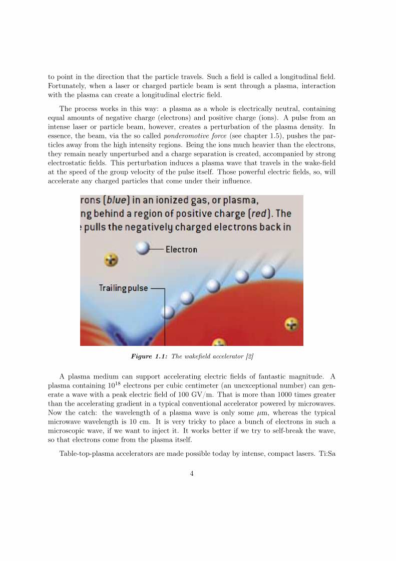
The process works in this way: a plasma as a whole is electrically neutral, containingequal amounts of negative charge (electrons) and positive charge (ions). A pulse from anintense laser or particle beam, however, creates a perturbation of the plasma density. Inessence, the beam, via the so called ponderomotive force (see chapter 1.5), pushes the par-ticles away from the high intensity regions. Being the ions much heavier than the electrons,they remain nearly unperturbed and a charge separation is created, accompanied by strongelectrostatic fields. This perturbation induces a plasma wave that travels in the wake-fieldat the speed of the group velocity of the pulse itself. Those powerful electric fields, so, willaccelerate any charged particles that come under their influence.

Figure 1.1: The wakefield accelerator [2]

A plasma medium can support accelerating electric fields of fantastic magnitude. Aplasma containing 1018 electrons per cubic centimeter (an unexceptional number) can gen-erate a wave with a peak electric field of 100 GV/m. That is more than 1000 times greaterthan the accelerating gradient in a typical conventional accelerator powered by microwaves.Now the catch: the wavelength of a plasma wave is only some µm, whereas the typicalmicrowave wavelength is 10 cm. It is very tricky to place a bunch of electrons in such amicroscopic wave, if we want to inject it. It works better if we try to self-break the wave,so that electrons come from the plasma itself.

Table-top-plasma accelerators are made possible today by intense, compact lasers. Ti:Sa

4

lasers that can generate 10 TW of power in ultra-short light pulses now fit on a large tabletop[5]. In a laser-powered plasma accelerator, for example, an ultra-short laser pulse is focusedinto a helium supersonic gas jet that can be some millimeters long. The pulse immediatelystrips off the electrons in the gas, producing a plasma. The radiation pressure of the laserbullet is so great that the much lighter electrons are blown outward in all directions, leavingbehind a positively charged region. These electrons cannot go very far, because the electricfield generated by the charge displacement pulls them back. When they reach the axisthe laser pulse is traveling along, another pulse overshoots them and they end up travelingoutward again, producing a wavelike oscillation [Figure 1.1]. The oscillation is called a laserwake-field because it trails the laser pulse like the wake produced by a motorboat.

Unfortunately, the accelerated electrons had a very wide range of energies — from 1 to200 MeV. Many applications require a beam of electrons that are all at the same energy.This energy spreading occurred because the electrons were trapped by the wake-field waveat various locations and at different times. In a conventional accelerator, particles to beaccelerated are injected into a single location near the peak of the electric field. Researchersthought that such precise injection was impossible in a laser wake-field accelerator becausethe accelerating structure is microscopic and short-lived.

The accelerated electron bunch can be externally injected, using a conventional acceler-ator, another laser-plasma stage or “internally” injected. This kind of injection comes fromthe so called wavebreaking of the plasma wave generated in the trail of the laser pulse. Inparticular conditions, the electron front at the peak density in the wake of the laser pulsecan break like a wave in the sea. When some of the electrons of the wave have a speed higherthan the wave velocity they leave the collective motion and find themselves injected in frontof the wave (a kind of foam, speaking in sea-terms!). An injected electron bunch experiencesthe strong accelerating electric field previously described and travels in the wake of the laserpulse gaining high energies. The most easily obtained wavebreaking comes spontaneouslywhen the density perturbation is very high.

Many techniques are already used or under development and they ensure a high mono-chromaticity of the electron bunches generated by a plasma accelerator and a small emit-tance. These techniques aim to induce the wave breaking in more controlled ways, forexample using a non uniform gas jet (the plasma wave speed depends on the plasma den-sity), or using a second weak counter-propagating laser which perturbs for a short time theplasma wave.

This small energy spread and the small emittance of the produced electron bunches,together with their very short time duration, might allow the development of multi-stagedplasma accelerators in the near future.

The laser-plasma interaction, using different experimental setups, can also be used toaccelerate heavier ions. Unfortunately, many of these techniques require that the injectedprotons/ions must be already traveling at nearly the speed of light, so they are not leftbehind by the plasma wave. For protons, that means an injection energy of several GeV.

5

Other alternatives, described in this thesis, use the strong electric fields that the chargedisplacement creates to accelerate ions (protons) up to some MeV. The protons/ions comefrom the target itself, often from a hydrogen-rich layer placed above it.

Physicists are making rapid progress in the quest for a plasma accelerator. Althoughmany of the fundamental physics issues are solved, the making of practical devices still posesformidable challenges. In particular, beam engineers must achieve adequate beam quality,efficiency (how much of the driver beam’s energy ends up in the accelerated particles),and alignment tolerances (the beams must be aligned to sub µm at the collision point).Finally, the repetition rate of the device (how many pulses can be accelerated each second)is important.

It took conventional accelerator builders 75 years to reach electron-positron collisionenergies in the range of 200 GeV. Plasma accelerators are progressing at a faster rate, andresearchers hope to provide the new technology to go beyond the microwave systems forhigh-energy physics in just a decade or two. Much sooner than that, the companion laserwake-field technology will result in GeV tabletop accelerators for a rich variety of applications[6].

1.4.2 Characteristics of plasma

Plasma is pervasive in nature: surfaces of stars, interstellar gases, Terrestrial magneto-sphere, these are all examples of plasmas.

The science of plasma physics was developed both to understand these natural phenom-ena and to explore the realm of controlled nuclear fusion.

What are the characteristics of plasmas? The important point is that the dynamics ofmotion are determined only by forces between near atoms of the material: the range of theforces in such a configuration is limited.

Let’s start with a system of N charges, which are coupled one to another via their self-consistent electric and magnetic fields. If we need to consider each and every aspect of thosecharges, we would have 6N coupled equations.

Fortunately, a very great simplification is possible if we focus our attention to collision-less plasma: in this case, we can decompose the electric field in two parts. E1 has a spacevariation on a scale thinner than the Debye length, which is the length over which the field ofan individual charge is shielded out by the surrounding particles, and represents the rapidlyfluctuating microfield. E2, on the other hand, represents the field due to deviations fromcharge neutrality over space scales greater than the Debye length [7].

6

1.4.3 Debye length

Let’s consider a uniform charge distribution, electrons for example, with density n0. Ina neutral plasma, we will have an equal distribution of ions, so that the system is neutral.Let’s suppose that some electrons get moved so that their density becomes n 6= n0, in away that we could write n = n0 + n1. The basic hypothesis that we do is that the newdistribution is in thermal equilibrium at a temperature T . Under these conditions, denotingthe potential generated by the n distribution with V , we have

n = n0 exp(eV/kBT )

where, as obvious, e is the electron charge. Defining with ρ = −en the charge density, wecan write the Poisson potential as

∇2V = −4πρ1 = 4πe n1 = 4πe n0 [exp(eV/kBT )− 1]

letting n1 = n− n0.

Defining

Φ =eV

kBT

we can write the Poisson potential in this way

∇2Φ = 4πe n0e

kBT[exp(Φ)− 1] (1.1)

Introducing the classical electron radius

rc =e2

mec2

equation 1.1 becomes

∇2Φ =4πrcn0mec

2

kBT= λ−2

D [exp(Φ)− 1] (1.2)

where we defined the Debye length as

λ2D =

1

4πrcn0

kBT

mec2(1.3)

In a one spatial dimensional world, eq. 1.2 can be integrated. In our 3-dimensionalworld, we can only obtain a solution spherically symmetric. Remembering that the radialpart of the Laplacian, in polar coordinates, is written as

∇2 = r−1 ∂2

∂r2r

7

and assuming r′ = r/λD, eq. 1.2 becomes

d2

dr′2(rΦ) = r′ [exp(Φ)− 1] (1.4)

For small charge imbalances, Φ 1, we have

d2

dr′2(r′Φ)− r′Φ = 0

and its solution is given by

Φ = Ce−r

′

r′V = Q

e−r/λD

r

in which Q is a constant. Let’s call q(r) the charge within a sphere of radius r and let’sapply the Gauss theorem to calculate it. We denote with S(r) a sphere of radius r centredin the origin of the axes and with Σ its surface. Then the charge contained within the spherecan be expressed by

q(r) =

∫S(r)

ρ(r′)dr =1

4π

∫S(r)

divE dr =1

4π

∫Σ(r)

E · rrdσ = r2Er(r)

In the case of a shielded potential, we have

Er(r) = −∂V∂r

= Qe−r/λD(

1

λDr+

1

r2

)We obtain q(0) = Q and so the charge density can be written as a regular part ρreg plus asingularity that corresponds to the point charge in the origin ρsing = Qδ(r).

ρ(r) = Qδ(r) + ρreg

We now write

q(r) = Q+ qreg(r) qreg(r) =

∫S(r)

ρreg(r′)dr

and, analogously,

Er(r) =Q

r2+ Ereg(r)

where it’s evident that the regular contribute of the charge density goes to zero when λD →∞.

So we getq(0) = Q q(∞) = 0

according to the fact that if we put a charge +Q in 0 we must also distribute an oppositecharge −Q in the whole surrounding space.

8

We now note that density ρ(r) is now defined by

ρ(r) = Qδ(r) + ρreg ρreg =q′(r)

4πr2= −Qe

−r/λD

4πλDr2

The contribution from the regular part is zero when λD → ∞. In this limit, only thesingularity given by the charge Q in the origin survives.

1.4.4 Plasma waves

When studying laser acceleration, we consider an adimensional parameter given by theratio between the rest electron energy and the electromagnetic field energy:

a =eA

mec2(1.5)

We can also define a similar ap in which the mass of the electron is replaced with the massof the proton.

An electromagnetic wave that propagates into a plasma excites density waves. We cansee that from these equations:

∂n

∂t+

∂

∂xi(vin) = 0

ρdvidt

= neEi

∂Ei∂xi

= 4πne

(1.6)

the first one is the continuity equation, the second one follows the conservation of linearmomentum and the third one is the Poisson’s equation; d

dt is the Eulerian derivative, so that

d

dt=

∂

∂t+∑k

vv∂

∂xk

Equilibrium requires that n = n0 and v = 0, E = 0. A disturbance in the density, measuredas n1, creates a field E1 and a drift v1 of the charged particles, so that now

n = n0 + n1 E ≡ E1 v ≡ v1

Keeping in mind that ρ = men the equations 1.6 become

∂n1

∂t+ n0

∂vi∂xi

= 0

medvidt

= eEi

∂Ei∂xi

= 4πn1e

(1.7)

9

Deriving the first equation by t and the second by xi, we get

∂2n1

∂t2= −n0

∂2vi∂t∂xi

= −n0e

me

∂Ei∂xi

(1.8)

The third equation of 1.6 becomes

∂2n1

∂t2+ ω2

pn1 = 0

in which

ω2p =

4πe2n0

me(1.9)

is the plasma frequency. Using the classical electron radius

re =e2

mec2= 3 · 10−13 cm

then 1.9 can be written asω2p = 4πrec

2n0 (1.10)

1.4.5 Refraction index

In linear approximation (electron density perturbations are small and so plasma oscilla-tions are harmonics of x2 potential type) we can note that the medium becomes opticallyactive and its refraction index can be calculated. Let’s consider fields in linear approxima-tion, too. So these equations are valid:

∇×B =4π

cj +

1

c

∂E

∂t

m∂v

∂t= eE

j = n0ev

(1.11)

We can choose periodic solutions

B = B∗e−iωt E = E∗e

−iωt D = D∗e−iωt v = v∗e

−iωt j = j∗e−iωt

so that

∇×B∗ =4π

c

n0e

m

E∗−iω

+−iωc

E∗ = −iωE∗(

1− 4πe2n0

mω2

)≡ −iωD∗

The Maxwell equation becomes

∇×B =1

c

∂D

∂tD = εE = n2

refrE

in which

nrefr =

(1−

ω2p

ω2

) 12

10

Dispersion relationships

The refraction index is given by the ratio between the group velocity and the vacuumlight speed

nrefr =vGc

(1.12)

from which we get, having said ω = ω(k) the dispersion relationship,

vG =dω

dk= cnrefr = c

(1−

ω2p

ω2

) 12

From here we obtain

kc =

∫ ω

ωp

ω′dω′(ω′2 − ω2

p

) 12

=1

2

∫ ω2

ω2p

dω′2(ω′2 − ω2

p

) 12

=(ω2 − ω2

p

) 12 (1.13)

andk2c2 = ω2 − ω2

p (1.14)

1.4.6 Critical density and skin depth

We note that if ω < ωp, the refraction index and the wave number turn into imaginary.There is no wave propagation any more, only a vanishing wave exponentially damped. For afixed frequency of the electromagnetic wave, the density for which we have ωp = ω is calledcritical density nc. For n > nc the plasma becomes opaque: the e.m. fields are dumped ona characteristic length `s.

The critical density is defined, using 1.10, by

ω2cr ≡ 4πrec

2ncr (1.15)

so that

ncr =ω2cr

4πc2re(1.16)

Using the known relation

λ =2π

k=

2πv

ω−→ λ2

cr =4π2c2

ω2cr

(1.17)

we get

ncr =π

λ2crre

=3.14

3× 10−1310−8λ2[µm]=

1021

λ2[µm]cm−3 (1.18)

11

If our density is above the critical one, n > ncr, we can define a skin depth as follows:

E = E0ei(kx−ωt) = e−iωte−x/`s (1.19)

in which `s = i/k.

Following from 1.14 we can write

k =1

c

(ω2 − ω2

cr

)1/2=

i

`s(1.20)

so that`s =

ic

(ω2 − ωcr)1/2=

c

(ωcr − ω2)1/2(1.21)

Using these results, we can write 1.21 as

`s =c(

ω2p − ω2

)1/2 =c

ω

(ω2p

ω2− 1

)−1/2

=λ

2π

(ω2p

ω2− 1

)−1/2

(1.22)

Calculating the ratio between ωp and ω using 1.10 and 1.15 we get that ω2p/ω

2 = ne/ncr

`s =λ

2π

(nencr− 1

)−1/2

If ωp ω, so that ne ncr, we have

`s ≈λ

2π

ncrne

=λω

2πωp=

c

ωp(1.23)

1.5 Protons acceleration

Acceleration of particles through laser pulses got a substantial progress in the last years,thanks to the dramatic increase of power obtained with the CPA (chirped pulse amplifica-tion). The protons and ions acceleration, after the first studies with the high energy Nd:glasslasers, has been developed using the low energy (but high power) Ti:Sa lasers [8].

The protons beam quality was initially very poor, but subsequent improvements (micro-structured targets, energy crossing the 10 MeV line) made possible to propose the use oflaser accelerated protons for therapy, even though many studies are still required before thelaser accelerated proton beams can be delivered to patients [9].

Recently, also CO2 lasers have been used: they have a very long wavelength, nativecircular polarization and a relatively good conversion efficiency. The problem with them is

12

their long pulse duration mixed with a low power, but both aspects are now finding newpeople willing to improve them thanks to recent interesting results [10].

There are two main laser regimes that produce protons acceleration: TNSA (TargetNormal Sheath Acceleration) and RPA (Radiation Pressure Acceleration).

1.5.1 Target Normal Sheath Acceleration

Most of the experiments about laser-plasma ion acceleration exploited this regime, focus-ing an intense laser pulse on a target with overcritical electron density (i.e. plasma formedby the ionization of a solid) with a high thickness (` > `s). Many experiments, also, considernon-normal incidence on the target foil.

The acceleration happens because electrons in the first layers get excited and becomehot for a thickness of a few `s. These electrons have an essentially diffusive motion, both inthe laser direction and in the opposite one.

The electrostatic field created by the charge imbalance accelerates the ions [11]. Beingthe diffusion quite isotropic, the accelerating fields experienced by the ions are strongest onthe surfaces of the foil and normal to them, on both sides of the target. We also get a lotof angular dispersion, with two main peaks on both rear and front direction along the laserbeam. The electrons cloud has a thickness of a few Debye lengths.

Let’s consider a pulse propagating along z axis, polarized along y. Conjugated momentaare:

Px = px Py = py −eAyc

= py −meca Pz = pz

Kinetic energy of an electron is given by:

T = mec2(γ − 1) = mec

2

[(1 +

p2

m2ec

2

)1/2

− 1

](1.24)

If A = Ay(z)ey were the vector potential of a fixed external field, then Py would beconserved exactly and would be zero because before the waves arrives we have Ay = py = 0.Because of the fluid nature of this problem, we can only say that Py = 0; coupled withpy = meca and pz = p, we can write the 1.24 as

T = mec2

[(1 +

p2

m2ec

2+ a2

)1/2

− 1

](1.25)

If no fields, other than those generated byA, are there, then the longitudinal accelerationis given by the ponderomotive force. Let’s see how a longitudinal force comes out: starting

13

from a quickly oscillating Ay(z), we can write

〈A(z, t)〉 = 0⟨A2(z, t)

⟩6= 0

Writing the LagrangianL =

me

2v2 +

e

cvy Ay(z)

we obtainPx = mex Py = mey +

e

cAy

The Hamiltonian is

H =1

2me

[P 2x +

(Py −

e

cAy

)2+ P 2

z

]=

=1

2me

[P 2x + P 2

y + P 2z − 2

e

cAyPy +

e2

c2A2y

](1.26)

x =Pxme

y =Pyme− e

mecAy z =

Pzme

z = Pz = −e2

c2

∂

∂z

⟨A2y

⟩(1.27)

The longitudinal motion is collective, while the transverse motion can be considered asthermal agitation (it will be suppressed in RPA regime as we will see).

Poisson-Boltzmann equation

The main role in the ion acceleration, so, is played by the hot electron component. Therelativistically strong laser pulse transfers its energy and momentum to electrons, that areaccelerated up to an energy of the order of magnitude of the laser ponderomotive potential.

The efficiency, ηe, of the energy conversion from laser to hot electrons should be of theorder of 20%-30%, but no real according exists in literature. After crossing the target, theelectrons distribute themselves over few Debye lengths λe,hot, which for ne,hot = 3 1019 cm−3

and Ee,hot = 6 MeV is λe,hot = 3 µm. But let’s consider this model in detail.

If we have a one dimensional slab along z, extending from z = 0 (the position of thesolid-vacuum interface at the rear side of the target before the arrival of the pulse) up tox = h (the farther limit of the electron cloud, that will be determined later), we couldassume that the hot electron density follows the Boltzmann distribution

ne(z) = n0 exp

[eV

kBT

](1.28)

14

where V = V (z) is the electrostatic potential, n0 is the value of the hot electron density atV = 0 and T is the constant temperature of the electrons produced by the laser pulse.

This is, of course, a simplification, as it would be better to use a more complicatedelectron distribution function [12].

By assuming that, over the electron time scale, the ion distribution remains localized(immobile ions), the Poisson-Boltzmann equation in the “vacuum” region, that is for z ≥ 0,reads

d2V

dz2= 4π e n0 exp(eV/kBT ) (1.29)

A problem arise, because the rhs of 1.28 does not vanish for z → +∞, unless V (+∞)→−∞. This situation is not acceptable, because any positively charged particle at z = 0would be accelerated indefinitely in such a potential distribution. We must introduce anupper boundary h, chosen on the basis of the electron energy conservation [13]: the kineticenergy acquired by a test electron from the laser pulse should be equal to the work donefrom the electron to cover the distance h in the presence of the spatial distribution of theother fast electrons. It results:

h =

√γe − 1

πrcnav

in which rc is the usual classical electron radius, γe is the relativistic factor of the testelectron and nav is the average density of hot electrons.

Equation 1.29, coupled with eq. 1.28, is then solved with boundary conditions V (h) = 0and V ′(h) = 0. These conditions mean that ne(h) = n0 and ne(z > h) = 0, so that there’sa discontinuity in the electron distribution at z = h. However, due to the other boundarycondition, the corresponding electric field profile is continuous, being zero at z = h.

Defining

Φ =eV

kBTζ =

z

λDη = h/λD (1.30)

and using kB = 1 going on, the equation 1.29 becomes

d2Φ

dζ2= eΦ (1.31)

To solve it, we must use, as we previously said, Φ(η) = Φ′(η) = 0. The prime integral ofthe motion, noting that the potential is −eΦ and so not forgetting conditions at ζ = η, is

1

2

(dΦ

dζ

)2

− eΦ = −1

so that√

2

∫ ζ

ηdζ ′ =

∫ Φ

0

dφ√eφ − 1

(1.32)

15

Using u = eφ we get√

2(ζ − η) = 2

∫ eφ

1

d√u− 1

u

Inserting now w =√u− 1

ζ − η√2

=

∫ √eφ−1

0

dw

1 + w2= arctan

√eφ − 1

Φ = log

(1 + tan2

(ζ − η√

2

))Going back to original quantities, using the 1.30 relations, we have

V (z) =T

elog

(1 + tan2

(h− zλD√

2

))

The electric field is

εz = −V ′(z) =T

e

√2

λDtan

h− zλD√

2

It’s now easy to get the maximum energy:

Emax = Ze V (0) = ZT log

(1 + tan2

(h

λD√

2

))(1.33)

Experimental results are different from these calculations: electrons energy depends notonly on laser intensity but also on its energy and duration. Passoni [14] developed a morerealistic model, with cold and hot electron populations, slow heavy ions and fast lighterones, to describe metals with a small hydrogen rich surface.

1.5.2 Radiation Pressure Acceleration

Radiation Pressure Acceleration (RPA) is a viable method to obtain ions up to energiesof some GeV/nucleon, and so up to the relativistic domain. It’s an alternative route to thebetter understood TNSA regime; it has been developed and stimulated by simulations ofEsirkepov et al. [15, 16], in which they show that at intensities I > 5 × 1021 W/cm2 RPAstarts to dominate over TNSA.

It’s a different mechanism, particularly enlightened with circularly polarized laser pulses:in such conditions, the acceleration of “fast” electrons at the laser–plasma interface is almostsuppressed, ruling out TNSA which is driven from the space charge produced by energetic

16

electrons escaping in vacuum. Electrons heating become negligible: it’s the ponderomotiveforce that acts directly accelerating electrons and ions in the RPA regime [17].

A simple minimal model to show the role of the polarization in laser interaction with anoverdense plasma can be described as follows: let’s assume a plane, elliptically (circularlyif ε = 1) polarized wave of frequency ω. It’s incident on an overdense plasma with astep–like profile of the electron density (ne(x) = n0 θ(x)). We assume ωp > ω, being ωp =√

4πn0e2/me the plasma frequency.

For sufficiently low intensity the vector potential inside the plasma can be written as

A(z, t) =A(0)√1 + ε2

e−z/`s (x cosωt+ εy sinωt) (1.34)

where `s = c/√ω2p − ω2 (1.22) and ε is the ellipticity (0 < ε < 1).

The longitudinal force on electrons due to the v×B term is then obtained, like in 1.27,as

Fz = − e2

2mec2∂zA

2 = F0e−2z/`s

(1 +

1− ε2

1 + ε2cos 2ωt

)So, from a microscopic point of view, Prad (radiation pressure) is given by the integral

of temporal average of the Lorentz’s law F = J × B over a period of the electromagneticfield and over the target volume. Since this ponderomotive force (its density is called fp)scales with the inverse of the particle mass, its effects on ions are negligible. In fact, thetransfer of momentum to ions is actually mediated by the electrostatic field generated bythe displacement of the electrons under the action of fp [18].

If fp and the electrostatic force on electrons coming from unmoved ions balance eachother, so that we can say that the electrons are in a mechanical equilibrium, the totalelectrostatic pressure Pes on ions is given by the integral of ZeniEes. If the condition ofquasi-neutrality Zeni = ene holds, then ZeniEes = eneEes = fp, yielding Pes = Prad. Inthese conditions one can effectively assume that the target ions are pushed by Prad

We have two models for this regime, depending on the thickness of the target: the HoleBoring (HB) model, for thicker targets, and the Light Sail (LS) model, for thinner ones.

Hole Boring Regime

The model is best described with the help of the figure 1.2. The first frame (a) cor-responds to the initial stage in which the electrons have piled up under the action of theradiation pressure, creating the space-charge field Ex, which balances the ponderomotiveforce. We can say that electrons are in equilibrium and ions did not move significantly. Sowe can describe Ex and ne with those simple profiles, that approximate the exact profilescalculated in steady conditions [19].

17

Figure 1.2: Profiles of the ion density ni (blue), electron density ne (green) andelectrostatic field Ex (red) at three different stages of ion acceleration [17].

Given the original expression by J. C. Maxwell

Prad = (1 +R)I

c(1.35)

the model parameters xd, E0 and np0 shown in 1.2 are related to each other by the Poissonequation, the law of charge conservation and the equilibrium condition.

Pes =

∫eneExdx

.= Prad = 2

I

c

when we assume total reflection (R = 1). The penetration distance of the ponderomotiveforce into the target is `s = xs − xd and is of the order of the collisionless skin depthdp = c/ωp (ωp is the plasma frequency). This simple profile allows us to solve motionequations analytically: we easily find that all ions in this region get to xs at the same time,with an energy spectrum that is a flat-top distribution extending from zero to the cut-offvalue of

Emax =mp

2v2m = 2mpc

2Π (1.36)

where

vmc

= 2Π1/2, Π =v2m

4c2, Π =

I

minic3=

(Z

A

)ncne

me

mpa2

0.

(a0 is the dimensionless pulse amplitude corresponding to the field intensity I (for circularpolarization), A is the atomic mass number).

What we observe from simulations is that the fastest ions form a narrow bunch of velocityvm that penetrated into the overdense plasma. The other ions form another peak movingwith a velocity vb = vm/2. Simply, we can say that vb is the speed at which a hole is boredinto the plasma.

18

In [20, 21, 22] they propose a relativistic variant of 1.36. The main point is the use ofmomentum conservation in the reference frame that is co-moving with the target surface.In this reference frame, the intensity is I ′ = I (1− vb/c) / (1 + vb/c) or, using β = vb/c,I ′ = I(1− β)/(1 + β).

Using this relation, they found this new form of the equation:

Emax = 2mpc2 Π

1 + 2Π1/2(1.37)

This means that the transfer of energy from EM wave to the plasma, in the laboratoryframe of reference, occurs because of the frequency redshift of each photon that is reflectedfrom the moving surface of the plasma. This energy is proportional to the relative shift, andlike the intensity we get ω′/ω = (1− vb/c) / (1 + vb/c).

The scaling of the ion energy with the laser intensity and the target density, which canbe derived from equations 1.36-1.37, is unfavourable if we aim at relativistic energies. Fortargets at solid densities, ne > 100nc, values of Π ≈ 1 cannot be approached even at thehighest intensities available for the next years. To obtain Π ≈ 10−1, that means ≈ 100 MeVper nucleon (useful in hadron-therapy), we must use targets with density of only a few nc.

To produce ions with energy exceeding 102 MeV we must wait for technologies like thefew-cycle pulses at ultrahigh intensity.

Light Sail regime

The model of this regime is based on the concept of a totally reflecting plane mirrorboosted by a light wave. For long enough values of pulse duration τL, such that vbτL > `,being ` the thickness of the target, the hole boring through the target is “complete” andall the ions are displaced by the radiation pressure. For a very thin target having ` ≤ `s(`s is the penetration distance of the ponderomotive force into the target) all the ions areaccelerated as a single bunch. The average motion of the target can be described as that ofa reflecting object boosted by the radiation pressure.

Let’s consider a mirror that is moving along the positive direction of the x axis withspeed u with respect to the lab frame of reference S. We denote with xµ the contravariantcoordinates in S and x′µ those in S′ co-moving with the mirror.

So we can write:

x0 = ct, x1 = x, x2 = y, x3 = z.∂x′α

∂xβ= Lαβ

19

Our convention is to use a Minkowsky metric like the following:

gαβ =

1 0 0 00 −1 0 00 0 −1 00 0 0 −1

We denote with x the vector column made by the xµ and with xµ the covariant compo-

nents. The relation between them is this:

xµ = gµνxν xµ = gµνxν gµαgαν = δµν

For the Minkowsky metric tensor we have gµν = gµν . The relativistic invariance x′µx′µ =xµxµ can be written as

x′µgµνx′ν = xµgµνx

ν −→ x′ = Lx

x′ · gx′ ≡ Lx · gLx = x · LgLx

(L is the transpose) so that the invariance implies LgL = g.

Remembering that

β =u

cγ =

(1− β2

)−1/2

we can write the matrix for the Lorentz transformation along the x axis as

L =

γ −βγ 0 0−βγ γ 0 0

0 0 1 00 0 0 1

It’s easy to note that

• LgL = g

• L = L

• detL = 1

• L−1(β) = L(−β)

20

Let’s compose two Lorentz transformations of this type:

L(β1) =

γ1 −β1γ1 0 0−β1γ1 γ1 0 0

0 0 1 00 0 0 1

L(β2) =

γ2 −β2γ2 0 0−β2γ2 γ2 0 0

0 0 1 00 0 0 1

L(β1) · L(β2) =

γ1γ2 + β1β2γ1γ2 −β2γ2γ1 − β1γ1γ2 0 0−β1γ1γ2 − β2γ1γ2 β1γ1β2γ2 + γ1γ2 0 0

0 0 1 00 0 0 1

If we limit ourselves to consider the first matrix block 2× 2, we can rewrite the Lorentz

composition in this way:

L(β1) · L(β2) = γ1γ2

(1 + β1β2 −β1 − β2

−β1 − β2 1 + β1β2

)

Using

β =β1 + β2

1 + β1β2=u

c

in whichu =

u1 + u2

1 + u1u2/c2

we can rewrite the composition in this really simple way:

L(β) = L(β1) · L(β2) = γ

(1 −β−β 1

)in which γ, thanks to the fact that detL(β) = 1 = detL(β1) · detL(β2), has the usualdefinition

γ =1√

1− β2=

1 + β1β2

γ1γ2

Let’s write the usual electromagnetic field tensor

Fµν = ∂µAν − ∂νAµ =

0 −Ex −Ey −EzEx 0 Bz ByEy −Bz 0 BxEz By −Bx 0

21

As we know, it’s defined so that Fµν = −Fνµ

If we consider the Lorentz transformation of Fµν we find that

F ′µν = Lµα(−β)Lνβ(−β)Fαβ = Lµα(−β)FαβLβν(−β)

where we must note that the last term is equal to Lνβ thanks to L properties.

F ′ = L(−β)FL(−β)

F = L−1(−β)F ′L−1(−β) = L(β)F ′L(β)

If we impose that the mirror and the wave move both in the x > 0 verse, such that β ispositive (remember that the motion is only in the x direction), we find that the electromag-netic field tensor transforms itself in this way:

E′x = ExE′y = γ(Ey − βBz)E′z = γ(Ez + βBy)

B′x = BxB′y = γ(By + βEz)

B′z = γ(Bz − βEy)

Analysing a wave linearly polarized that propagates along the x direction we must setEx = Ez = 0Bx = By = 0

Ey = E0ei(kx−ωt)

Bz = B0ei(kx−ωt)

Remember the Maxwell’s equation (in the vacuum)

∇ ·E =ρ

ε0

∇×E = −∂B∂t

∇ ·B = 0

∇×B =1

c2

∂E

∂t

n.b.: we could also use the following conventions:rotE = −1

c

∂B

∂t−→ ∂Bz

∂t= −c∂Ey

∂x

rotB =1

c

∂E

∂t−→ ∂Ey

∂t= −c∂Bz

∂x

Substituting the plain wave expression, in which k = ω/c, we find that E0 = B0 and so

Ey = Bz

22

The Poynting vector isE×B = exEyBz = exE

2y

and it aims to the positive direction of the x axis.

We have found thatE′x = 0E′y = Ey(1− β)γ

E′z = 0

B′x = 0B′y = 0

B′z = Ey(1− β)γ

Wave intensity is derived from the modulus of the Poynting vector

I = EyBz = E2y I ′ = E′yB

′z = E′2y

so that we can writeI ′ = Iγ2(1− β)2 = I

1− β1 + β

which is consistent with the fact that wave intensity on the mirror decreases if it’s moving inthe wave direction and verse. I represents the energy flux (in W/m2) of an electromagneticfield. I divided by the square of the speed of light in free space is the density of the linearmomentum of the electromagnetic field. The time-averaged intensity 〈I〉 divided by thespeed of light in free space is the radiation pressure exerted by an electromagnetic wave onthe surface of a target; the transferred momentum is exactly its double, 2I/c. So we canwrite:

dP

dt= F ′x =

2I ′

c=

2I

c

1− β1 + β

in which F ′x is the force per unit of surface.

Denoting with µ the mass per unit of surface, we can write

µd

dt

u√1− u2/c2︸ ︷︷ ︸

acceleration

=2I

c

1− β1 + β

if we divide by µ c both sides we get:

d

dt

β√1− β2

=2I

µc2

1− β1 + β

If we use a wave packet instead of a plain wave we must write Ey = Ey(x− ct) =

∫f(k)eik(x−ct)dk

Bz = Ey

23

and we get the very well known equation for the relativistic mirror (or light sail):dw

dt=

√1 + w2 − w√1 + w2 + w

2

µcI(x− ct)

dx

dt= c

w√1 + w2

Choosing β as the independent value we getdβ

dt=

2

µcI(x− ct) · (1− β)2(1− β2)

1/2

dx

dt= cβ

The efficiency is measured in the case of a plane wave as a Doppler effect

wout

win=

(1− β1 + β

)1/2

Being hw the photon energy coming in and out, we finally get

η = 1− Elaser-out

Elaser-in= 1−

(1− β1 + β

)1/2

The mirror problem

The radiation pressure on a thin target in its rest frame, neglecting absorption and atnormal incidence, as we saw, is given by

Pthin = 2RthinI

c(1.38)

where Rthin is the reflectivity of the thin target.

Equation 1.38 is different from the original one for thick target 1.35 because we mustconsider now the transmitted wave.

The equation for the mirror is given by [23]dβ

dt=

2I0

µcf

(t− x/cτlaser

− 1

)1− β1 + β

(1− β2)3/2

dx

dt= cβ

(1.39)

in which µ is the superficial density and f describes the pulse I0 amplitude, in the interval0 ≤ t− x/c ≤ 2τlaser

24

We define the laser energy Elaser in this way, supposing that S is the surface enlightenedby the laser (spatially uniform):

Elaser = I0S

∫ (x/c)+2τlaser

x/cf(t)dt = I0SτlaserF (1.40)

in which F is the fluence (flux integrated over time):

F =

∫ 1

−1f(u)du (1.41)

For example, we can see that choosing a pulse like

f(ω) =

cos2 π

2ω |ω| < 1

0 |ω| ≥ 1

we have F = 1.

Let’s enter adimensional variables:

t′ =t

τlaserx′ =

x

cτlaser

Using the notation

λ =τlaserτ

τ =µc2

2I0

the equation 1.39 becomesdβ

dt′= λf

(t′ − x′ − 1

) 1− β1 + β

(1− β2)3/2

dx′

dt′= β

(1.42)

We now choose w = t′ − x′ − 1 and we find that f doesn’t change when w is between −1and 1. So we get:

dβ

dt′= λf(w)

1− β1 + β

(1− β2)3/2

dw

dt′= 1− β

(1.43)

We search the prime integral using the following method:

dH = C

[(1− β)dβ − λf(ω)

1− β1 + β

(1− β2

)3/2dω

](1.44)

If we chooseC = (1 + β) (1− β)−1(1− β2

)−3/2 (1.45)

25

putting 1.45 in 1.44, ω → ω′ and β → β′, we get

dH = λf(ω′)dω′ − 1 + β′

(1− β′2)3/2dβ′ (1.46)

Integrating from ω = −1 to ω and from β = 0 to β we get

H = λ

∫ ω

−1f(ω′)dω′ −

(1 + β

1− β

)1/2

(1.47)

Note that t = 0 means x = 0 and β = 0. Those become ω = −1 and β = 0 for t′ = 0 inthese gauge reduction, so that H = −1.

If we proceed through the end of the pulse, where ω = 1 and the speed is at its maximumβ∗, we find that

λF −(

1 + β∗1− β∗

)1/2

= −1 −→ β∗ =1 + λF 2 − 1

1 + λF 2 + 1(1.48)

Let’s define α as

α = λF =2I0τlaserF

µc2=

2I0SτlaserF

µSc2=

2Elaser

Emirror@rest(1.49)

Putting 1.49 in 1.48 we find

γ∗ − 1 =α2

2 + 2α(1.50)

Knowing that the kinetic energy of an ion of atomic mass A is

T = Ampc2(γ − 1)

we get

Tion = Ampc2(γ∗ − 1) = Ampc

2 α2

2 + 2α(1.51)

The kinetic energy of the enlightened mirror surface S, whose rest energy is Emirror@rest =µSc2, is

Tmirror = Emirror@rest(γ∗ − 1) = Emirror@restα

2

α

1 + α= Elaser

α

1 + α(1.52)

The result would have been the same using Tmirror = Tion ·Nions, where Nions = µS/(Amp).The efficiency of this regime is

η =Tmirror

Elaser=

α

1 + α(1.53)

26

As we can see, reducing the thickness enhances the efficiency and the ion’s energy in-creases as α. On the other hand, there’s an upper limit to the thickness of the target, overthat it becomes transparent. The mirror is opaque as long as

a < ζ = πnenc

`

λ

The number of protons (A = 1) that are into a cylinder with a base diameter S is

Nions = neS` =nencS`

π

rcλ2= ζ

S

λrc

To avoid transparency we need that

Nions ≥ N∗ions =S

λrca

The minimum thickness, so, is

`∗ =N∗ionsneS

=a

neλrc

27

28

CHAPTER 2

Integrators

We will analyse, in this chapter, the most important methods to solve ordinary differ-ential equations (ODEs) that describe the evolution of a system. We will limit ourselves tothe 2D case: (x, t).

Euler’s method

If we need to solve a differential equation like x = f(x, t), we can see how, on the righthand side, we have the definition for each and every point (x, t) ∈ D of the tangent curveto the solution x(t).

Let’s illustrate it better: we need to fix an arbitrary integration step τ , reasonablysmall. After the choice of an initial point (t0, x0) we calculate the approximate solution fort1 = t0 + τ calculating x(t1) = x(t0) + τf(x0, t0).

At this point, we know the value (t1, x1): we only have to repeat this cycle as long asit’s needed.

Of course, we do not have to forget that points calculated are only approximated and thereliability of the method depends on the chosen step and on the error propagation duringthe cycle. To evaluate better the error we are making, we can analyse the Taylor series andestimate the error at each time step:

x(t+ τ) = x(t) + τ x(t) +O(τ2)

29

Figure 2.1: Euler’s integration method: we approximate the curve with straightlines, adding a fixed quantity τ to t at each step

Each and every time step we are neglecting a remainder O(τ2).

Note: to use the Taylor expansion, we need that x(t) belongs to C1 class for its argu-ments, because we’re requiring that x(t) can be derived two times.

But how could I use this value to obtain the global error that I’m doing? It seems thatwe do not have any hint on this.

Let’s obtain the effective error done in many steps:

• k-order error [24]:

ek ≤ (∆t)mM

L

[eLtk − 1

]• Symplectic algorithm: no [24].

Let’s design a program1, using Wolfram Mathematica, that generate a numerical solutionto a first order initial value problem of the form

y′ = f(x, y) y(x0) = y0

using Euler’s method.

euler[f_, x_, x0_, xn_, y_, y0_, steps_] :=Block [xold = x0,1http://calculuslab.deltacollege.edu/ODE/7-C-1/7-C-1-b-ma.html

30

yold = y0,sollist = x0, y0,x,y,h

,h = N[(xn - x0)/steps];Do[xnew = xold + h;ynew = yold + h*(f /. x -> xold, y -> yold);sollist = Append[sollist, xnew, ynew];xold = xnew;yold = ynew,steps

];Return[sollist]]

We can try this simple code launching this command, for example:

soluzione1=euler[x+2y, x,0,1,y,0,40]

To enhance the graphical output we can use:

MatrixForm[soluzione1]

to obtain a table (matrix) form that is simpler to read, or:

ListPlot[soluzione1]

to obtain a graph with the points, or:

ListLinePlot[soluzione1]

to get an interpolation of the points and maybe the best possible output.

The parameters are:

• f , for the first order differential equation (in the example the equation is y′ = x+ 2y);

• x0, for the initial x value (x0);

31

• y0, for the initial y value (y0);

• xn, for the final x value;

• steps, for the number of subdivisions.

The key algorithm consists in finding new x and y values from the previous ones using

xn+1 = xn + h yn+1 = yn + hf(xn, yn)

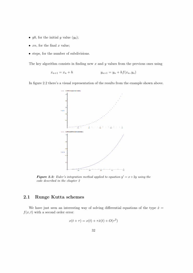
In figure 2.2 there’s a visual representation of the results from the example shown above.

Figure 2.2: Euler’s integration method applied to equation y′ = x+ 2y using thecode described in the chapter 2

2.1 Runge Kutta schemes

We have just seen an interesting way of solving differential equations of the type x =f(x, t) with a second order error:

x(t+ τ) = x(t) + τ x(t) +O(τ2)

32

We could try to enhance the precision of the algorithm including third order corrections: forexample

x(t+ τ) = x(t) + τ x(t) +τ2

2x+O(τ3)

But, beyond becoming more strict on requests to our function (it must belong to smootherclasses of functions), this method can be really tedious, making everything not feasible. Toimprove the precision without making more complex numerical and analytical calculations,our calculations can use Runge-Kutta methods. The fundamental idea is to calculate thestep between x(t) and x(t+ τ) using the first derivative in a middle point of the interval.

Let’s consider a generic function φ(t). We can see that:

φ(t+ τ) = φ(t+

τ

2

)+τ

2φ(t+

τ

2

)+

τ2

4 · 2!φ(t+

τ

2

)+O(τ3)

φ(t) = φ(t+

τ

2

)− τ

2φ(t+

τ

2

)+

τ2

4 · 2!φ(t+

τ

2

)+O(τ3)

Subtracting both on the lhs and on the rhs we get

φ(t+ τ)− φ(t) = τ φ(t+

τ

2

)+O(τ3)

The error is a third order one, even if the final calculation only uses first derivative. Thishappened because subtracting we cancelled the term φ. Summing, on the other hand (orbetter, on both hand sides!), we get:

φ(t+

τ

2

)=φ(t) + φ(t+ τ)

2+O(τ2)

Also in this case the term φ is lost and we get an order of precision in τ .

There exist many Runge-Kutta methods. Let’s look a first one.

Let’s replace x(t) to φ(t) in the subtraction previously done. Remembering that we wantto solve the equation x = f(x, t), we get the solution

x(t+ τ)− x(t) = τf(x(t+

τ

2

), t+ τ/2

)(2.1)

It’s not useful as a solution because it depends on x(t+ τ/2) which is unknown; we stillcan approximate it with the Euler’s method previously seen, so that

x(t+ τ/2) = x(t) +τ

2f (x(t), t) +O(τ2)

as can be seen from figure 2.3

33

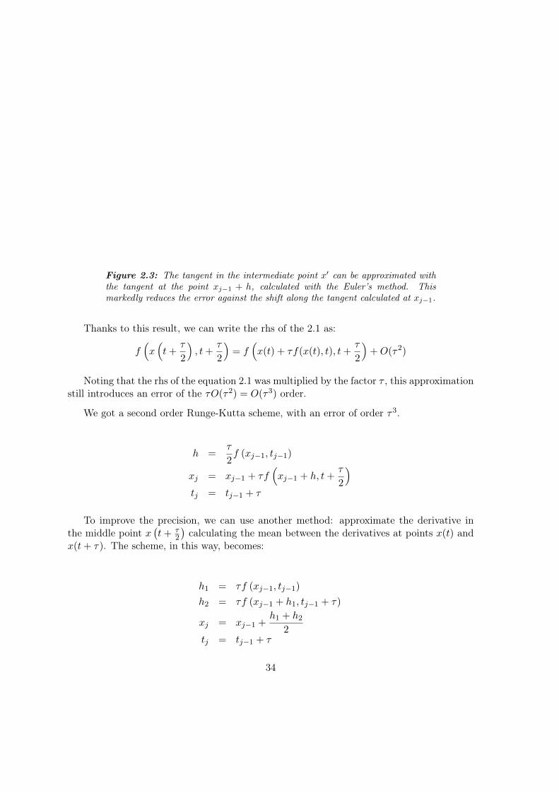
Figure 2.3: The tangent in the intermediate point x′ can be approximated withthe tangent at the point xj−1 + h, calculated with the Euler’s method. Thismarkedly reduces the error against the shift along the tangent calculated at xj−1.

Thanks to this result, we can write the rhs of the 2.1 as:

f(x(t+

τ

2

), t+

τ

2

)= f

(x(t) + τf(x(t), t), t+

τ

2

)+O(τ2)

Noting that the rhs of the equation 2.1 was multiplied by the factor τ , this approximationstill introduces an error of the τO(τ2) = O(τ3) order.

We got a second order Runge-Kutta scheme, with an error of order τ3.

h =τ

2f (xj−1, tj−1)

xj = xj−1 + τf(xj−1 + h, t+

τ

2

)tj = tj−1 + τ

To improve the precision, we can use another method: approximate the derivative inthe middle point x

(t+ τ

2

)calculating the mean between the derivatives at points x(t) and

x(t+ τ). The scheme, in this way, becomes:

h1 = τf (xj−1, tj−1)

h2 = τf (xj−1 + h1, tj−1 + τ)

xj = xj−1 +h1 + h2

2tj = tj−1 + τ

34

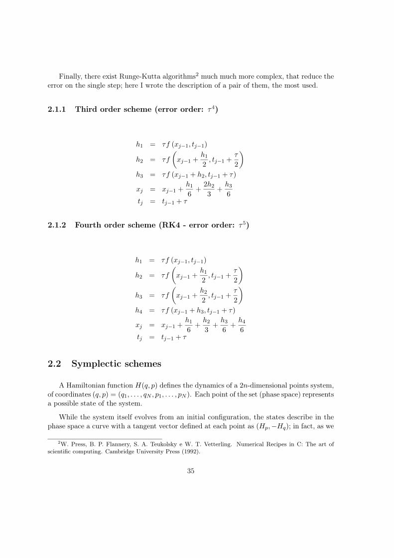
Finally, there exist Runge-Kutta algorithms2 much much more complex, that reduce theerror on the single step; here I wrote the description of a pair of them, the most used.

2.1.1 Third order scheme (error order: τ 4)

h1 = τf (xj−1, tj−1)

h2 = τf

(xj−1 +

h1

2, tj−1 +

τ

2

)h3 = τf (xj−1 + h2, tj−1 + τ)

xj = xj−1 +h1

6+

2h2

3+h3

6tj = tj−1 + τ

2.1.2 Fourth order scheme (RK4 - error order: τ 5)

h1 = τf (xj−1, tj−1)

h2 = τf

(xj−1 +

h1

2, tj−1 +

τ

2

)h3 = τf

(xj−1 +

h2

2, tj−1 +

τ

2

)h4 = τf (xj−1 + h3, tj−1 + τ)

xj = xj−1 +h1

6+h2

3+h3

6+h4

6tj = tj−1 + τ

2.2 Symplectic schemes

A Hamiltonian function H(q, p) defines the dynamics of a 2n-dimensional points system,of coordinates (q, p) = (q1, . . . , qN , p1, . . . , pN ). Each point of the set (phase space) representsa possible state of the system.

While the system itself evolves from an initial configuration, the states describe in thephase space a curve with a tangent vector defined at each point as (Hp,−Hq); in fact, as we

2W. Press, B. P. Flannery, S. A. Teukolsky e W. T. Vetterling. Numerical Recipes in C: The art ofscientific computing. Cambridge University Press (1992).

35

know, the Hamilton’s equations

p = −∂H∂q

q =∂H

∂p(2.2)

can be interpreted geometrically as the tangent vector of the evolution curve in the phasespace (as always, q is the position coordinate and p denotes the momentum).

The time evolution of Hamilton’s equations is a symplectomorphism, which means thatit preserves the symplectic two-form dp×dq. Simply said, a numerical scheme is a symplecticintegrator if it preserves this two-form.

In general, a function f in the phase space is symplectic if and only if

f ′(z)TJf ′(z) = J

in which J is defined as follows:

J =

(0 In

−In 0

)Most of the usual numerical methods, like the primitive Euler scheme and the Runge-

Kutta scheme, are not symplectic integrators.

How it works: a simple case

Let’s assume that the Hamiltonian is separable, so that

H(p, q) = T (p) + V (q) (2.3)

It’s not so rare that a Hamiltonian system can be expressed in this way, fortunately.Let’s define z = (q, p) so that

z = (q, p)

Using the formalism DH = , H eq. 2.2 can be expressed as

z = J∇H(z) = DHz = z,H(z) =∂(q, p)

∂q

∂H(q, p)

∂p− ∂(q, p)

∂p

∂H(q, p)

∂q=

= (1, 0)∂H(q, p)

∂p− (0, 1)

∂H(q, p)

∂q=

(∂H(q, p)

∂p, 0

)−(

0,∂H(q, p)

∂q

)=

=

(∂H

∂p,−∂H

∂q

)=

(∂T

∂p,−∂V

∂q

)(2.4)

The formal solution of this set of equations is

z(τ) = exp(τDH)z(0) (2.5)

36

When the Hamiltonian is in the form like 2.3, 2.5 is equivalent to

z(τ) = exp[τ(DT +DV )]z(0) (2.6)

The symplectic integrator scheme approximates this result 2.6 with the product

exp[τ(DT +DV )] =k∏i=1

exp(ciτDT ) exp(diτDV ) +O(τk+1

)(2.7)

in which ci and di are real numbers and k represents the order of the integrator.

Each of the operators exp(ciτDT ) and exp(diτDV ) is symplectic, so their product ap-pearing in the rhs of the 2.7 is a symplectic map too. From the previous descriptions we canextract many different integrators at different orders, each with its precise set of coefficientsci and di.

But let’s see what they give:

exp(ciτDT ) −→(qp

)7→

(q′

p′

)=

(q + τci

∂T∂p (p)

p

)and

exp(diτDV ) −→(qp

)7→

(q′

p′

)=

(q

p− τdi ∂V∂q (q)

)

An example

If T = p2/2m and V = kq2/2, we have:∂T

∂p=

p

m= p if we put m = 1

∂V

∂q= kq = F (this is an example of a spring)

So, knowing that at the first order ci = 1 and di = 1, we haveq + ∆t

∂T

∂p= q + ∆t · p

p−∆t∂V

∂q= p+ ∆t · F

For other informations, there exist a lot of articles3. But let’s see an example now.3For example, D. Donnelly, E. Rogers, Symplectic integrators: an introduction, Am. J. Phys. 73 (2005)

10.

37

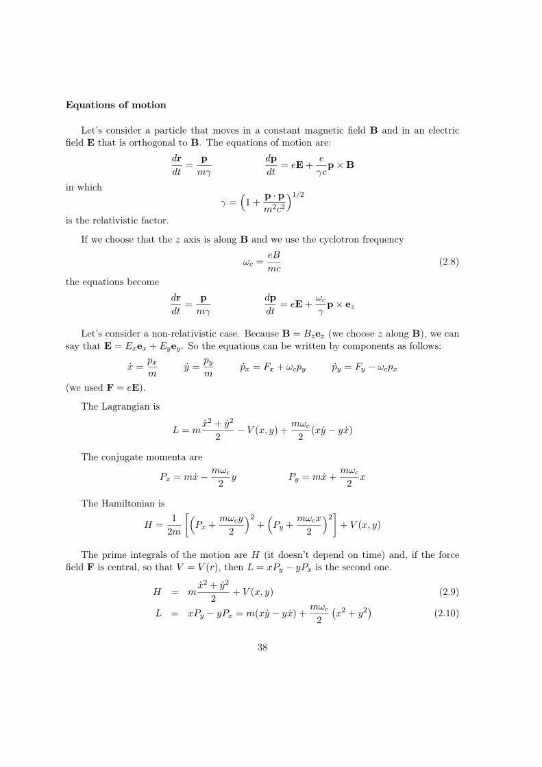
Equations of motion

Let’s consider a particle that moves in a constant magnetic field B and in an electricfield E that is orthogonal to B. The equations of motion are:

dr

dt=

p

mγ

dp

dt= eE +

e

γcp×B

in whichγ =

(1 +

p · pm2c2

)1/2

is the relativistic factor.

If we choose that the z axis is along B and we use the cyclotron frequency

ωc =eB

mc(2.8)

the equations becomedr

dt=

p

mγ

dp

dt= eE +

ωcγp× ez

Let’s consider a non-relativistic case. Because B = Bzez (we choose z along B), we cansay that E = Exex + Eyey. So the equations can be written by components as follows:

x =pxm

y =pym

px = Fx + ωcpy py = Fy − ωcpx

(we used F = eE).

The Lagrangian is

L = mx2 + y2

2− V (x, y) +

mωc2

(xy − yx)

The conjugate momenta are

Px = mx− mωc2y Py = mx+

mωc2x

The Hamiltonian is

H =1

2m

[(Px +

mωcy

2

)2+(Py +

mωcx

2

)2]

+ V (x, y)

The prime integrals of the motion are H (it doesn’t depend on time) and, if the forcefield F is central, so that V = V (r), then L = xPy − yPx is the second one.

H = mx2 + y2

2+ V (x, y) (2.9)

L = xPy − yPx = m(xy − yx) +mωc

2

(x2 + y2

)(2.10)

38

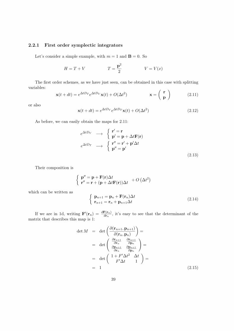
2.2.1 First order symplectic integrators

Let’s consider a simple example, with m = 1 and B = 0. So

H = T + V T =p2

2V = V (x)

The first order schemes, as we have just seen, can be obtained in this case with splittingvariables:

x(t+ dt) = e∆tDT e∆tDV x(t) +O(∆t2) x =

(rp

)(2.11)

or alsox(t+ dt) = e∆tDV e∆tDTx(t) +O(∆t2) (2.12)

As before, we can easily obtain the maps for 2.11:

e∆tDV −→

r′ = rp′ = p + ∆tF(r)

e∆tDT −→

r′′ = r′ + p′∆tp′′ = p′

(2.13)

Their composition is p′′ = p + F(r)∆tr′′ = r + (p + ∆tF(r))∆t

+O(∆t2

)which can be written as

pn+1 = pn + F(rn)∆trn+1 = rn + pn+1∆t

(2.14)

If we are in 1d, writing F′(rn) = dF(rn)drn

, it’s easy to see that the determinant of thematrix that describes this map is 1:

detM = det

(∂(rn+1,pn+1)

∂(rn,pn)

)=

= det

( ∂rn+1

∂rn

∂rn+1

∂pn∂pn+1

∂rn

∂pn+1

∂pn

)=

= det

(1 + F ′∆t2 ∆tF ′∆t 1

)=

= 1 (2.15)

39

For 2.12 the map is rn+1 = rn + pn∆tpn+1 = pn + F(rn+1)∆t

(2.16)

and the whole treatment is the same.

Action as a generator

An equivalent method would have required discretizing the action:

A(qa, qb) =

∫ tb

ta

L(q, q, t)dt (2.17)

that is the generator that transforms the system from (qa, pa) to (qb, pb).

So, if we discretize the action and we integrate with a first order method we find thegenerator of a canonical transformation that defines a first order integrator. Let’s considerta = t, tb = t + ∆t, q(ta) = qn and q(tb) = qn+1. The first derivative of q, q = p, can beapproximated with (qn+1 − qn)/∆t.

In this way, to solve

A(qn, qn+1) =

∫ t+∆t

t(T (p)− V (q))dt =

∫ t+∆t

t

(q2

2− V (q)

)dt = An +O

(∆t2

)(2.18)

we can use a first order approximation (rectangular):

An =(qn+1 − qn)2

2∆t− V (qn)∆t (2.19)

or

An =(qn+1 − qn)2

2∆t− V (qn+1)∆t (2.20)

It’s easy to verify from 2.18 that

pn = − ∂A∂qn

and pn+1 =∂A

∂qn+1

and so we find this relations for 2.19:

pn+1 =∂A

∂qn+1=qn+1 − qn

∆tand pn = − ∂A

∂qn=qn+1 − qn

∆t+dV (qn)

dqn∆t (2.21)

pn+1 = pn − V ′(qn)∆tqn+1 = qn + pn+1∆t

(2.22)

while for 2.20 those are:

pn+1 =∂A

∂qn+1=qn+1 − qn

∆t− dV (qn+1)

dqn+1∆t and pn =

∂A

∂qn=qn+1 − qn

∆t(2.23)

qn+1 = qn + pn∆tpn+1 = pn − V ′(qn+1)∆t

(2.24)

40

Extension to B fields

When there’s a B field the generalization of the previous algorithm is pretty neat at thefirst order. The two symplectic integrators 2.14 and 2.16 become

pn+1 = pn + E(rn)∆t+ ωcpn × ez∆trn+1 = rn + pn+1∆t

(2.25)

and rn+1 = rn + pn∆tpn+1 = pn + E(rn+1)∆t+ ωcpn+1 × ez∆t

(2.26)

in which E = E(r) is a central external force.

This second 2.26 integrator, as we can see, is not explicit but it can become so thanksto the fact that it’s linear in the momentum. They’re not symplectic: to get a symplecticversion we have to start from the action, which now is:

An =(rn+1 − rn)2

2∆t− V (rn)∆t+

ωc2rn × (rn+1 − rn) · ez (2.27)

or

An =(rn+1 − rn)2

2∆t− V (rn+1)∆t+

ωc2rn+1 × (rn+1 − rn) · ez (2.28)

The equations that we get from these actions are

Pn+1 =∂A

∂rn+1and Pn = − ∂A

∂rn+1(2.29)

in which P is not the momentum but

P = p +ωc2ez × r (2.30)

2.2.2 Second order symplectic integrators

x(t+ dt) = e∆t2DV︸ ︷︷ ︸C

e∆tDT︸ ︷︷ ︸B

e∆t2DV︸ ︷︷ ︸A

x(t) +O(∆t3) x =

(rp

)(2.31)

A :

r′ = r

p′ = p + ∆t2 F(r)

A+B :

r′′ = r′ + p′∆t = r + ∆t

(p + ∆t

2 F(r))

p′′ = p′ = p + ∆t2 F(r)

A+B + C :

r′′′ = r′′ = r + ∆t

(p + ∆t

2 F(r))

p′′′ = p′′ + ∆t2 F(r′′) = p + ∆t

2 F(r) + ∆t2 F

(r + ∆t

(p + ∆t

2 F(r)))(2.32)

41

This can be better written asrn+1 = rn + pn+1∆t+ F(rn)∆t

2

pn+1 = pn + ∆t2 F(rn) + ∆t

2 F(rn+1)(2.33)

Let’s calculate the determinant of the matrix that describes this map:

detM = det

(∂(rn+1,pn+1)

∂(rn,pn)

)=

= det

( ∂rn+1

∂rn

∂rn+1

∂pn∂pn+1

∂rn

∂pn+1

∂pn

)=

= det

(1 + F′(rn)∆t2

2 ∆t

F′(rn)∆t2 + ∆t

2 F′(rn+1)∂rn+1

∂rn1 + ∆t

2 F′(rn+1)∂rn+1

∂pn

)=

= det

(1 + F′(rn)∆t2

2 ∆t∆t2

[F′(rn) + F′(rn+1)∂rn+1

∂rn

]1 + ∆t

2 F′(rn+1)∂rn+1

∂pn

)=

= det

(1 + F′(rn)∆t2

2 ∆t∆t2

[F′(rn) + F′(rn+1)

(1 + F′(rn)∆t2

2

)]1 + ∆t2

2 F′(rn+1)

)=

= 1 + F′(rn)∆t2

2+

∆t2

2F′(rn+1) +

∆t4

4F′(rn)F′(rn+1) +

− ∆t2

2

[F′(rn) + F′(rn+1) +

∆t2

2F′(rn)F′(rn+1)

]=

= 1 (2.34)

2.3 Leapfrog integrators

Leapfrog integration is another way to solve ODEs. It is based on calculating positionsand velocities at interleaved time points, in such a way that they leapfrog over each other.

There exist schemes that are accurate at the second order both in space and time andare computationally light. They are often called staggered leapfrog algorithms.

Using values of un at time tn we can calculate currents (fluxes) Fj,n. Then, we calculatethe new values using the flux at the middle point, using the following algorithm:

uj,n+1 − uj,n−1 = −∆t

∆x(Fj+1,n − Fj−1,n)

This algorithm requires double the storage: we need to save both un−1 and un to calculateun+1

42

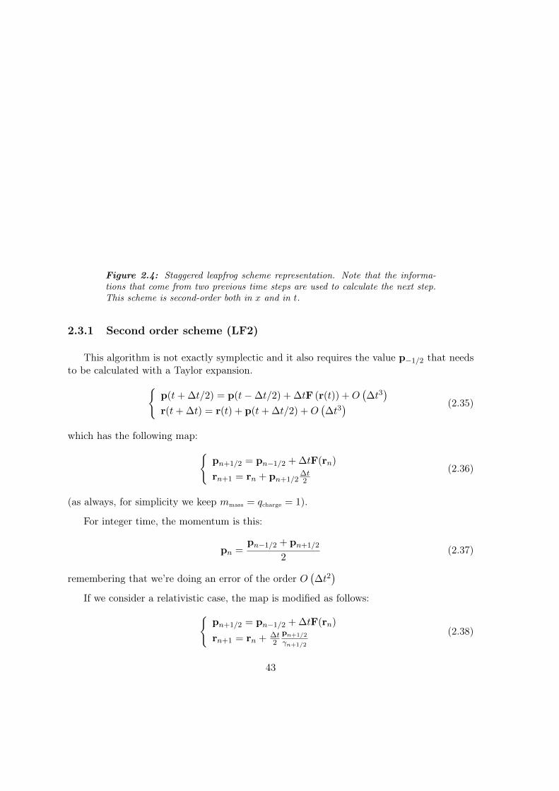
Figure 2.4: Staggered leapfrog scheme representation. Note that the informa-tions that come from two previous time steps are used to calculate the next step.This scheme is second-order both in x and in t.

2.3.1 Second order scheme (LF2)

This algorithm is not exactly symplectic and it also requires the value p−1/2 that needsto be calculated with a Taylor expansion.

p(t+ ∆t/2) = p(t−∆t/2) + ∆tF (r(t)) +O(∆t3

)r(t+ ∆t) = r(t) + p(t+ ∆t/2) +O

(∆t3

) (2.35)

which has the following map:pn+1/2 = pn−1/2 + ∆tF(rn)

rn+1 = rn + pn+1/2∆t2

(2.36)

(as always, for simplicity we keep mmass = qcharge = 1).

For integer time, the momentum is this:

pn =pn−1/2 + pn+1/2

2(2.37)

remembering that we’re doing an error of the order O(∆t2

)If we consider a relativistic case, the map is modified as follows:

pn+1/2 = pn−1/2 + ∆tF(rn)

rn+1 = rn + ∆t2

pn+1/2

γn+1/2

(2.38)

43

in which Fn = En + pnγn×Bn so that pn+1/2 = pn−1/2 + ∆t

(En +

pn−1/2+pn+1/2

2γn×Bn

)rn+1 = rn + ∆t

2

pn+1/2

γn+1/2

(2.39)

To solve the implicit equation for pn±1/2, instead of using 2.37, we can write pn as ahalf-step advancement over pn−1/2, obtaining a new but simpler implicit equation:

pn = pn−1/2 +∆t

2

(En +

pnγn×Bn

)(2.40)

Setting:

β = ∆t/2

p∗ = pn−1/2 + βEn (2.41)b = βBn/γn

equation 2.40 can be rewritten in this way:

pn = p∗ + pn × b (2.42)

or also:

p∗ = pn − pn × b (2.43)pn × b = pn − p∗ (2.44)

Multiplying on the right ×b the 2.43

p∗ × b = pn × b− (pn × b)× b (2.45)

Using the vector identity

C× (B×A) = A× (B×C) = B(A ·C)−C(A ·B)

we can rewrite the (pn × b)× b term as

(pn × b)× b = b× (pn × b) = pn(b · b)− b(b · pn) =

= pnb2 − b(b · pn) (2.46)

If we multiply the 2.43 by ·b on the right we get

p∗ · b = pn · b− (pn × b) · b︸ ︷︷ ︸it’s 0 by definition

(2.47)

44

so thatp∗ · b = pn · b (2.48)

Combining 2.46 with 2.48 we get

b× (pn × b) = pnb2 − b(b · p∗)

pnb2 = b× (pn × b) + b(b · p∗)

Using 2.44 we get

b2pn = b× (pn − p∗) + b(b · p∗)b2pn − b× pn = −b× p∗ + b(b · p∗)b2pn + pn × b = p∗ × b + b(b · p∗)

Applying 2.44 again it becomes

b2pn + pn − p∗ = p∗ × b + b(b · p∗)pn(b2 + 1) = p∗ + p∗ × b + b(b · p∗)

and finally

pn =1

b2 + 1[p∗ + p∗ × b + b(b · p∗)] (2.49)

To solve 2.40 we are more interested in pn × b. So let’s multiply 2.49 ×b:

pn × b =1

b2 + 1[p∗ + p∗ × b]× b (2.50)

Inserting 2.50 in 2.39 gives the final expression for the second order leapfrog algorithm:

pn+1/2 = pn−1/2 + ∆tEn +1

b2 + 1(p∗ + p∗ × b)× b (2.51)

Thanks to 2.41,

2p∗ = 2pn−1/2 + ∆tEn −→ pn−1/2 + ∆tEn = 2p∗ − pn−1/2

so that we can write the whole solution in terms of pn−1/2 and p∗, which are known:

pn+1/2 = 2p∗ − pn−1/2 +1

b2 + 1(p∗ + p∗ × b)× b (2.52)

Of course, we could have done similar calculations with an inverse leapfrog:rn+1/2 = rn−1/2 + ∆tpnγnpn+1 = pn + ∆tF(rn+1/2)

(2.53)

45

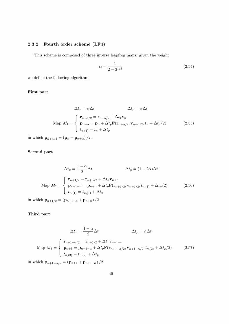
2.3.2 Fourth order scheme (LF4)

This scheme is composed of three inverse leapfrog maps: given the weight

α =1

2− 21/3(2.54)

we define the following algorithm.

First part

∆tx = α∆t ∆tp = α∆t

Map M1 =

rn+α/2 = rn−α/2 + ∆txvn

pn+α = pn + ∆tpF(rn+α/2,vn+α/2, tn + ∆tp/2)

tn,(1) = tn + ∆tp

(2.55)

in which pn+α/2 = (pn + pn+α) /2.

Second part

∆tx =1− α

2∆t ∆tp = (1− 2α)∆t

Map M2 =

rn+1/2 = rn+α/2 + ∆txvn+α

pn+1−α = pn+α + ∆tpF(rn+1/2,vn+1/2, tn,(1) + ∆tp/2)

tn,(1) = tn,(1) + ∆tp

(2.56)

in which pn+1/2 = (pn+1−α + pn+α) /2

Third part

∆tx =1− α

2∆t ∆tp = α∆t

Map M3 =

rn+1−α/2 = rn+1/2 + ∆txvn+1−α

pn+1 = pn+1−α + ∆tpF(rn+1−α/2,vn+1−α/2, tn,(2) + ∆tp/2)

tn,(3) = tn,(2) + ∆tp

(2.57)

in which pn+1−α/2 = (pn+1 + pn+1−α) /2

46

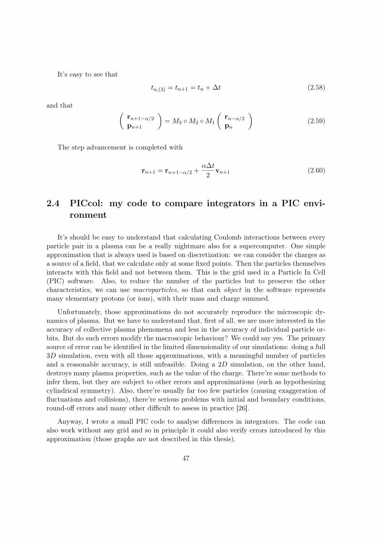
It’s easy to see that

tn,(3) = tn+1 = tn + ∆t (2.58)

and that (rn+1−α/2pn+1

)= M3 M2 M1

(rn−α/2pn

)(2.59)

The step advancement is completed with

rn+1 = rn+1−α/2 +α∆t

2vn+1 (2.60)

2.4 PICcol: my code to compare integrators in a PIC envi-ronment

It’s should be easy to understand that calculating Coulomb interactions between everyparticle pair in a plasma can be a really nightmare also for a supercomputer. One simpleapproximation that is always used is based on discretization: we can consider the charges asa source of a field, that we calculate only at some fixed points. Then the particles themselvesinteracts with this field and not between them. This is the grid used in a Particle In Cell(PIC) software. Also, to reduce the number of the particles but to preserve the othercharacteristics, we can use macroparticles, so that each object in the software representsmany elementary protons (or ions), with their mass and charge summed.

Unfortunately, those approximations do not accurately reproduce the microscopic dy-namics of plasma. But we have to understand that, first of all, we are more interested in theaccuracy of collective plasma phenomena and less in the accuracy of individual particle or-bits. But do such errors modify the macroscopic behaviour? We could say yes. The primarysource of error can be identified in the limited dimensionality of our simulations: doing a full3D simulation, even with all those approximations, with a meaningful number of particlesand a reasonable accuracy, is still unfeasible. Doing a 2D simulation, on the other hand,destroys many plasma properties, such as the value of the charge. There’re some methods toinfer them, but they are subject to other errors and approximations (such as hypothesizingcylindrical symmetry). Also, there’re usually far too few particles (causing exaggeration offluctuations and collisions), there’re serious problems with initial and boundary conditions,round-off errors and many other difficult to assess in practice [26].

Anyway, I wrote a small PIC code to analyse differences in integrators. The code canalso work without any grid and so in principle it could also verify errors introduced by thisapproximation (those graphs are not described in this thesis).

47

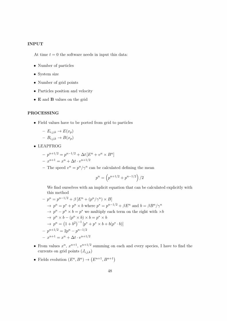
INPUT

At time t = 0 the software needs in input this data:

• Number of particles

• System size

• Number of grid points

• Particles position and velocity

• E and B values on the grid

PROCESSING

• Field values have to be ported from grid to particles

– Ei,j,k → E(xp)

– Bi,j,k → B(xp)

• LEAPFROG

– pn+1/2 = pn−1/2 + ∆t [En + vn ×Bn]

– xn+1 = xn + ∆t · vn+1/2

– The speed vn = pn/γn can be calculated defining the mean

pn =(pn+1/2 + pn−1/2

)/2

We find ourselves with an implicit equation that can be calculated explicitly withthis method

– pn = pn−1/2 + β [En + (pn/γn)×B]

→ pn = p∗ + pn × b where p∗ = pn−1/2 + βEn and b = βBn/γn

→ pn − pn × b = p∗ we multiply each term on the right with ×b→ pn × b− (pn × b)× b = p∗ × b→ pn =

(1 + b2

)−1[p∗ + p∗ × b+ b(p∗ · b)]

– pn+1/2 = 2pn − pn−1/2

– xn+1 = xn + ∆t · vn+1/2

• From values xn, xn+1, vn+1/2 summing on each and every species, I have to find thecurrents on grid points (Ji,j,k)

• Fields evolution (En, Bn)→(En+1, Bn+1

)48

– Bn = Bn−1/2 − 12∆t∇× En

– Bn+1/2 = Bn − 12∆t∇× En

– En+1 = En + ∆t[∇×Bn+1/2 − Jn+1/2

]– Bn+1 = Bn+1/2 −∆t∇× En+1

OUTPUT

As we can see from figures 2.5, 2.6 and 2.7, we can say that a 2nd order leapfrog algorithmis substantially similar to a symplectic integrator.

Figure 2.5: Leapfrog 2nd order (red) vs Runge-Kutta 4th order (blue) for primeintegrals, px, py, Py and H − Px.

49

Figure 2.6: Leapfrog 4th order (red) vs Runge-Kutta 4th order (blue) for primeintegrals, px, py, Py and H − Px.

Figure 2.7: Leapfrog 2nd order (red) vs symplectic 2nd order (blue) for primeintegrals, px, py, Py and H − Px.

50

CHAPTER 3

Protons transport

The main problem studied within this thesis is the transport of the protons obtainedfrom laser-plasma interactions.

This kind of problem is still an open question within the physics community: it’s reallycomplex and we’re still trying to understand which devices should be the best for this task.To make accelerated protons useful, in fact, we need to carry them away from the targetzone: we cannot install a post-acceleration device so close to the interaction point (and alsothe bunch would not be good enough at this point) and, for example, we couldn’t even askfor a patient that requires a proton-therapy to stay within this region with gas jets andpowerful electromagnetic devices.

So, we must be able to transport these bunches for at least a few dozens of centimeters.What could we use? In this chapter I will describe how we started looking at classical FODObeamlines (focusing-defocusing quadrupoles) and how we then arrived to the solenoid, basedon the experience that other groups made on this topic.

This study has been done using a code developed and extended by me during the periodof my thesis. It’s able to track particles independently when propagating along a beamlinecomposed of different magnetic elements. The newest version, written in C++, is parallelizedand uses some strictly defined interfaces to read input and write the simulations to disk, sothat it can work in the environment built with all the other codes of the group.

51

3.1 Transport of protons coming from TNSA regime

The main characteristic of an optically accelerated beam, in TNSA regime, is its expo-nential spectrum of energy, with a cutoff Emax(∞) [27]. What it’s really interesting is notthe upper cutoff Emax(∞), but the mean energy. For the injection it’s important that thebeam is almost monochromatic, but at the highest energies the intensities are really low. Infact

ρ(E) =dN

dE=E0

N0e−E/E0ϑ (Emax(∞)− E) (3.1)

If we suppose that Emax(∞) 〈E〉, the upper cut can be ignored and we immediately verifythat the total number of particles is given by

Ntot =

∫ ∞0

dN

dEdE = N0

∫ ∞0

e−udu = N0 (3.2)

Analogously, the total energy is:

Etot =

∫ ∞0

EdN

dEdE = N0 E0

∫ ∞0

u e−udu = N0 E0 (3.3)

The mean energy can be expressed as:

〈E〉 =Etot

Ntot= E0 (3.4)

The number of particles in a small interval [E,E + ∆E] is

N ([E,E + ∆E]) =

∫ E+∆E

EEdN

dEdE = N0

∫ (E+∆E)/E0

E/E0

e−udu ' N0∆E

E0e−E/E0 (3.5)

Let’s suppose that we want to select protons with an energy of E = 10 MeV and a spreadof 0.1 MeV, or 1%. Under these conditions the fraction n(E0) = N(E0)/N0 of protons atdifferent E0 mean energies is

n(2) = 6.7 10−5 n(2.5) = 1.8 10−4 n(3) = 3.6 10−4

n(4) = 8.2 10−4 n(5) = 1.3 10−3

We clearly see that if we start from N0 = 1011 protons we need to have a mean energythat is between 2.5 and 5 MeV, to have a minimum of 107 injectable protons, keeping underconsideration also the transport beamline and its losses.

There are two main types of target: solid targets and liquid hydrogen. From simulations[28] it’s clear that the mean energy is greater for liquid hydrogen: the percentage of the laserenergy converted into kinetic energy of protons reaches 10%.

52

We can estimate the number of protons that are accelerated knowing their mean energyand the energy in a laser pulse. For example, at the Dresden-Rossendorf (ZFD) researchcentre [29], the laser DRACO has an energy of 3 J and the mean energy of the protonsejected is 2 MeV: considering previous results, the transferred energy so is approximately0.3 J and the number of protons that we get is

N0 =0.1 Elaser

E0=

0.3 J2 MeV

=0.3 J

2× 1.6 10−13 J∼ 1013

Their data give us this numbers for the accelerated protons distribution:

dN

dE dΩ= 3 1011 e−E/E0 MeV−1 E0 = 1.7 MeV (3.6)

Unfortunately, they do not describe the angular distribution. If we assume it as uniformin the forward direction (angle = 2π), we have

N0 = 1.7× 2π × 3 1011 = 3 1012 (3.7)

If we consider a cone obtained with a collimator (iris) with |φ| ≤ 0.1 rad, that correspondsto an aperture of 2 × 0.1 × 180/π = 0.2 rad ∼ 11, the number of protons that we getaccording to Eq. 3.7 is N = 1.7 × 0.2 × 3 1011 ∼ 1011. The number of protons with anenergy of 10.0± 0.1 MeV is 2.6 107. We are within the limits, but with a strict margin. Wehave to consider that a uniform angular distribution means that only the 3% of the laserenergy is converted, instead of the commonly accepted 10%. So it’s possible that the energytransfer is less efficient for DRACO, that the spectrum underestimates the real values orthat the energy distribution is not uniform in angle.

3.2 Lilia and Prometheus

Our group works within the Lilia collaboration, aimed to simulate and do feasibilitystudies for the Flame laser at LNF (Frascati) [30], studying new gaseous targets and trans-port lines. We are also doing some feasibility studies for a new facility, Prometheus, basedon a high power laser, aimed to have proton bunches for biomedical studies and applications[31, 32]. This project is done in collaboration with the ENEA division in Bologna and someother private funds.

Lilia experiment aims to obtain significant advances in the knowledge of physical phe-nomena regarding laser-accelerated proton bunches. The objective is to get a beam withprotons of at least 50 MeV of energy and intensity in the order of 1013. To reach this target,many activities will be done regarding theoretical studies of laser-plasma interactions andnew regimes of accelerations, experimental studies of target configurations, focusing devicesand new kinds of detectors to analyse the beam obtained.

53

3.3 My experience at the Goethe University in Frankfurt

To do part of the work I went to the Frankfurt Goethe University. I worked there forsix weeks and my tasks were supposed to be mainly focused on the code check: in BolognaI worked on developing a new code, Propaga, started by Prof. Servizi, that tracks particlespropagating along a beamline.

Just few days before my departure, with Prof. G. Servizi we developed a tool to animatesimulated particles, using the passe-par-tout library developed by himself [33]. It took acouple of days while I was in Frankfurt to make the program working in a portable way.Previously, films were not reproducible on a machine different from the original creator andso I was not able to play them remotely.

After having fixed those problems, I went on comparing our results with LORASR andTrace-3D ones [34, 35]. Those are trusted codes that are used to design cavities and so theyare a great opportunity to find and fix any problem that could arise in our simulations. Thefirst software, in particular, belongs to the University of Frankfurt.

One way to do these first checks is to compare beam envelopes. Immediately, I discoveredthat I couldn’t get those graphs from our simulations, so I wrote a small tool to gather thatdata from our output and while I was developing it I also added the possibility to track onesingle custom defined particle along the whole beamline.

Using

σx = 〈x2〉 − 〈x〉 〈x〉σy = 〈y2〉 − 〈y〉 〈y〉σz = 〈z2〉 − 〈z〉 〈z〉σpx = 〈p2

x〉 − 〈px〉 〈px〉σpy = 〈p2

y〉 − 〈py〉 〈py〉σpz = 〈p2

z〉 − 〈pz〉 〈pz〉mx = 〈xpx〉 − 〈x〉 〈px〉my = 〈ypy〉 − 〈y〉 〈py〉mz = 〈zpz〉 − 〈z〉 〈pz〉

we defined emittances in this way:

εx =√σx σpx −m2

x

εy =√σy σpy −m2

y (3.8)

εz =√σz σpz −m2

z

54

3.3.1 BuGe: my bunch generator

In the beginning, when we started the checking of the code, we decided to use a uniformdistribution for the input bunch and not one of the realistic bunches that I had, producedby ALaDyn. In this way, bunches are better defined and their properties are completelyunder our control. But this also means that a bunch generator is needed, and so I wroteone from scratch recycling some number generator routines from previous works.

This work required a lot of time, because I had to learn particle distributions [36], inparticular the Kapchinskij-Vladimirskij one.

Kapchinskij-Vladimirskij distribution

In a paper presented in the International Conference on High-Energy Accelerators andInstrumentation at CERN in 1959, I. M. Kapchinskij and V. V. Vladimirskij discussed thespace charge significance to the beam cross-section in the stationary conditions for a definitephase volume of injected particles [37, 38].

They made the following assumptions when deducing their phase-space distributions ofparticles:

• the beam cross-section is appreciably smaller than the variation period of the focusingfield;

• the particles move only in the linear region of the external field close to the accelerator’saxis;

• the influence of the space charge is essential only at relatively small velocities, so thatit is assumed that the particle velocity is much below the velocity of light;

• the energy increment in a gap is sufficiently small, so that the period of synchrotronoscillations is much greater than the acceleration period.

In these assumptions, the equations of transversal oscillations for a particle propagatinginto magnetic quadrupole lenses may be expressed in the following form

d2x

dτ2+Qx(τ) · x+

eλ2

mc2· ∂UK∂x

= 0 (3.9)

d2y

dτ2+Qy(τ) · y +

eλ2

mc2· ∂UK∂y

= 0 (3.10)

(3.11)

where z is directed along the axis of the accelerator. The independent variable τ is definedas

τ =ct

λ

55

and

• e, m are charge and mass of the particle;

• λ is the wavelength of the high frequency accelerating field in free space;

• UK(x, y, z) is the potential of the field of the beam space charge.

• Qx(τ) = Q1(τ) +Q2(τ);

• Qx(τ) = Q1(τ)−Q2(τ);

where the functions Q1(τ) is the defocusing action of the accelerating gaps and Q2(τ) isdetermined by the focusing field:

Q1(τ) =eλ2

2mc2· ∂Ez(r, z, τ)

∂z

Q2(τ) = λ2 eβ

mc2·G · g(τ)

g(τ) has the period of the focusing field and changes within the limits |g(τ)| ≤ 1, G is themagnetic field gradient on the axis in the middle portion of the lens.

The period of the beam cross-section change has the same value order as the period ofthe focusing field; since the beam cross-section is substantially smaller than the period ofcross-section changes, the field of the space charge Ek changes much slower along the axis zthan along the axes x and y: ∣∣∣∣∂Ekz∂z

∣∣∣∣ ∣∣∣∣∂Exk∂x

∣∣∣∣ , ∣∣∣∣∂Eyk∂y

∣∣∣∣Thus

divE ≈ ∂Exk∂x

+∂Eyk∂y

from which∂2UK∂x2

+∂2UK∂y2

= −4π · ρ(x, y, z) (3.12)

Let’s assume that n(x, y, z, x, y, z) is the density of particle distribution in the phasespace of coordinates and velocities. According to Liouville’s theorem, the function n remainsconstant along the trajectory of the particle motion in the phase space, so that n dependsonly on the integrals of motion.

The space charge density in the beam ρ(x, y, z) is determined by the integral

ρ(x, y, z) = e

∫∫∫n(x, y, z, x, y, z) dxdydz (3.13)

56

The equations 3.9 and 3.10 should be solved jointly with equations 3.12 and 3.13, whichdetermine the potential of the space charge field UK(x, y, z), provided the phase density ofparticles n is a function of the integrals of motion of equations 3.9 and 3.10.

The integration of equations 3.9 and 3.10 will be materially simplified if we introducea special assumption regarding the law of particle distribution in the phase space; namely,if we choose such a dependence of phase density upon the integrals of motion so that theybecome linear in the separated variables.

Let’s consider equation 3.9; if it’s linear regarding to the function x(τ), then it’s possibleto choose a pair of complex-conjugated fundamental solutions

χx(τ) = δx(τ) eiψx(τ)

χ∗x(τ) = δx(τ) e−iψx(τ)

which make it possible to express any real solution with arbitrary initial conditions as

x(τ) = Ax · δx(τ) cos [ψx(τ) + θx] (3.14)

The Wronskian of the functions χx and χ∗x, which is defined as

W (f1, f2)(x) = det

∣∣∣∣ f1(x) f2(x)f ′1(x) f ′2(x)

∣∣∣∣is a well known constant value. Let’s put

χxdχ∗xdτ− χ∗x

dχxdτ

= −2i (3.15)

It follows from 3.15 thatdψxdτ

=1

δ2x

The solution of the equation 3.10 has the analogous form

y(τ) = Ay · δy(τ) cos [ψy(τ) + θy]

dψydτ

=1

δ2y

(3.16)

The values Ax, Ay, θx, θy depend only upon the initial conditions and consequentlyare the integrals of motion. The phases of the transversal oscillations of particles θx, θyare cyclic functions of the initial coordinates and velocities. It’s natural to suppose thatthe function of density distribution n depends only upon the integrals of motion Ax, Aywhich are characteristic of the transversal oscillation intensity. The oscillation phases θx, θymay be of arbitrary value. We shall obtain the expressions for the integrals Ax and Ay byeliminating from the functions (x(τ), dx/dτ) and (y(τ), dy/dτ) the phases (θx, θy):

57

(δxx− δxx

)2+

(x

δx

)2

= A2x(

δyy − δyy)2

+

(y

δy

)2

= A2y

Let’s now assume that the particle distribution density in phase space depends upon theintegrals of motion in the following way:

n = n0 δ(F − F0)

where in a general caseF = A2

x + s A2y

and δ is the usual δ-function. We shall assume further on that s = 1, so we get

F = A2x +A2

y

Thus, due to the assumption, all the particles in a four-dimensional phase-space x, y, x,y are situated on the surface of the ellipsoid(

δxx− δxx)2

+

(x

δx

)2

+(δyy − δyy

)2+

(y

δy

)2

= F

The projections of the representing points on the plane x, x, y, y fill up the correspondingellipses (

δxx− δxx)2

+

(x

δx

)2

= A2x,max(

δyy − δyy)2

+

(y

δy

)2

= A2y,max

Code development

Using some defined conditions upon the KV ellipses (Twiss parameters), I built a re-ally simple bunch generator that is able to create uniformly distributed bunches in eachdimension (x, y, z, px, py, pz).

x2

R2+x′2

θ2+y2

R2+y′2

θ2= 1 (3.17)

where θ is the opening angle and R is the maximum beam radius (in x and y).

58

Of course, the code implementation differs a little from this equation, mainly becauseI accepted not only the real surface of the ellipsoid but a region that is between 0.95 and1.00. Imposing the equality to 1 would have meant to reject most of the particles generatedby our Monte-Carlo number generator, while accepting a skin larger than 0.05 could causebad effects because the projections would have not been uniform again.

With these conditions, the plots of the coordinates of the generated particles becameacceptable. In figures [3.1 and 3.2] there’s an example of a uniformly distributed bunch,made with these parameters:

• bunch radius: 60 nm

• bunch length: 22 nm

• average energy: ∼ 10.1 MeV

• energy spread: ∼ 6 %

-60

-40

-20

0

20

40

60

-60 -40 -20 0 20 40 60

y po

sitio

n (µ

m)

x position (µm)

x-y

0

5

10

15

20

25

-60 -40 -20 0 20 40 60

z po

sitio

n (µ

m)

x position (µm)

x-z

Figure 3.1: On the left, xy distribution of uniformly generated particles; on theright, the xz distribution.

3.4 Propaga

3.4.1 Introduction to our code

Our group in Bologna developed a code for particle tracking along a beamline. Its nameis Propaga. It was written quickly, but with the intention to create a good software and notto replace it very soon.

When I arrived in Frankfurt in June of this year, the status of the code development wasconsidered good: it was able to track particles along many types of magnetic element, like

59

0

200

400

600

800

1000

1200

1400

1600

1800

2000

0.14 0.142 0.144 0.146 0.148 0.15 0.152

Fre

quen

cy

βz (pz/mpc)

Energy distribution

-0.015

-0.01

-0.005

0

0.005

0.01

0.015

-0.015 -0.01 -0.005 0 0.005 0.01 0.015

β y(py/mpc)

βx (px/mpc)

px-py

Figure 3.2: On the left, energy distribution of uniformly generated particles; onthe right, transverse momentum (βx and βy)

quadrupoles (focusing and defocusing) and solenoids. It lacked, and still lacks, any kind ofspace-charge effects treatment and RF cavities.

To begin the checks of our code, I compared it with some simulations done with ASTRA,a tool from DESY that I started learning before leaving to Frankfurt [39, 40].

The first test was based on the PHELIX [41] configuration: a really simple beamline witha solenoid with a length of 72 mm placed 15 mm after the target. Because our solenoid usedan hard edge approximation, we chose a B-field of 17.8 T, a field that should be enough tofocus a bunch with a reference energy of 10.1 MeV ±6% and an opening angle of 90 mrad,which describes approximately the strength of the real solenoid.

As you can see from the picture 3.3, we were in good agreement when comparing withASTRA, used with an input file that asked for an hard edge approximation and that disabledthe space-charge effects: the problem is that none of the two software focused the bunch asrequired, even if our approximation were ignoring defocusing effects like space charges: ifwrong, we should have seen more focusing than real, not absence of focus!

So I started analysing deeply how our code works, hoping to find where the problemswere, while also studying the subject to understand why ASTRA is failing too.

3.4.2 Maps of the beamline elements

Our code uses a time integration, not a spatial one like most of other tools do. So itwas a bit difficult to compare nearly all of the literature with our calculations, because ofdifferent approximations and different treatments of the matrices that map each element ofa beamline [42, 43].

60

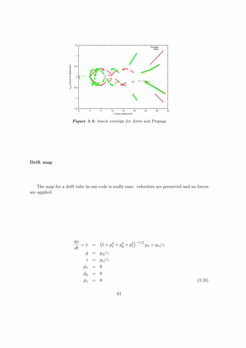
-1.5

-1

-0.5

0

0.5

1

1.5

-5 0 5 10 15 20 25 30 35

x max

(bun

ch e

nvel

ope)

[cm

]

z mean position [cm]

PropagaAstra

Figure 3.3: bunch envelope for Astra and Propaga

Drift map

The map for a drift tube in our code is really easy: velocities are preserved and no forcesare applied.

dx

dt= x =

(1 + p2

x + p2y + p2

z

)−1/2px = px/γ

y = py/γ

z = pz/γ

px = 0

py = 0

pz = 0 (3.18)

61

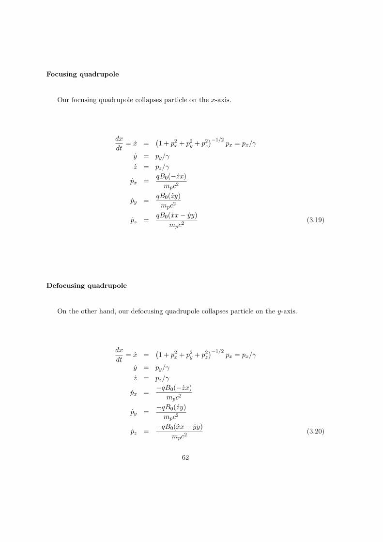
Focusing quadrupole

Our focusing quadrupole collapses particle on the x-axis.

dx

dt= x =

(1 + p2

x + p2y + p2

z

)−1/2px = px/γ

y = py/γ

z = pz/γ

px =qB0(−zx)

mpc2

py =qB0(zy)

mpc2

pz =qB0(xx− yy)

mpc2(3.19)

Defocusing quadrupole

On the other hand, our defocusing quadrupole collapses particle on the y-axis.

dx

dt= x =

(1 + p2

x + p2y + p2

z

)−1/2px = px/γ

y = py/γ

z = pz/γ

px =−qB0(−zx)

mpc2

py =−qB0(zy)

mpc2

pz =−qB0(xx− yy)

mpc2(3.20)

62

Solenoid map

The solenoid was the only device really tested in Frankfurt. At the beginning, the mapwas only the following:

dx

dt= x =

(1 + p2

x + p2y + p2

z

)−1/2px = px/γ

y = py/γ

z = pz/γ

px =qB0

mpc2· pyγ

py = − qB0

mpc2· pxγ

pz = 0 (3.21)

But, as we said, with such a map we were not able to describe a focusing effect that weshould get with those parameters. After many talks within the group, we found that wewere not considering the fringe fields, that describe the curvature of the field lines at thebeginning and at the end of the solenoid [44] (Figure 3.4).

Figure 3.4: Schematic representation of the focusing effect of a solenoid

As noted during our discussions, not considering them is not a valid approximation, itmeans not considering real important physical effects, without them we do not even haveany focusing from the solenoid.

Adding them to our software required that I learned it deeply, because it needed somecorrections and extensions. In literature, fringe fields matrices are always described as aninstant transformation on a space plane and so they do not require any time integration.

But let’s look at a more detailed treatment of the fringing fields.

63

Fringe fields of the solenoid

Defining the potential vector B = ∇×A, owing to the fact that B is defined as constantin the solenoid, we have: ∮

A · dl =

∫B0 · dΣ

A 2πr = B0 πr2

A =B0 · r

2(3.22)

Starting from the relativistic Lagrangian

L = −m0c2√

1− β2 − eA · v

the canonical momenta in the transverse plane are defined by

px =∂L∂x

= γm0vx + eAx

py =∂L∂y

= γm0vy + eAy (3.23)

As we know, any magnetic field will not give energy to our particles. So we have toconsider angular momentum and energy conservation; owing to the cylindrical symmetry wecan write

1

2mv2

φ +1

2mv2

r +1

2mv2

z = const.

for the energy andr× p = r · pφ = const.

for the angular momentum. This because

dL

dt= Mtot

where L is the angular momentum and Mtot the momentum of the external forces:

Mtot = r× Ftot

Because of the fact that the magnetic force is a centripetal force, we have r//F and soMtot = 0, that means

dL

dt= 0

64

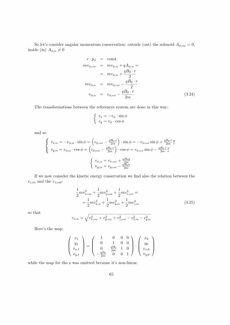
So let’s consider angular momentum conservation: outside (out) the solenoid Aφ,out = 0,inside (in) Aφ,in 6= 0

r · pφ = const.mvφ,out = mvφ,in + qAφ,in =

= mvφ,in +qB0 · r

2

mvφ,in = mvφ,out −qB0 · r

2

vφ,in = vφ,out −qB0 · r

2m(3.24)

The transformations between the references system are done in this way:vx = −vφ · sinφvy = vφ · cosφ

and so vx,in = −vφ,in · sinφ =(vφ,out − qB0·r

2m

)· sinφ = −vφ,out sinφ+ qB0·r

2myr

vy,in = vφ,in · cosφ =(vφ,out − qB0·r

2m

)· cosφ = vφ,out sinφ− qB0·r

2mxr

vx,in = vx,out + qB0y2m

vy,in = vy,out − qB0x2m

If we now consider the kinetic energy conservation we find also the relation between thevz,in and the vz,out:

1

2mv2

x,out +1

2mv2

y,out +1

2mv2

z,out =

=1

2mv2

x,in +1

2mv2

y,in +1

2mv2

z,in (3.25)

so thatvz,in =

√v2x,out + v2

y,out + v2z,out − v2

x,in − v2y,in

Here’s the map: x1

y1

vx,1vy,1

=

1 0 0 00 1 0 0

0 qB0

2m 1 0

− qB0

2m 0 0 1

·

x0

y0

vx,0vy,0

while the map for the z was omitted because it’s non-linear.

65

When the particle is coming out from the solenoid this is the map for the fringing field:x2

y2

vx,2vy,2

=

1 0 0 00 1 0 0

0 − qB0

2m 1 0qB0

2m 0 0 1

·

x1

y1

vx,1vy,1

3.5 Our simulations

In this paragraph I’ll recap all the simulations that we have done for this transportproblem.

3.5.1 Bunches from PIC simulations

First of all, we started using bunches obtained by Carlo Benedetti using ALaDyn code[45]. Those are realistic bunches, and because of this fact they were really hard to use whencross-checking results with other software (there’s no way to understand at first sight someeffects).

bunch3D v1

This is the original bunch. In fig. 3.5 there’re the position distribution in x and yand in x and z, while in fig. 3.6 there’re the energy distribution, obtained via βz (in ourcode, the momenta are pure numbers, because they are divided by mpc), and the transversemomentum distribution, βx vs βy.

-25

-20

-15

-10

-5

0

5

10

15

20

25

-25 -20 -15 -10 -5 0 5 10 15 20 25

y po

sitio

n (µ

m)

x position (µm)

x-y

2

4

6

8

10

12

14

16

18

20

22

-25 -20 -15 -10 -5 0 5 10 15 20 25

z po

sitio

n (µ

m)

x position (µm)

x-z

Figure 3.5: bunch #1 particle distribution in xy (left) and xz (right)

66

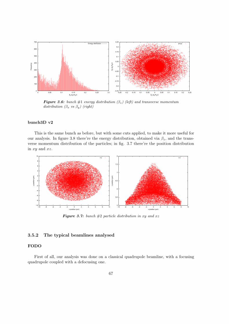
0

100

200

300

400

500

600

700

0 0.05 0.1 0.15 0.2 0.25 0.3

Fre

quen

cy

βz (pz/mpc)

Energy distribution

-0.25

-0.2

-0.15

-0.1

-0.05

0

0.05

0.1

0.15

0.2

0.25

-0.25 -0.2 -0.15 -0.1 -0.05 0 0.05 0.1 0.15 0.2 0.25

β y(py/mpc)

βx (px/mpc)

px-py

Figure 3.6: bunch #1 energy distribution (βz) (left) and transverse momentumdistribution (βx vs βy) (right)

bunch3D v2

This is the same bunch as before, but with some cuts applied, to make it more useful forour analysis. In figure 3.8 there’re the energy distribution, obtained via βz, and the trans-verse momentum distribution of the particles; in fig. 3.7 there’re the position distributionin xy and xz.

-10

-8

-6

-4

-2

0

2

4

6

8

10

-10 -8 -6 -4 -2 0 2 4 6 8 10

y po

sitio

n (µ

m)

x position (µm)

x-y

5

5.5

6

6.5

7

7.5

8

-10 -8 -6 -4 -2 0 2 4 6 8 10

z po

sitio

n (µ

m)

x position (µm)

x-z

Figure 3.7: bunch #2 particle distribution in xy and xz

3.5.2 The typical beamlines analysed

FODO

First of all, our analysis was done on a classical quadrupole beamline, with a focusingquadrupole coupled with a defocusing one.

67

Characteristics of the beamline:

• focusing quadrupole length: 10 cm

• focusing quadrupole field gradient: 30 T/m

• defocusing quadrupole length: 10 cm

• defocusing quadrupole field gradient: 30 T/m

Results were not really very promising, because this beamline required very high gradi-ents to keep emittance under control. As we can see from literature, in fact, quadrupoleswith a so high gradient are still under investigations [46].

I+FODO+I

The analysis proceeded inserting two irises, at the beginning and at the end of thebeamline, to further reduce the emittance. Unfortunately, with this choice, really very fewprotons survived!

Characteristics of the beamline:

• first iris radius: 0.5 mm

• second iris radius: 0.5 mm

Solenoid

Starting from my experience in Frankfurt, we began considering solenoids as effectivefocusing elements. We started with a really simple hard edge model of the solenoid, likethose used for quadrupoles.

First of all we started with a configuration like Fig. 3.9. We immediately dropped bothirises, because the losses were exaggerate.

After these simulations, we changed our transport beamline, simplifying with only aniris at the beginning and implementing more realistic models for the solenoid.

Characteristics of the beamline:

• initial drift of 1 cm

• solenoid length: 20 cm

• solenoid B-field: 30 T

68

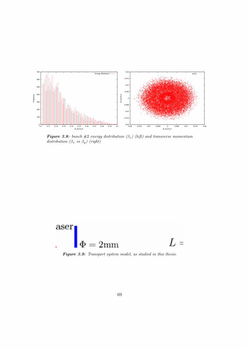
0

100

200

300

400

500

600

700

0.1 0.11 0.12 0.13 0.14 0.15 0.16 0.17 0.18 0.19 0.2

Fre

quen

cy

βz (pz/mpc)

Energy distribution

-0.02

-0.015

-0.01

-0.005

0

0.005

0.01

0.015

0.02

-0.02 -0.015 -0.01 -0.005 0 0.005 0.01 0.015 0.02

β y(py/mpc)

βx (px/mpc)

px-py

Figure 3.8: bunch #2 energy distribution (βz) (left) and transverse momentumdistribution (βx vs βy) (right)

Figure 3.9: Transport system model, as studied in this thesis.

69

I+Solenoid

As just said, we tried also to further reduce emittances with an iris at the beginning ofthe solenoid.

Characteristics of the beamline:

• iris radius: 0.5 mm

Solenoid with fringing fields - Phelix beamline configuration

Describing the solenoids in a more realistic way was a key to the latest simulations. InFrankfurt I cross-checked our code with the kick-model at the beginning and at the end ofthe solenoid, using the parameters of the Phelix beamline from GSI.

• initial drift of 15 mm

• solenoid length: 72 mm

• solenoid B-field: 17.8 T (hard edge with kick model for fringing fields)

3.5.3 Status of the code at the end of the Frankfurt period

At the end of my period spent in Frankfurt dealing with those problem, our code dealtbetter with solenoids and passed checks against LORASR and Trace-3D codes. In the figure[3.10] I made a comparison between LORASR and PROPAGA and everything was reallybetter. Also, we did some benchmarks with a custom-made bunch, with a 5 mm radiusmade of particles without transversal momentum, to see the differences between an hardedge model with and without the fringing fields treatment. As we can see from figure[3.11], the solenoid model without fringe fields is unable to focus this kind of bunches, whileexperimentally they’re focused. It’s a clear demonstration about the importance of thesecorrections in the simulations.

3.5.4 Simulations with K-V bunches

To better compare our code with ASTRA, LORASR and Trace 3-D, I also analysed manytimes my transport code with many different K-V distributed bunch and different beamlines.We can see some graphs in fig. 3.12, in which we can see how the bunch envelope is differentfor the same bunch when it’s propagating into a beamline composed of only a solenoid atdifferent B-field configurations.

70

-0.25

-0.2

-0.15

-0.1

-0.05

0

0.05

0.1

0.15

0.2

0.25

0 5 10 15 20

bunc

h en

velo

pe (

cm)

z position (cm)

Propaga xmaxLorasr xmax(+)Lorasr xmax(-)

Figure 3.10: bunch envelope (x along z) for a bunch with an energy of 10 MeV,a spread of 2% propagating in the Phelix beamline.

-1

-0.8

-0.6

-0.4

-0.2

0

0.2

0.4

0.6

0.8

1

0 5 10 15 20 25

bunc

h en

velo

pe (

cm)

z position (cm)

bunch envelope Propaga, HardEdgebunch envelope Astra, HardEdge

bunch envelope Propaga, Smooth

Figure 3.11: bunch envelope (x along z) for a bunch without transversal mo-mentum and an initial radius of 5 mm, in the Phelix beamline configuration.

71

-0.6

-0.4

-0.2

0

0.2

0.4

0.6

0 5 10 15 20 25

x max

(bun

ch e

nvel

ope)

[cm

]

z position [cm]

BE-uniform-oa45-de1-17.8TBE-uniform-oa45-de1-20TBE-uniform-oa45-de1-25TBE-uniform-oa45-de1-30T

Figure 3.12: bunch envelope for a uniform KV bunch with an energy spread of1% and an opening angle (x′/βzeta) of 45 mrad at different magnetic fields

72

3.5.5 The hard edge approximation removed

Back in Italy, I worked on a much more realistic description of the field, to remove thehard edge approximation. Using a function designed to make a smoother Heaviside theta,

f(z, z0, λ) =1(

1 + e−(z−z0)/λ) (3.26)

which then gives a smoother delta:

f ′(z, z0, λ) =1

λ

e−(z−z0)/λ(1 + e−(z−z0)/λ

)2 (3.27)

we can now design a curve for the B-field that does not have any discontinuity. We canwrite the B field in this way:

B =

BρBφBz

(3.28)

so that the smoothed Bz is:

Bz = B0 (f(z, 0, λ)− f(z, Ls, λ)) (3.29)

From the divergence operator rewritten in cylindrical coordinates we get that

∇ ·B =1

ρ∂ρ (ρBρ) +

1

ρ∂φ (Bφ) + ∂zBz = 0 (3.30)

so that we can write, after having imposed Bφ = 0, a Bρ like this:

Bρ = −1

2B0ρ

(f ′(z, 0, λ)− f ′(z, Ls, λ)

)(3.31)

so thatBx = −1

2B0x

(f ′(z, 0, λ)− f ′(z, Ls, λ)

)(3.32)

By = −1

2B0y

(f ′(z, 0, λ)− f ′(z, Ls, λ)

)(3.33)

Doing the maths we get

F = q

Bzvy +

1

2vzBy

−Bzvx −1

2vzBx

1

2Bxvy −

1

2Byvx

(3.34)

73

0

2

4

6

8

10

12

14

16

18

20

-30 -20 -10 0 10 20 30

B fi

eld

(T)

z position (cm)

Phelix B field in the hard-edge approximationPhelix B field from its map along axis

Figure 3.13: B field comparison: the hard edge model and the smooth one.

As we can see from the calculations above, dealing with a smooth B field brought alsoa realistic treatment of the fringing fields.

In figure 3.13 there are plotted the hard edge model of the Phelix B field and the morerealistic one, which can be described analytically using the previous method.

In fig. 3.14 we can see the emittances along different beamlines for the transport ofthe bunch3D v2 obtained by Carlo Benedetti using the ALaDyn code to obtain a realisticbunch.

3.5.6 Future work

Propaga still lacks any proper treatment of space-charge effects and more realistic B-field treatment in all the elements except for the solenoid. Those will be the next tasksthat will be done in the coming months. Analysing a recent article coming from a PHELIXCollaboration [47], they simulate both charged populations and their interactions. Dueto their much lower energies, electrons that are co-moving with protons (have the samevelocity as protons) get forced down to the solenoid axis directly at the target position, ascan be seen from fig. 3.15 (the magnetic field at the target position is just about 0.95 T,enough to focus slow electrons). This effect has strong influence on proton propagation. Thenormally existing quasi neutrality of the beam is not preserved, there’s a meaningful chargedistribution. Hence, the protons get attracted by the negative space-charge of the electronbeam, leading to a better focusing of the protons around the solenoid axis. This is a new

74

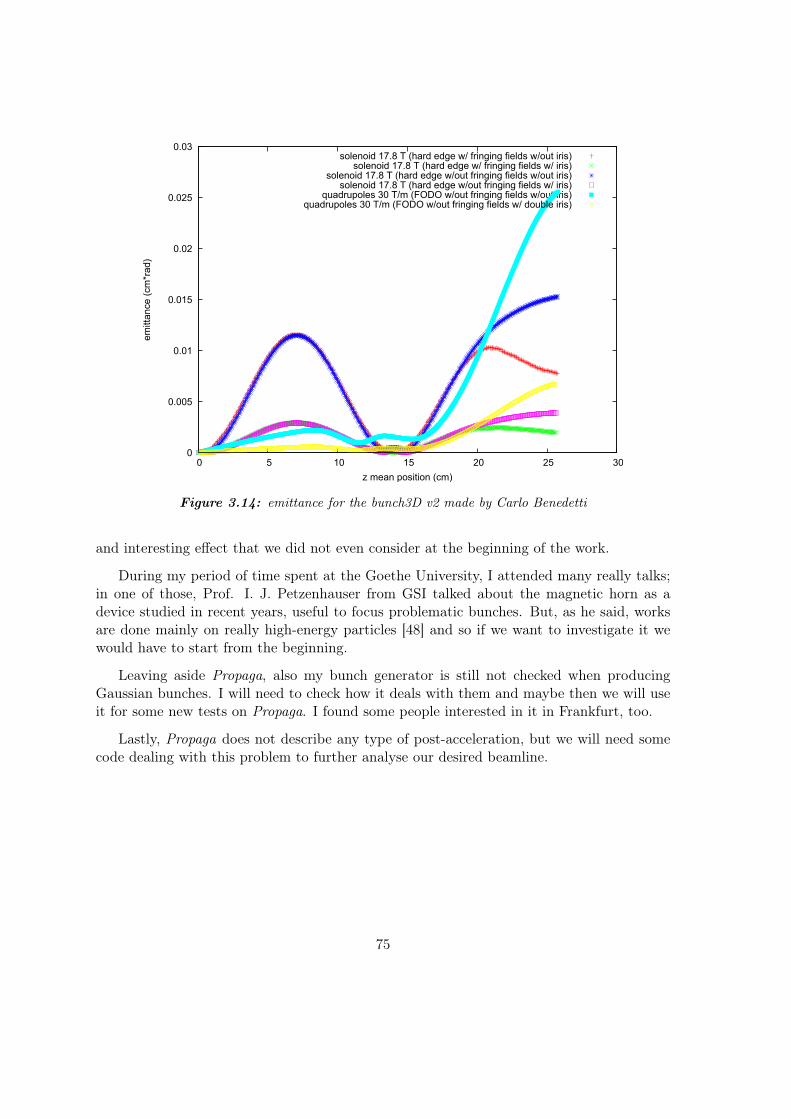
0

0.005

0.01

0.015

0.02

0.025

0.03

0 5 10 15 20 25 30

emitt

ance

(cm

*rad

)

z mean position (cm)

solenoid 17.8 T (hard edge w/ fringing fields w/out iris)solenoid 17.8 T (hard edge w/ fringing fields w/ iris)

solenoid 17.8 T (hard edge w/out fringing fields w/out iris)solenoid 17.8 T (hard edge w/out fringing fields w/ iris)

quadrupoles 30 T/m (FODO w/out fringing fields w/out iris)quadrupoles 30 T/m (FODO w/out fringing fields w/ double iris)

Figure 3.14: emittance for the bunch3D v2 made by Carlo Benedetti

and interesting effect that we did not even consider at the beginning of the work.

During my period of time spent at the Goethe University, I attended many really talks;in one of those, Prof. I. J. Petzenhauser from GSI talked about the magnetic horn as adevice studied in recent years, useful to focus problematic bunches. But, as he said, worksare done mainly on really high-energy particles [48] and so if we want to investigate it wewould have to start from the beginning.

Leaving aside Propaga, also my bunch generator is still not checked when producingGaussian bunches. I will need to check how it deals with them and maybe then we will useit for some new tests on Propaga. I found some people interested in it in Frankfurt, too.

Lastly, Propaga does not describe any type of post-acceleration, but we will need somecode dealing with this problem to further analyse our desired beamline.

75

Figure 3.15: Electron (blue) and proton (cyan to red) flux through the solenoid.The beam has entered the solenoid from the left side of the picture. The electronsare circulating around the axis of the solenoid, leading to a strong negative spacecharge that results in a proton beam focusing and aggregation around the axis too[47].

76

Conclusion

In this thesis I described the work I did in the past year in the framework of the activitiesof the Lilia-INFN experiment at Bologna.

At the moment, here the main research field is the study of laser acceleration of protons.While electron acceleration is known relatively well, protons dynamic treatment, on theother hand, is still under investigation not only here but also in many other theoreticalgroups.

Significant experimental results were obtained only in last years, due to the dramaticimprovements in laser power obtained with the chirped pulse amplification technique. Now,thanks also to the new kinds of targets, it seems that in the near future we will be ca-pable of obtaining protons with energies above one hundred of MeV, sufficient for medicalapplications, such as hadron therapy.

In view of these future possibilities, the group is actively working to simulate the be-haviour of innovative new targets, such as gaseous jet targets, and transport systems. Thepresent work is also focused on the feasibility study of the Prometheus project that aims tocreate a laser based laboratory for the acceleration of protons for biomedical applications incollaboration with ENEA division of Bologna.

In the first chapter of this thesis I analysed the main features of laser-plasma accelerationand the two main laser-proton acceleration regimes. For both of them I described theirdistinctive features and the energies achievable with current technology. These regimes arestudied and simulated here in Bologna with ALaDyn, a particle-in-cell code developed by theBologna’s group itself. My contribution to ALaDyn was the development of algorithms andassociated code to integrate the particle equations of motions using leapfrog and symplecticmethods.

77

In the third chapter I described the main work of my thesis: I studied the problemsof transport of the protons bunches, obtained from laser-plasma interactions. The mainconcern was to limit the growth of emittance with suitable arrangement of focusing devices.This is a key point to couple these bunches with a post-acceleration devices which might beused for cancer treatment.

The first studies on transport system concerned a FODO beamline (focusing-defocusingcoupled quadrupoles). To improve my knowledge on this topic I spent a period of two monthsat the Goethe University in Frankfurt am Main where I collaborated with Prof. Ratzinger’sgroup. Their main activity is the design of new cavities for post-acceleration. There I learntthe importance of solenoids as focusing devices in a beamline; the model we had initiallyconsidered did not include the fringing fields of the solenoid itself. After inserting them, agood agreement with results obtained by the Frankfurt group were obtained.

I also wrote a bunch generator, to simulate a K-V beam, whose propagation was used tomatch with their results. Other simulations were based on bunches obtained from the PICcode ALaDyn.

The results presented here are preliminary even though they show that a laser acceleratedbunch can be transported with a controlled emittance growth. For the future, we plan toinsert the space charge forces and to add the electronic population in our simulations whichhas a focusing effect on protons. A crucial point will be the consideration of different typesof targets which allow to obtain a better bunch for transport.

Stefano Sinigardistefano.sinigardi@gmail.com

78

Bibliography

[1] R. J. Goldston, P. H. Rutherford Introduction to Plasma Physics. IOP, 1995.

[2] J. Chandrashekhar. Plasma Accelerators. Scientific American, February 2006, page40.

[3] G. A. Mourou, T. Tajima, S. V. Bulanov. Optics in the relativistic regime Rev.Mod. Phys., vol. 78, p. 309, April-June 2006

[4] A. Sgattoni Equazioni di Maxwell-Liouville ed accelerazione di cariche tramite unimpulso elettromagnetico. Tesi di Laurea Specialistica in Fisica, A. A. 2005-2006

[5] G. A. Mourou, D. Umstadter. Extreme Light. Scientific American, May 2002.

[6] W. P. Leemans, B. Nagler, A. J. Gonsalves, Cs. Tóth, K. Nakamura, C. G.R. Geddes, E. Esarey, C. B. Schroeder, S. M. Hooker. GeV electron beams froma centimetre-scale accelerator. Nature Physics 2, 696-699 (2006).

[7] W. L. Kruer. The Physics of Laser Plasma Interactions. ABP, 2003.

[8] A. Sgattoni, G. Turchetti, C. Benedetti, P. Londrillo, L. Di Lucchio Compar-ison of scaling laws with PIC simulations for proton acceleration with long wavelengthpulses Nuclear Instruments and Methods in Physics Research Section A, vol. 620 issue1 (2010).

[9] A. Macchi, S. Veghini, F. Pegoraro. Light Sail Acceleration Re-examined. PRL103, 085003, 2009.

[10] C. A. J. Palmer, N. P. Dover, I. Pogorelsky, M. Babzien, G. I. Dudnikova,M. Ispiriyan, M. N. Polyanskiy, J. Schreiber, P. Shkolnikov, V. Yakimenko,

79

Z. Najmudin. Monoenergetic proton beams accelerated by a radiation pressure drivenshock. arXiv:1006.3163v2 [physics.plasm-ph].

[11] A. Macchi, F. Cattani, T. V. Liseykina, F. Cornolti. Laser Acceleration of IonBunches at the Front Surface of Overdense Plasmas. PRL 103, 085003, 2009.

[12] M. Passoni, M. Lontano. One-dimensional model of the electrostatic ion accelerationin the ultraintense laser-solid interaction. Laser and Particle Beams 22, 163-169 (2004).

[13] V. T. Tikhonchuk Interaction of a beam of fast electrons with solids. Physics ofPlasmas 9, n. 4, 1416 (2002).

[14] A. Zani, A. Sgattoni, M. Passoni. Parametric investigations of Target NormalSheath Acceleration Experiments. Preprint submitted to Nuclear Instruments and Meth-ods in Physics - Research Section A, 18 November 2010.

[15] T. Esirkepov, M. Borghesi, S. V. Boulanov, G. Mourou, T. Tajima. HighlyEfficient Relativistic-Ion Generation in the Laser-Piston Regime. Phys. Rev. Lett. 92,175003 (2004).

[16] T. Esirkepov, M. Yamagiwa, T. Tajima Laser Ion-Acceleration Scaling Laws Seenin Multiparametric Particle-in-Cell Simulations. Phys. Rev. Lett. 96, 105001 (2006).

[17] A. Macchi, T. V. Liseykina, S. Tuveri, S. Veghini. Theory and simulation of ionacceleration with circularly polarized laser pulses. C. R. Physique 10 (2009) 207-215

[18] A. Macchi, C. Benedetti. Ion acceleration by radiation pressure in thin and thicktargets. Nucl. Inst. Meth. Phys. Res. A, vol. 620 issue 1 (2010).

[19] F. Cattani, A. Kim, D. Anderson, M. Lisak. Threshold of induced transparencyin the relativistic interaction of an electromagnetic wave with overdense plasmas. Phys.Rev. E 62, 1234-1237 (2000).

[20] A. P. L. Robinson, P. Gibbon, M. Zepf, S. Kar, R. G. Evans, C. Bellei. Rel-ativistically correct hole-boring and ion acceleration by circularly polarized laser pulses.Plasma Phys. Contr. Fusion 51, 024004 (2009).

[21] A. P. L. Robinson et al. Radiation pressure acceleration of thin foils with circularlypolarized laser pulses. New J. Phys. 10 013021 (2008).

[22] T. Schlegel, N. Naumova, V. T. Tikhonchuk, C. Labaune, I. V. Sokolov,G. Mourou. Relativistic laser piston model: Ponderomotive ion acceleration in denseplasmas using ultra-intense laser pulses. Phys. Plasmas 16, 083103 (2009).

[23] G. Turchetti, A. Sgattoni Specchio relativistico ed accelerazione con λ = 10µm.Note personali.

[24] G. Turchetti. Dinamica classica dei sistemi fisici. Zanichelli, 1998.

80

[25] D. Donnelly, E. Rogers. Symplectic integrators: An introduction. Am. J. Phys 73(10), October 2005.

[26] C. K. Birdsall, A. B. Langdon. Plasma physics via computer simulation. IOP, 2005.

[27] M. Schollmeier, S. Becker M. Geißel, K. A. Flippo, A. Blazević, S. A. Gail-lard, D. C. Gautier, F. Grüner, K. Harres, M. Kimmel, F. Nürnberg, P.Rambo, U. Schramm, J. Schreiber, J. Schütrumpf, J. Schwarz, N. A. Tahir,B. Atherton, D. Habs, B. M. Hegelich, M. Roth. Controlled transport and focus-ing of Laser-Accelerated Protons with Miniature Magnetic Devices. PRL 101, 055004,2008.

[28] P. Antici, J. Fuchs, E. d’Humières, J. Robiche, E. Brambrink, S. Atzeni, A.Schiavi, Y. Sentoku, P. Audebert, H. Pépin. Laser acceleration of high-energyprotons in variable density plasmas. New Journal of Physics 11, 023038 (2009).

[29] K. Zeil, S. D. Kraft, S. Bock, M. Bussmann, T. E. Cowan, T. Kluge, J.Metzkes, T. Richter, R. Sauerbrey, U. Schramm. The scaling of proton energiesin ultrashort pulse laser plasma acceleration. New Journal of Physics 12, 045015 (2010).

[30] C. De Martinis. Status of the Lilia Project. Third LIFE Meeting, LNF-INFN (March11-12, 2010)http://lns-lilia.wikispaces.com

[31] G. Turchetti, M. Sumini, P. Londrillo, F. Rocchi , A. Sgattoni, D. Giove,C. De Martinis, L. Serafini, M. Passoni, A. Bacci. Optical acceleration activityin Italy: PlasmonX and Prometheus project. Kyoto, PMRC, Dec. 4th, 2009

[32] M. Sumini. Infrastructures and Roadmap for the Prometheus Project. Kyoto, PMRC,Dec. 4th, 2009.

[33] G. Servizi. Libreria Passe-par-tout.http://www.physycom.unibo.it/labinfo/passe_par_tout.php

[34] R. Tiede et al. LORASR Code Development. Proc. EPAC06, Edinburgh, Scotland(2006).

[35] D. Rusthoi, W. Lysenko, K. Crandall. Further Improvements on Trace-3D. Pro-ceedings of the 1997 Particle Accelerator Conference (Vancouver, May 12-16, 1997).

[36] R. B. Moore. Elliptical Transformations for Beam Optics.

[37] I. M. Kapchinskij, V. V. Vladimirskij. Limitations of proton beam current in astrong focusing linear accelerator associated with the beam space charge. InternationalConference on High-Energy accelerators and instrumentation, 274-288 (CERN, 1959).

81

[38] A. Vivoli, C. Benedetti, G. Turchetti. Time series analysis of Coulomb collisionsin a beam dynamics simulation Nuclear Instruments and Methods in Physics ResearchA 561 (2006) 320-324

[39] K. Flöttmann. Astra. DESY, Hamburg, www.desy.de/~mpyflo, 2000.

[40] K. Flöttmann, S. M. Lidia, P. Piot. Recent Improvements to the ASTRA ParticleTracking Code. Proceedings of PAC03, Oregon, May 2003, pp. 3500-3502.

[41] A. Almomani, M. Droba, U. Ratzinger, I. Hofmann. Matching the laser gener-ated p-bunch into a CH-DTL. Proceedings of IPAC10, Kyoto, Japan (2010).

[42] A. Bazzani, E. Todesco, G. Turchetti, G. Servizi. A normal form approach tothe theory of non-linear betatronic motion. CERN Yellow Report (CERN 94-02), 1994.

[43] H. Wiedemann. Particle Accelerator Physics. Springer, 3rd ed., 2007.

[44] G. Franchetti. Linear Beam optics in solenoidal channels. Phys. Rev. Special Topics- Accelerators and Beams, vol. 4, 074001, 2001.

[45] C. Benedetti, A. Sgattoni, G. Turchetti, P. Londrillo. ALaDyn: A High-Accuracy PIC Code for the Maxwell-Vlasov Equations IEEE Transactions on PlasmaScience, Vol. 36, No. 4, August 2008.

[46] A. Kovalenko, N. Agapov, V. Bartenev, A. Donyagin, I. Eliseeva, H.Khodzhibagiyan, G. Kuznetsov, A. Smirnov, M. Voevodin, E. Fischer, G.Moritz. Design and study of a superferric model dipole and quadrupole magnets for theGSI fast-pulsed synchrotron SIS100. Proceedings of EPAC 2004, Lucerne, Switzerland.

[47] K. Harres, I. Alber, A. Tauschwitz, V. Bagnoud, H. Daido, M. Günther, F.Nürnberg, A. Otten, M. Schollmeier, J. Schütrumpf, M. Tampo, M. Roth.Beam collimation and transport of laser-accelerated protons by a solenoid field. J. Phys.:Conf. Ser. 244, 022036, 2010.

[48] S. Gilardoni, G. Grawer, G. Maire, J. M. Maugain, S. Rangod, F. Voelker.Status of a magnetic horn for a neutrino factory. J. Phys. G: Nucl. Part. Phys. 29,1801-1805 (2003).

82