-sa-asvadi.ir/wp-content/uploads/thesis_alirezaasvadi-compressed.pdf · abstract in this thesis, we...
TRANSCRIPT

Alir
eza
Asv
adi
Mu
lti-S
en
So
r o
bje
ct D
et
ec
tio
n f
or A
ut
on
oM
ou
S D
riv
ing
Alireza Asvadi
Março de 2018
Multi-SenSor object Detection for AutonoMouS Driving
Tese de Doutoramento em Engenharia Electrotécnica e de Computadores, ramo deespecialização em Computadores e Electrónica, orientada pelo Professor Urbano
José Carreira Nunes e Professor Paulo José Monteiro Peixoto e apresentada aoDepartamento de Engenharia Electrotécnica e de Computadores da Faculdade de
Ciências e Tecnologia da Universidade de Coimbra
K Alireza NOVA.indd 1 27/09/2018 12:31:28


Faculty of Science and Technology
Department of Electrical and Computer Engineering
Multi-Sensor Object Detection for Autonomous Driving
Alireza Asvadi
Thesis submitted to the Department of Electrical and Computer Engineering
of the Faculty of Science and Technology of the University of Coimbra in partial fulfillment
of the requirements for the Degree of Doctor of Philosophy
Principal supervisor: Prof. Urbano José Carreira Nunes
Co-supervisor: Prof. Paulo José Monteiro Peixoto
Coimbra
March 2018


Abstract
In this thesis, we propose on-board multisensor obstacle and object detection systemsusing a 3D-LIDAR, a monocular color camera and a GPS-aided Inertial NavigationSystem (INS) positioning data, with application in self-driving road vehicles.
Firstly, an obstacle detection system is proposed that incorporates 4D data (3D spa-tial data and time), and composed by two main modules: (i) a ground surface estimationusing piecewise planes, and (ii) a voxel grid model for static and moving obstacles de-tection using ego-motion information. An extension of the proposed obstacle detectionsystem to a Detection And Tracking Moving Object (DATMO) system is proposed toachieve an object-level perception of dynamic scenes, followed by the fusion of 3D-LIDAR with camera data to improve the tracking function of the DATMO system. Theobstacle detection we propose is to effectively model dynamic driving environment.The proposed DATMO method is able to deal with the localization error of the posi-tion sensing system when computing the motion. The proposed fusion tracking moduleintegrates multiple sensors to improve object tracking.
Secondly, an object detection system based on the hypothesis generation and ver-ification paradigms is proposed using 3D-LIDAR data and Convolutional Neural Net-works (ConvNets). Hypothesis generation is performed by applying clustering on pointcloud data. In the hypothesis verification phase, a depth map is generated using 3D-LIDAR data, and the depth map values are inputted to a ConvNet for object detection.Finally, a multimodal object detection is proposed using a hybrid neural network, com-posed by deep ConvNets and a Multi-Layer Perceptron (MLP) neural network. Threemodalities, depth and reflectance maps (both generated from 3D-LIDAR data) and acolor image, are used as inputs. Three deep ConvNet-based object detectors run indi-vidually on each modality to detect the object bounding boxes. Detections on each oneof the modalities are jointly learned and fused by an MLP-based late-fusion strategy.The purpose of the multimodal detection fusion is to reduce the misdetection rate fromeach modality, which leads to a more accurate detection.
Quantitative and qualitative evaluations were performed using ‘Object DetectionEvaluation’ dataset and ‘Object Tracking Evaluation’ based derived datasets from theKITTI Vision Benchmark Suite. Reported results demonstrate the applicability andefficiency of the proposed obstacle and object detection approaches in urban scenarios.
i

ii
KeywordsAutonomous vehicles; Robotic Perception; Detecting and Tracking of Moving Objects(DATMO); Supervised Learning Based Object Detection

Resumo
Nesta tese e proposto um novo sistema multissensorial de deteccao de obstaculos eobjetos usando um LIDAR-3D, uma camara monocular a cores e um sistema de posi-cionamento baseado em sensores inerciais e GPS, com aplicacao a sistemas de conducaoautonoma.
Em primeiro lugar, propoe-se a criacao de um sistema de detecao de obstaculos,que incorpora dados 4D (3D espacial + tempo) e e composto por dois modulos prin-cipais: (i) uma estimativa do perfil do chao atraves de uma aproximacao planar porpartes e (ii) um modelo baseado numa grelha de voxels para a detecao de obstaculosestaticos e dinamicos recorrendo a informacao do proprio movimento do veıculo. Asfuncionalidade do systemo foram posteriormente aumentado para permitir a Detecao eSeguimento de Objetos Moveis (DATMO) permitindo a percepcao ao nıvel do objetoem cenas dinamicas. De seguida procede-se a fusao dos dados obtidos pelo LIDAR-3D com os dados obtidos por uma camara para melhorar o desempenho da funcao deseguimento do sistema DATMO.
Em segundo lugar, e proposto um sistema de detecao de objetos baseado nos paradig-mas de geracao e verificacao de hipoteses, usando dados obtidos pelo LIDAR-3D, recor-rendo a utilizacao de redes neurais convolucionais (ConvNets). A geracao de hipotesese realizada aplicando um agrupamento de dados ao nıvel da nuvem de pontos. Na fasede verificacao de hipoteses, e gerado um mapa de profundidade a partir dos dados doLIDAR-3D, sendo que esse mapa e inserido numa ConvNet para a detecao de objetos.Finalmente, e proposta uma deteccao multimodal de objetos usando uma rede neuronalhıbrida, composta por Deep ConvNets e uma rede neural do tipo Multi-Layer Perceptron(MLP). As modalidades sensoriais consideradas sao: mapas de profundidade, mapas dereflectancia geradas a partir do LIDAR-3D e imagens a cores. Sao definidos tres dete-tores de objetos que individualmente, em cada modalidade, recorrendo a uma ConvNetdetetam as bounding-boxes do objeto. As detecoes em cada uma das modalidades saodepois consideradas em conjunto e fundidas por uma estrategia de fusao baseada emMLP. O proposito desta fusao e reduzir a taxa de erro na detecao de cada modalidade, oque leva a uma detecao mais precisa.
Foram realizadas avaliacoes quantitativas e qualitativas dos metodos propostos, uti-lizando conjuntos de dados obtidos a partir dos datasets “Avaliacao de Deteccao de
iii

iv
Objetos” e “Avaliacao de Rastreamento de Objetos” do KITTI Vision Benchmark Suite.Os resultados obtidos demonstram a aplicabilidade e a eficiencia da abordagem propostapara a detecao de obstaculos e objetos em cenarios urbanos.
Palavras chaveVeıculos Autonomos; Percepcao Robotica; Deteccao e Seguimento de Objectos Moveis;Detecao de Objectos Baseada em Aprendizagem Supervisionada

Acknowledgment
Foremost, I would like to express my gratitude to my supervisor Prof. Urbano J. Nunesfor his continuous support during my Ph.D. study, and to my co-supervisor Dr. PauloPeixoto for giving me the motivation to achieve more. I also wish to thank Dr. CristianoPremebida for his help and support. I would like to thank co-authors of some papers,specially Pedro Girao, Luis Garrote and Joao Paulo for the discussions and contributionsto enrich my research quality. I would also like to thank my lab colleagues for creating afriendly environment and my Iranian friends who helped me for a fast start in Coimbra.Finally, and on a more personal level, I sincerely thank my family (specially my wifeElham and my parents) for encouraging and supporting me during difficult periods.
I acknowledge the Institute for Systems and Robotics – Coimbra for supportingmy research. This work has been supported by “AUTOCITS - Regulation Study forInteroperability in the Adoption of Autonomous Driving in European Urban Nodes”- Action number 2015-EU-TM-0243-S, co-financed by the European Union (INEA-CEF); and FEDER through COMPETE 2020 program under grants UID/EEA/00048and RECI/EEI-AUT/0181/2012 (AMS-HMI12).
ALIREZA ASVADI
CoimbraMarch 2018
v

vi
c© Copyright by Alireza Asvadi 2018All rights reserved

Contents
1 Introduction 11.1 Context and Motivation . . . . . . . . . . . . . . . . . . . . . . . . . . 21.2 Specific Research Questions and Key Contributions . . . . . . . . . . . 2
1.2.1 Defining the Key Terms . . . . . . . . . . . . . . . . . . . . . 21.2.2 Challenges of Perception for Autonomous Driving . . . . . . . 31.2.3 Summary of Contributions . . . . . . . . . . . . . . . . . . . . 4
1.3 Thesis Outline . . . . . . . . . . . . . . . . . . . . . . . . . . . . . . . 51.3.1 Guidelines for Reading the Thesis . . . . . . . . . . . . . . . . 6
1.4 Publications and Technical Contributions . . . . . . . . . . . . . . . . 71.4.1 Publications . . . . . . . . . . . . . . . . . . . . . . . . . . . . 81.4.2 Software Contributions . . . . . . . . . . . . . . . . . . . . . . 91.4.3 Collaborations . . . . . . . . . . . . . . . . . . . . . . . . . . 9
I BACKGROUND 11
2 Basic Theory and Concepts 132.1 Robot Vision Basics . . . . . . . . . . . . . . . . . . . . . . . . . . . . 13
2.1.1 Sensors for Environment Perception . . . . . . . . . . . . . . . 142.1.2 Sensor Data Representations . . . . . . . . . . . . . . . . . . . 16
Transformation in 3D Space . . . . . . . . . . . . . . . . . . . 172.1.3 Multisensor Data Fusion . . . . . . . . . . . . . . . . . . . . . 20
Sensor Configuration . . . . . . . . . . . . . . . . . . . . . . . 20Fusion Level . . . . . . . . . . . . . . . . . . . . . . . . . . . 21
2.2 Machine Learning Basics . . . . . . . . . . . . . . . . . . . . . . . . . 222.2.1 Supervised Learning . . . . . . . . . . . . . . . . . . . . . . . 22
Multi-Layer Neural Network . . . . . . . . . . . . . . . . . . . 24Convolutional Neural Network . . . . . . . . . . . . . . . . . . 26Optimization . . . . . . . . . . . . . . . . . . . . . . . . . . . 29
2.2.2 Unsupervised Learning . . . . . . . . . . . . . . . . . . . . . . 30DBSCAN . . . . . . . . . . . . . . . . . . . . . . . . . . . . . 31
vii

viii CONTENTS
3 Test Bed Setup and Tools 333.1 The KITTI Vision Benchmark Suite . . . . . . . . . . . . . . . . . . . 33
3.1.1 Sensor Setup . . . . . . . . . . . . . . . . . . . . . . . . . . . 343.1.2 Object Detection and Tracking Datasets . . . . . . . . . . . . . 363.1.3 ‘Object Tracking Evaluation’ Based Derived Datasets . . . . . 36
3.2 Evaluation Metrics . . . . . . . . . . . . . . . . . . . . . . . . . . . . 393.2.1 Average Precision and Precision-Recall Curve . . . . . . . . . 393.2.2 Metrics for Obstacle Detection Evaluation . . . . . . . . . . . . 40
3.3 Packages and Toolkits . . . . . . . . . . . . . . . . . . . . . . . . . . . 413.3.1 YOLOv2 . . . . . . . . . . . . . . . . . . . . . . . . . . . . . 41
4 Obstacle and Object Detection: A Survey 434.1 Obstacle Detection . . . . . . . . . . . . . . . . . . . . . . . . . . . . 44
4.1.1 Environment Representation . . . . . . . . . . . . . . . . . . . 444.1.2 Grid-based Obstacle Detection . . . . . . . . . . . . . . . . . . 45
Ground Surface Estimation . . . . . . . . . . . . . . . . . . . . 46Generic Object Tracking . . . . . . . . . . . . . . . . . . . . . 46Obstacle Detection and DATMO . . . . . . . . . . . . . . . . . 48
4.2 Object Detection . . . . . . . . . . . . . . . . . . . . . . . . . . . . . 504.2.1 Recent Developments in Object Detection . . . . . . . . . . . . 50
Non-ConvNet Approaches . . . . . . . . . . . . . . . . . . . . 50ConvNet based Approaches . . . . . . . . . . . . . . . . . . . 50
4.2.2 Object Detection in ADAS Domain . . . . . . . . . . . . . . . 51Vision-based Object Detection . . . . . . . . . . . . . . . . . . 523D-LIDAR-based Object Detection . . . . . . . . . . . . . . . 523D-LIDAR and Camera Fusion . . . . . . . . . . . . . . . . . 53
II METHODS AND RESULTS 55
5 Obstacle Detection 575.1 Static and Moving Obstacle Detection . . . . . . . . . . . . . . . . . . 58
5.1.1 Static and Moving Obstacle Detection Overview . . . . . . . . 585.1.2 Piecewise Ground Surface Estimation . . . . . . . . . . . . . . 58
Dense Point Cloud Generation . . . . . . . . . . . . . . . . . . 58Piecewise Plane Fitting . . . . . . . . . . . . . . . . . . . . . . 60
5.1.3 Stationary – Moving Obstacle Detection . . . . . . . . . . . . . 64Ground – Obstacle Segmentation . . . . . . . . . . . . . . . . 65Discriminative Stationary – Moving Obstacle Segmentation . . 65
5.2 Extension of Motion Grids to DATMO . . . . . . . . . . . . . . . . . . 695.2.1 2.5D Grid-based DATMO Overview . . . . . . . . . . . . . . . 69
CONTENTS ix
5.2.2 From Motion Grids to DATMO . . . . . . . . . . . . . . . . . 692.5D Motion Grid Detection . . . . . . . . . . . . . . . . . . . 70Moving Object Detection and Tracking . . . . . . . . . . . . . 72
5.3 Fusion at Tracking-Level . . . . . . . . . . . . . . . . . . . . . . . . . 745.3.1 Fusion Tracking Overview . . . . . . . . . . . . . . . . . . . . 745.3.2 3D Object Localization in PCD . . . . . . . . . . . . . . . . . 755.3.3 2D Object Localization in Image . . . . . . . . . . . . . . . . 785.3.4 KF-based 2D/3D Fusion and Tracking . . . . . . . . . . . . . . 80
6 Object Detection 836.1 3D-LIDAR-based Object Detection . . . . . . . . . . . . . . . . . . . 84
6.1.1 DepthCN Overview . . . . . . . . . . . . . . . . . . . . . . . . 846.1.2 HG Using 3D Point Cloud Data . . . . . . . . . . . . . . . . . 84
Grid-based Ground Removal . . . . . . . . . . . . . . . . . . . 84Obstacle Segmentation for HG . . . . . . . . . . . . . . . . . . 85
6.1.3 HV Using DM and ConvNet . . . . . . . . . . . . . . . . . . . 86DM Generation . . . . . . . . . . . . . . . . . . . . . . . . . . 86ConvNet for Hypothesis Verification (HV) . . . . . . . . . . . 89
6.1.4 DepthCN Optimization . . . . . . . . . . . . . . . . . . . . . . 90HG Optimization . . . . . . . . . . . . . . . . . . . . . . . . . 90ConvNet Training using Augmented DM Data . . . . . . . . . 90
6.2 Multimodal Object Detection . . . . . . . . . . . . . . . . . . . . . . 906.2.1 Fusion Detection Overview . . . . . . . . . . . . . . . . . . . 916.2.2 Multimodal Data Generation . . . . . . . . . . . . . . . . . . . 926.2.3 Vehicle Detection in Modalities . . . . . . . . . . . . . . . . . 926.2.4 Multimodal Detection Fusion . . . . . . . . . . . . . . . . . . 92
Joint Re-Scoring using MLP Network . . . . . . . . . . . . . . 93Non-Maximum Suppression . . . . . . . . . . . . . . . . . . . 94
7 Experimental Results and Discussion 977.1 Obstacle Detection Evaluation . . . . . . . . . . . . . . . . . . . . . . 97
7.1.1 Static and Moving Obstacle Detection . . . . . . . . . . . . . . 97Evaluation of Ground Estimation . . . . . . . . . . . . . . . . 99Evaluation of Stationary – Moving Obstacle Detection . . . . . 99Computational Analysis . . . . . . . . . . . . . . . . . . . . . 101Qualitative Results . . . . . . . . . . . . . . . . . . . . . . . . 102Extension to DATMO . . . . . . . . . . . . . . . . . . . . . . 105
7.1.2 Multisensor Generic Object Tracking . . . . . . . . . . . . . . 106Evaluation of Position Estimation . . . . . . . . . . . . . . . . 107Evaluation of Orientation Estimation . . . . . . . . . . . . . . 107Computational Analysis . . . . . . . . . . . . . . . . . . . . . 108

x CONTENTS
Qualitative Results . . . . . . . . . . . . . . . . . . . . . . . . 1087.2 Object Detection Evaluation . . . . . . . . . . . . . . . . . . . . . . . 111
7.2.1 3D-LIDAR-based Detection . . . . . . . . . . . . . . . . . . . 111Evaluation of Recognition . . . . . . . . . . . . . . . . . . . . 112Evaluation of Detection . . . . . . . . . . . . . . . . . . . . . 112Computational Analysis . . . . . . . . . . . . . . . . . . . . . 112Qualitative Results . . . . . . . . . . . . . . . . . . . . . . . . 113
7.2.2 Multimodal Detection Fusion . . . . . . . . . . . . . . . . . . 113Evaluation on Validation Set . . . . . . . . . . . . . . . . . . . 115Evaluation on KITTI Online Benchmark . . . . . . . . . . . . 119Computational Analysis . . . . . . . . . . . . . . . . . . . . . 120Qualitative Results . . . . . . . . . . . . . . . . . . . . . . . . 122
III CONCLUSIONS 123
8 Concluding Remarks and Future Directions 1258.1 Summary of Thesis Contributions . . . . . . . . . . . . . . . . . . . . 125
8.1.1 Obstacle Detection . . . . . . . . . . . . . . . . . . . . . . . . 1258.1.2 Object Detection . . . . . . . . . . . . . . . . . . . . . . . . . 126
8.2 Discussions and Future Perspectives . . . . . . . . . . . . . . . . . . . 127
Appendices
Appendix A 3D Multisensor Single-Object Tracking Benchmark 131A.1 Baseline 3D Object Tracking Algorithms . . . . . . . . . . . . . . . . 132A.2 Quantitative Evaluation Methodology . . . . . . . . . . . . . . . . . . 134A.3 Evaluation Results and Analysis of Metrics . . . . . . . . . . . . . . . 135
A.3.1 A Comparison of Baseline Trackers with the State-of-the-artComputer Vision based Object Trackers . . . . . . . . . . . . . 136
Appendix B Object Detection Using Reflection Data 139B.1 Computational Complexity and Run-Time . . . . . . . . . . . . . . . . 140B.2 Quantitative Results . . . . . . . . . . . . . . . . . . . . . . . . . . . . 140
B.2.1 Sparse Reflectance Map vs RM . . . . . . . . . . . . . . . . . 140B.2.2 RM Generation Using Nearest Neighbor, Linear and Natural
Interpolations . . . . . . . . . . . . . . . . . . . . . . . . . . . 141B.3 Qualitative Results . . . . . . . . . . . . . . . . . . . . . . . . . . . . 142
Bibliography 145
List of Figures
1.1 The summary of contributions. . . . . . . . . . . . . . . . . . . . . . . 51.2 An illustrative block diagram of the contents of Chapters 5 and 6. . . . . 7
2.1 A summary of advancement of 3D-LIDAR technologies. . . . . . . . . 152.2 Employed data representations. . . . . . . . . . . . . . . . . . . . . . . 162.3 Coordinate frames and relative poses. . . . . . . . . . . . . . . . . . . 192.4 A symbolic representation of Durrant-Whyte’s data fusion schemes. . . 202.5 An example of single hidden layer MLP. . . . . . . . . . . . . . . . . . 252.6 ConvNet layers. . . . . . . . . . . . . . . . . . . . . . . . . . . . . . . 282.7 Basic architecture of ConvNet. . . . . . . . . . . . . . . . . . . . . . . 292.8 Main concepts in DBSCAN. . . . . . . . . . . . . . . . . . . . . . . . 31
3.1 Sensors setup on AnnieWAY. . . . . . . . . . . . . . . . . . . . . . . . 343.2 The top view of the multisensor configuration. . . . . . . . . . . . . . . 353.3 An example of the stationary and moving obstacle detection’s GT data. . 38
4.1 Some approaches for the appearance modeling of a target object. . . . . 47
5.1 Architecture of the proposed obstacle detection system. . . . . . . . . . 595.2 An example of the generated dense PCD. . . . . . . . . . . . . . . . . 605.3 Illustration of the variable-size ground slicing. . . . . . . . . . . . . . . 615.4 An example of the application of the gating strategy on a dense PCD. . 625.5 The piecewise RANSAC plane fitting process. . . . . . . . . . . . . . . 635.6 Binary mask generation for the stationary and moving voxels. . . . . . . 665.7 An example result of the proposed obstacle detection system. . . . . . . 685.8 The architecture of the 2.5D grid-based DATMO algorithm. . . . . . . . 695.9 The motion computation process. . . . . . . . . . . . . . . . . . . . . . 715.10 The 2.5D grid-based motion detection process. . . . . . . . . . . . . . 725.11 A sample screenshot of the proposed 2.5D DATMO result. . . . . . . . 735.12 Pipeline of the proposed fusion-based object tracking algorithm. . . . . 755.13 Proposed object tracking method results. . . . . . . . . . . . . . . . . . 765.14 The ground removal process. . . . . . . . . . . . . . . . . . . . . . . . 77
xi

xii LIST OF FIGURES
5.15 The MS procedure in the PCD. . . . . . . . . . . . . . . . . . . . . . . 785.16 The MS computation in the image. . . . . . . . . . . . . . . . . . . . . 79
6.1 The proposed 3D-LIDAR-based vehicle detection algorithm (DepthCN). 856.2 HG using DBSCAN in a given point cloud. . . . . . . . . . . . . . . . 866.3 The generated dense-Depth Map (DM) with the projected hypotheses. . 876.4 Illustration of the DM generation process. . . . . . . . . . . . . . . . . 886.5 The ConvNet architecture. . . . . . . . . . . . . . . . . . . . . . . . . 896.6 The pipeline of the proposed multimodal vehicle detection algorithm. . 916.7 Feature extraction and the joint re-scoring training strategy. . . . . . . . 936.8 Illustration of the fusion detection process. . . . . . . . . . . . . . . . . 95
7.1 Evaluation of the proposed ground estimation algorithm. . . . . . . . . 987.2 An example of the obstacle detection evaluation. . . . . . . . . . . . . 1007.3 Computational analysis of the proposed obstacle detection method. . . . 1027.4 A few frames of obstacle detection results (sequences 1 to 4). . . . . . . 1037.5 A few frames of obstacle detection results (sequences 5 to 8). . . . . . . 1047.6 2.5D grid-based DATMO results of 3 typical sequences. . . . . . . . . . 1067.7 Object tracking results (sequences 1 to 4). . . . . . . . . . . . . . . . . 1097.8 Object tracking results (sequences 5 to 8). . . . . . . . . . . . . . . . . 1107.9 The precision-recall of the proposed DepthCN method on KITTI. . . . . 1137.10 Few examples of DepthCN detection results. . . . . . . . . . . . . . . . 1147.11 The vehicle detection performance in color, DM and RM modalities. . . 1167.12 The joint re-scoring function learned from the confidence score. . . . . 1177.13 Influence of the number of layers / hidden neurons on MLP performance. 1187.14 Multimodal fusion vehicle detection performance. . . . . . . . . . . . . 1197.15 The precision-recall of the multimodal fusion detection on KITTI. . . . 1207.16 Fusion detection system results. . . . . . . . . . . . . . . . . . . . . . 1217.17 The parallelism architecture for real-time implementation. . . . . . . . 122
A.1 The precision plot of 3D overlap rate. . . . . . . . . . . . . . . . . . . 135A.2 The precision plot of orientation error. . . . . . . . . . . . . . . . . . . 136A.3 The precision plot of location error. . . . . . . . . . . . . . . . . . . . 137
B.1 Precision-Recall using sparse RM vs RM. . . . . . . . . . . . . . . . . 141B.2 Precision-Recall using RM with different interpolation methods. . . . . 142B.3 An example of color image, RMnearest, RMnatural and RMlinear. . . . . . 143B.4 Examples of RefCN results. . . . . . . . . . . . . . . . . . . . . . . . 144
List of Tables
3.1 Detailed information about each sequence used for the stationary andmoving obstacle detection evaluation. . . . . . . . . . . . . . . . . . . 37
3.2 Detailed information about each sequence used for multisensor 3D single-object tracking evaluation. . . . . . . . . . . . . . . . . . . . . . . . . 39
4.1 Comparison of some major grid-based environment representations. . . 454.2 Some of the recent obstacle detection and tracking methods for au-
tonomous driving applications. . . . . . . . . . . . . . . . . . . . . . . 494.3 Related work on 3D-LIDAR-based object detection. . . . . . . . . . . . 534.4 Some recent related work on 3D-LIDAR and camera fusion. . . . . . . 54
7.1 Values considered for the main parameters used in the proposed obstacledetection algorithm. . . . . . . . . . . . . . . . . . . . . . . . . . . . . 98
7.2 Results of the evaluation of the proposed obstacle detection algorithm. . 1007.3 Percentages of the computational load of the different steps of the pro-
posed system. . . . . . . . . . . . . . . . . . . . . . . . . . . . . . . . 1017.4 Values considered for the main parameters used in the proposed 2.5D
grid-based DATMO algorithm. . . . . . . . . . . . . . . . . . . . . . . 1057.5 Values considered for the main parameters used in the proposed 3D fu-
sion tracking algorithm. . . . . . . . . . . . . . . . . . . . . . . . . . . 1077.6 Average object’s center position errors in 2D (pixels) and 3D (meters). . 1087.7 Orientation estimation evaluation (in radian) . . . . . . . . . . . . . . . 1087.8 The ConvNet’s vehicle recognition accuracy with (W) and without (WO)
applying data augmentation (DA). . . . . . . . . . . . . . . . . . . . . 1127.9 DepthCN vehicle detection evaluation (given in terms of average preci-
sion) on KITTI test-set. . . . . . . . . . . . . . . . . . . . . . . . . . . 1127.10 Evaluation of the studied vehicle detectors on the KITTI Dataset. . . . . 1197.11 Fusion Detection Performance on KITTI Online Benchmark. . . . . . . 120
A.1 Detailed information and challenging factors for each sequence. . . . . 133
B.1 The RefCN processing time (in milliseconds). . . . . . . . . . . . . . . 140
xiii

xiv LIST OF TABLES
B.2 Detection accuracy with sparse RM vs RM on validation-set. . . . . . . 141B.3 Detection accuracy using RM with different interpolation methods on
validation-set. . . . . . . . . . . . . . . . . . . . . . . . . . . . . . . . 142

List of Algorithms
1 The DBSCAN algorithm [1]. . . . . . . . . . . . . . . . . . . . . . . . 322 Dense Point Cloud Generation. . . . . . . . . . . . . . . . . . . . . . . 593 Piecewise Ground Surface Estimation. . . . . . . . . . . . . . . . . . . 644 Short-Term Map Update. . . . . . . . . . . . . . . . . . . . . . . . . . 70
xv

xvi LIST OF ALGORITHMS

List of Abbreviations
1D One-Dimensional; One-Dimension
2D Two-Dimensional; Two-Dimensions
3D Three-Dimensional; Three-Dimensions
4D Four-Dimensional; Four-Dimensions
ADAS Advanced Driver Assistance Systems
AI Artificial Intelligence
ANN Artificial Neural Network
AP Average Precision
AV Autonomous Vehicle
BB Bounding Box
BOF Bayesian Occupancy Filter
BoW Bag of Words
BP Back Propagation
CAD Computer Aided Design
CA-KF Constant Acceleration Kalman Filter
CNN Convolutional Neural Network
ConvNet Convolutional Neural Network
CPU Central processing unit
CV-KF Constant Velocity Kalman Filter
xvii

xviii LIST OF ALGORITHMS
CUDA Compute Unified Device Architecture
DATMO Detection And Tracking Moving Object
DBSCAN Density-Based Spatial Clustering of Applications with Noise
DEM Digital Elevation Map
DM (dense) Depth Map
DoF Degrees of Freedom
DPM Deformable Part Model
DT Delaunay Triangulation
EKF Extended Kalman Filter
FC Fully-Connected
FCN Fully Convolutional Network
FCTA Fast Clustering and Tracking Algorithm
FoV Field of View
fps frames per second
GD Gradient Descent
GNN Global Nearest Neighborhood
GNSS Global Navigation Satellite System
GPS Global Positioning System
GPU Graphical Processing Unit
GT Ground-Truth
HG Hypothesis Generation
HHA Horizontal disparity, Height and Angle feature maps
HOG Histogram of Oriented Gradients
HV Hypothesis Verification

LIST OF ALGORITHMS xix
ICP Iterative Closest Point
IMU Inertial Measurement Unit
INS Inertial Navigation System
IOU Intersection Over Union
ITS Intelligent Transportation System
IV Intelligent Vehicle
KDE Kernel Density Estimation
KF Kalman Filter
LBP Local Binary Patterns
LIDAR LIght Detection And Ranging
LLR Log-Likelihood Ratio
LS Least Square
MB-GD Mini-Batch Gradient Descent
mDE mean of Displacement Errors
MHT Multiple Hypothesis Tracking
MLP Multi-Layer Perceptron
MLS Multi-Level Surface map
MS Mean-Shift
MSE Mean Squared Error
NMS Non-Maximal Suppression
NN Nearest Neighbor; Neural Network
PASCAL VOC The PASCAL Visual Object Classes project
PCD Point Cloud Data
PF Particle Filter
xx LIST OF ALGORITHMS
PDF Probability Density Function
PR Precision-Recall
R-CNN Region-based ConvNet
RADAR RAdio Detection and Ranging
RANSAC RANdom SAmple Consensus
ReLU Rectified Linear Unit
RGB Red Green Blue
RGB-D Red Blue Green and Depth
RM (dense) Reflection Map
ROI Region Of Interest
RPN Region Proposal Network
RTK Real Time Kinematic
sDM sparse Depth Map
SGD Stochastic Gradient Descent
Sig. Sigmoid
SIFT Scale-Invariant Feature Transform
SLAM Simultaneous Localization And Mapping
SPPnets Spatial Pyramid Pooling networks
sRM sparse Range Map; sparse Reflectance Map
SS Selective Search
SSD Single Shot Detector
SVD Singular Value Decomposition
SVM Support Vector Machine
YOLO You Only Look Once real-time object detection system

List of Symbols and Notations
Symbols
7→ maps to← assignment. set/0 empty set⊂ subset∈ belonging to a set≈ approximation‖.‖ Euclidean norm∩ intersections of sets∪ union of sets∧ logical and∨ logical or∂ partial derivative∆ difference between two variablesb.c floor function, truncation operation⊕ dilation (morphology) operationR set of real numbers
General Notation and Indexing
i first-order index i ∈ 1, . . . ,Nj second-order index j ∈ 1, . . . ,Ma scalars, vectorsai i-th element of vector aA matricesA> transpose of matrix AA−1 inverse of matrix A|A| determinant of matrix AA sets
xxi

xxii LIST OF ALGORITHMS
Sensor Data
P a LIDAR PCDx,y,z,r LIDAR data (3D real-value spatial data and 8-bit reflection intensity)µ height value in a grid cellE Elevation gridS local (static) short-term mapM 2.5D motion gridc occupancy valueυ voxel sizeu,v size parameters of an imaged 8-bit depth-value in a depth map
Transformations and Projections
R rotation matrixt translation vectorT transformation matrixT transformation in homogeneous coordinatesPC2I camera coordinate system to image plane projection matrixR0 rectification matrixPL2C LIDAR to camera coordinate system projection matrixϕ,θ ,ψ Euler angles roll, pitch and yaw
Machine Learning
D unknown data distributionD independently and identically distributed (i.i.d.) datax(i),y(i) i-th pair of labeled training exampleh learned mappingL loss functionR regularization functionJ loss function with regularizationθ parameters to learnW,b weight matrix and bias parameters of a neural networkF (·) activation functionLi i-th layer of MLP neural networknl number of layers in MLPW a 2D weighting kernelS feature mapk number of kernelsw,h kernel width and height
LIST OF ALGORITHMS xxiii
z zero paddings strideα learning ratec cluster label
Miscellaneous Notation
∆α angle between LIDAR scans (in elevation direction)η a constant that determines number of intervals to compute slice sizesλi edge of i-th sliceai,bi,ci,di parameters of i-th planeni unit normal vector of i-th planeδZ distance between two consecutive planesδψ angle between two consecutive planesCs,Cd static and dynamic countersBs,Bd static and dynamic binary masksR LLRKσ (.) Gaussian kernel with width σ
Θ set of 1D angle valuesχ center of 3D-BBµ(.) mean functionℜ color model of an objectΩ 2D convex-hullf confidence map

xxiv LIST OF ALGORITHMS

Chapter 1
Introduction
Contents1.1 Context and Motivation . . . . . . . . . . . . . . . . . . . . . . . . 2
1.2 Specific Research Questions and Key Contributions . . . . . . . . 2
1.2.1 Defining the Key Terms . . . . . . . . . . . . . . . . . . . . 2
1.2.2 Challenges of Perception for Autonomous Driving . . . . . . 3
1.2.3 Summary of Contributions . . . . . . . . . . . . . . . . . . . 4
1.3 Thesis Outline . . . . . . . . . . . . . . . . . . . . . . . . . . . . . 5
1.3.1 Guidelines for Reading the Thesis . . . . . . . . . . . . . . . 6
1.4 Publications and Technical Contributions . . . . . . . . . . . . . . 7
1.4.1 Publications . . . . . . . . . . . . . . . . . . . . . . . . . . . 8
1.4.2 Software Contributions . . . . . . . . . . . . . . . . . . . . . 9
1.4.3 Collaborations . . . . . . . . . . . . . . . . . . . . . . . . . 9
Science is nothing but perception.
Plato
This chapter describes the context, motivation and aims of the study, and summariesthe study rationale. Then, the organization of the thesis and overview of the chaptersare presented. The last section of this chapter describes the dissemination, softwarecomponents and collaborations.
1

2 CHAPTER 1. INTRODUCTION
1.1 Context and MotivationInjuries caused by motorized road transport was the eighth-leading cause of death world-wide with over 1.3 million deaths in 2010 [2]. By 2020, it is predicted that road acci-dents will take the lives of around 1.9 million people [3]. Studies show that human erroraccounts for more than 94% of accidents [4]. In order to reduce the unacceptably highnumber of death and road injuries resulting from human error, researchers are trying toshift the paradigm of the transportation system, in which the task of a driver changesfrom driving to supervising the vehicle. Autonomous Vehicles (AV) which are able toperceive environment and take appropriate actions can expected to be a viable solutionto the aforementioned problem.
In the last couple of decades, autonomous driving and Advanced Driver AssistanceSystems (ADAS) have had remarkable progress. The perception systems of ADASs andAVs, which is of interest here, perceives the environment and builds an internal modelof the environment using sensor data. In most cases, AVs [5, 6] are equipped with avaried set of on board sensors e.g., mono and stereo cameras, LIDAR and Radar to havea multimodal, redundant and robust perception of the driving scene. Among the above-named sensors, 3D-LIDARs are the pivotal sensing solution for ensuring the high-levelof reliability and safety demanded for autonomous driving systems. In this thesis, wepropose a framework for driving environment perception with the fusion of 3D-LIDAR,monocular color camera and GPS-aided Inertial Navigation System (INS) data. Thespecific research questions and the main contributions of this thesis are addressed in thenext sections.
1.2 Specific Research Questions and Key ContributionsDespite the impressive progress already accomplished in modeling and perceiving thesurrounding environment of AVs, incorporating multisensor multimodal data and de-signing a robust and accurate obstacle and object detection system is still a very chal-lenging task, which we are trying to address in this thesis. Some of the commonlyused terms in the proposed approach, key issues for driving scene understanding, and asummary of the contributions are provided in the following sections.
1.2.1 Defining the Key TermsIn this section we define the key terms that refer to the concepts at the core of this thesis.
• Obstacle detection. Throughout this dissertation, the terms ‘Obstacle’ and ‘genericobject’ are used interchangeably to refer to anything that stands on the ground(usually on the road in the vicinity of the AV), which can potentially lead to a

1.2. SPECIFIC RESEARCH QUESTIONS AND KEY CONTRIBUTIONS 3
collision and obstructs the AV’s mission. Examples of obstacles are items likeas traffic signal poles, street trees, fireplugs, objects (e.g., pedestrians, cars andcyclists), animals, rocks, etc. Obstacles can be items that are foreign to usualdriving environment like as auto parts or waste/trash which may have been delib-erately or accidentally left on the road. The term ‘obstacle detection’ will referto using sensor data to detect and localize all entities (obstacles) over the ground.From the practical point of view, obstacle detection is closely coupled with thefree-space detection and has a direct application in safe driving systems such ascollision detection and avoidance systems.
• (Class-specific) object detection. The term ‘object detection’ will be used inthis thesis to refer to discovery of specific categories of objects (e.g., pedestri-ans, cars and cyclists) within a driving scene from sensor data. Class-specificobject detection closely corresponds to the supervised learning paradigm, whereGround-Truth (GT) training labels are available (please refer to section 2.2.1 formore details). The term ‘3D object detection’ will be used in this study to describethe identification of the volume of specific class of objects from the sensor dataor a ‘Representation’ of the sensor data in R3. The term ‘representation’ is usedto describe the encoding of sensor data into a form suitable for computationalprocessing. To see more about sensor data representations please refer to section2.1.2. It should be noted that the detection of the angular position, orientation orpose of the object is not addressed in this thesis.
1.2.2 Challenges of Perception for Autonomous Driving
Autonomous driving has seen a lot of progress recently, however, to increase AVs ca-pability to perform with high reliability in dynamic (real-world) driving conditions, theperception system of AVs need to be empowered with a stronger representation and agreater understanding of their surroundings. In summary, the following key problemsfor perceiving the dynamic road scene were deduced.
• Question 1. What is an effective representation of the dynamic driving scene?How to efficiently and effectively segment the static and moving parts (obstacles)of the driving scene? How to detect generic moving objects and deal with thelocalization error in the AV’s position sensing?
• Question 2. On what level should multisensor fusion act? How to integrate mul-tiple sources of sensor data to reliably perform object tracking? How to build areal-time multisensor multimodal object detection system, and how to overcomelimitations in each sensor/modality?

4 CHAPTER 1. INTRODUCTION
1.2.3 Summary of ContributionsThe key contributions of this thesis are novel approaches for multisensor obstacle andobject detection. To summarize, the following specific contributions were proposed:
• A Stationary and Moving Obstacle Segmentation System. To address the ques-tion of “what is an effective representation of the dynamic driving scene?, andhow to efficiently segment the static and moving parts (obstacles) of the drivingscene?”, we proposed an approach for modeling the 3D dynamic driving scene us-ing a set of variable-size planes and arrays of voxels. 3D-LIDAR and GPS-aidedInertial Navigation System (INS) data are used as inputs. The set of variable-size planes are used to estimate and model non-planar grounds, such as undulatedroads and curved uphill - downhill ground surfaces. The voxel pattern represen-tation is used to effectively model obstacles, which are further segmented into:static obstacles and moving obstacles (see Fig. 1.1 (a)).
• A Generic Moving Object Detection System. In an attempt to address the prob-lem “how to detect generic moving objects and deal with the localization error inthe AV’s position sensing?”, we proposed a motion detection mechanism that canhandle localization errors and suppress false detections using spatial reasoning.The proposed method extracts an object-level representation from motion grids,in the absence of a priori assumption on the shape of objects, which makes itsuitable for a wide range of objects (see Fig. 1.1 (b)).
• A Multisensor Generic Object Tracking System. In an attempt to answer thequestion, “on what level should multisensor fusion act to reliably perform ob-ject tracking?”, we proposed a multisensor 3D object tracking system which isdesigned to maximize the benefits of using dense color images and sparse 3D-LIDAR point-clouds in combination with INS localization data. Two parallelmean-shift algorithms are applied for object detection and localization in the 2Dimage and 3D point-cloud, followed by a robust 2D/3D Kalman Filter (KF) basedfusion and tracking (see Fig. 1.1 (c)).
• A Multimodal Object Detection System. Ultimately, with the aim to answerthe question “how to build a real-time multisensor multimodal object detectionsystem, and how to overcome limitations in each sensor/modality?”, we pro-posed an approach using a hybrid neural network, composed of a ConvNet anda Multi-Layer Perceptron (MLP), to combine front-view dense maps generatedfrom range and reflection intensity modalities from 3D-LIDAR with color cam-era, in a decision-level fusion framework. The proposed approach is trained tolearn and model the nonlinear relationships among modalities, and to deal withdetection limitations in each modality (see Fig. 1.1 (d)).

1.3. THESIS OUTLINE 5
Figure 1.1: The summary of contributions. (a) a stationary and moving obstacle seg-mentation system using 3D-LIDAR and INS data, where the ground surface is shownin blue, static obstacles are shown in red, and moving obstacles are depicted in green,(b) a generic moving object detection system using 3D-LIDAR and INS data, where thedetected generic moving objects are indicated in green bounding boxes, (c) a multisen-sor generic object tracking system using 3D-LIDAR, camera and INS data, where thetracked generic object is shown in green, and (d) a multimodal object detection system,where the detected object categories are demonstrated in different colors.
1.3 Thesis OutlineThis introductory chapter gave the general context of this thesis, contributions and struc-ture of the thesis. The outline of remaining chapters is presented as following.
Part I – BACKGROUND
Chapter 2 – Basic Theory and ConceptsIn this chapter we describe the related concepts, theoretical and mathematical back-grounds required for developing the proposed approaches. Some ideas of Robot Vi-sion, such as sensor data representation and multisensor data fusion are described.Then, a brief introduction of Machine Learning with a focus on supervised andunsupervised learning paradigms is presented.Chapter 3 – Test Bed Setup and ToolsThis chapter introduces the reader to the experimental setup, the dataset and theevaluation metrics. We discuss also the packages and libraries that we have used todevelop our approach.Chapter 4 – Obstacle and Object Detection: A SurveyIn this chapter, we will give an overview of approaches for obstacle and object de-tection. More specifically, the survey focuses on the current state-of-the-art fordynamic driving environment representation, obstacle detection and recent devel-opments in object detection in ADAS domain.

6 CHAPTER 1. INTRODUCTION
Part II – METHODS AND RESULTS
Chapter 5 – Obstacle DetectionThis chapter addresses the problem of obstacle detection in dynamic urban environ-ments. First we propose a complete framework for 3D static and moving obstaclesegmentation and ground surface estimation using voxel pattern representation andpiecewise planes. Next, we discuss on generic moving object detection while con-sidering errors in positioning data. Finally, we propose a multisensor system archi-tecture for the fusion of 3D-LIDAR, color camera and Inertial Navigation System(INS) data at tracking-level.Chapter 6 – Object DetectionThis chapter addresses the problem of object detection. First we start by introduc-ing a 3D object detection system based on the Hypothesis Generation (HG) andVerification (HV) paradigms using only 3D-LIDAR data. Next, we propose an ex-tended approach for real-time multisensor and multimodal object detection withfusion of 3D-LIDAR and camera data. Three modalities, RGB image from colorcamera, front view dense (up-sampled) representations of 3D-LIDAR’s range andreflectance data are used as inputs to a hybrid neural network, which consists of aConvNet and a Multi-Layer Perceptron (MLP), to achieve object detection.Chapter 7 – Results and DiscussionIn this chapter, we will analysis the results of our work. The experiments focus onthe evaluation of the proposed obstacle detection and object detection approaches.A comparison with the state-of-the-art methods and the discussion about the ob-tained results are provided.
Part III – CONCLUSIONS
Chapter 8 – Concluding Remarks and Future DirectionsThe chapter concludes the thesis with discussions on the thesis novelty, contribu-tions, the achieved objectives, and also suggestions for future works.
1.3.1 Guidelines for Reading the ThesisThis section provides guidelines for reading this thesis and explains how different partsof the thesis are related to each other and gives suggestions for reading order. As intro-duced in this chapter, the main novelty of this research is a multisensor framework forobstacle detection and object detection for autonomous driving. A familiarity with thebasic concepts and related works are helpful, though we present the relevant preliminar-ies in the first part of the thesis. Readers that are familiar with those topics may wishto skip Part I. The second part is mainly based on the 9 published papers (see section

1.4. PUBLICATIONS AND TECHNICAL CONTRIBUTIONS 7
1.4.1), which comprises the main body of this thesis and presents the contributions andresults. For the sake of clarity and in order to improve the thesis readability, Part IIfollows mostly the course of the developed work itself (chronological order). Chapters5 and 6, which describe our obstacle and object detection approaches, could be readseparately (see Fig. 1.2). The reader interested in processing of temporal sequence ofmultisensor data may focus particularly on Chapter 5. In this chapter we describe theproposed stationary and moving obstacle segmentation, and generic moving object de-tection and tracking. A reader who is mostly interested in multisensor category-basedobject detection from a single frame of sensors’ data, which is related to supervisedlearning paradigm, may want to focus on Chapter 6. In this chapter we describe 3D-LIDAR-based and multimodal object detection systems. Chapter 7 presents the experi-mental results and analysis. Finally, in Part III, the reader can find conclusions and oursuggestions for future directions.
Chapter 6: Object Detection
3D-LIDAR-basedObject Detection
Multimodal Object Detection
Fusion at Tracking-Level
Chapter 5: Obstacle Detection
Generic Moving Object Detection
Static and Moving Obstacle Segmentation
3D-LIDAR
RGB Camera
INS (GPS/IMU)
Figure 1.2: An illustrative block diagram of the contents of Chapters 5 and 6. Thesensors used for each algorithm are shown in the bottom part of the figure.
1.4 Publications and Technical Contributions
Some preliminary reports of the findings and intermediate results of this thesis havebeen published in 9 papers. Moreover, implementation of the proposed approach led tothe development of a set of software modules/toolboxes, some of them with the collab-oration of other colleagues.

8 CHAPTER 1. INTRODUCTION
1.4.1 PublicationsThe core parts of this thesis is based on the following peer-reviewed publications of theauthor.
Journal Publications
• A. Asvadi, L. Garrote, C. Premebida, P. Peixoto, U. Nunes, Multimodal VehicleDetection: Fusing 3D-LIDAR and color camera data, Pattern Recognition Letters,Elsevier, 2017. DOI: 10.1016/j.patrec.2017.09.038
• A. Asvadi, C. Premebida, P. Peixoto, and U. Nunes, 3D-LIDAR-based Staticand Moving Obstacle Detection in Driving Environments: An approach basedon voxels and multi-region ground planes, Robotics and Autonomous Systems,Elsevier, vol. 83, pp. 299-311, 2016. DOI: 10.1016/j.robot.2016.06.007
Conference Proceedings and Workshops
• A. Asvadi, L. Garrote, C. Premebida, P. Peixoto, U. Nunes, Real-Time DeepConvNet-based Vehicle Detection Using 3D-LIDAR Reflection Intensity Data,Robot 2017: Third Iberian Robotics Conference, Advances in Intelligent Systemsand Computing 694, Springer, vol 2, 2018. DOI: 10.1007/978-3-319-70836-2 39
• A. Asvadi, L. Garrote, C. Premebida, P. Peixoto, and U. Nunes, DepthCN: Ve-hicle Detection Using 3D-LIDAR and ConvNet, IEEE 20th International Confer-ence on Intelligent Transportation Systems (ITSC 2017), 2017. DOI: 10.1109/ITSC.2017.8317880
• A. Asvadi, P. Girao, P. Peixoto, and U. Nunes, 3D Object Tracking Using RGBand LIDAR Data, IEEE 19th International Conference on Intelligent Transporta-tion Systems (ITSC 2016), 2016. DOI: 10.1109/ITSC.2016.7795718
• P. Girao, A. Asvadi, P. Peixoto, and U. Nunes, 3D Object Tracking in Driving En-vironment: A short review and a benchmark dataset, PPNIV16 Workshop, IEEE19th International Conference on Intelligent Transportation Systems (ITSC 2016),2016. DOI: 10.1109/ITSC.2016.7795523
• C. Premebida, L. Garrote, A. Asvadi, A. P. Ribeiro, and U. Nunes, High-resolutionLIDAR-based Depth Mapping Using Bilateral Filter, IEEE 19th InternationalConference on Intelligent Transportation Systems (ITSC 2016), 2016. DOI: 10.1109/ITSC.2016.7795953
• A. Asvadi, P. Peixoto, and U. Nunes, Two-Stage Static/Dynamic EnvironmentModeling Using Voxel Representation, Robot 2015: Second Iberian Robotics

1.4. PUBLICATIONS AND TECHNICAL CONTRIBUTIONS 9
Conference, Advances in Intelligent Systems and Computing 417, Springer, vol.1, pp. 465-476, 2016. DOI: 10.1007/978-3-319-27146-0 36
• A. Asvadi, P. Peixoto, and U. Nunes, Detection and Tracking of Moving Ob-jects Using 2.5D Motion Grids, IEEE 18th International Conference on IntelligentTransportation Systems (ITSC 2015), 2015. DOI: 10.1109/ITSC.2015.133
1.4.2 Software ContributionsThis thesis also has several MATLAB / C++ technical contributions which are availableat the author’s GitHub page1. High-level MATLAB programming language was used toenable rapid prototype development. The main software contributions of this thesis arethree-fold, as follows.
• A MATLAB implementation of ground surface estimation, and static and movingobstacle segmentation.
• A MATLAB implementation of on board multisensor generic 3D object tracking.
• A C++ / MATLAB implementation of multisensor and multimodal object detec-tion.
1.4.3 CollaborationsParts of this thesis were the outcome of collaborative work with other researchers, whichled to joint publications afterwards. While working on my PhD thesis, I co-supervisedthe Master thesis of Pedro Girao. The multisensor 3D object tracking framework, de-scribed in Section 3 of Chapter 5, was jointly developed with Pedro Girao. In Section2 of Chapter 6, we propose our approach for multimodal object detection, which was ajoint work with Luis Garrote and Cristiano Premebida. Particularly, the C++ version of3D-LIDAR-based dense maps and feature extraction presented in Chapter 6 were jointwork with Luis Garrote.
1https://github.com/alirezaasvadi

10 CHAPTER 1. INTRODUCTION

Part I
BACKGROUND
11


Chapter 2
Basic Theory and Concepts
Contents2.1 Robot Vision Basics . . . . . . . . . . . . . . . . . . . . . . . . . . 13
2.1.1 Sensors for Environment Perception . . . . . . . . . . . . . . 14
2.1.2 Sensor Data Representations . . . . . . . . . . . . . . . . . . 16
2.1.3 Multisensor Data Fusion . . . . . . . . . . . . . . . . . . . . 20
2.2 Machine Learning Basics . . . . . . . . . . . . . . . . . . . . . . . 22
2.2.1 Supervised Learning . . . . . . . . . . . . . . . . . . . . . . 22
2.2.2 Unsupervised Learning . . . . . . . . . . . . . . . . . . . . . 30
If I have seen further than others, it is bystanding upon the shoulders of giants.
Isaac Newton
In this chapter we describe the basics of Robot Vision and Machine Learning. Somerelevant ideas of sensor data representation and fusion are described. Then, a briefintroduction of supervised and unsupervised learning paradigms is presented.
2.1 Robot Vision BasicsAn AV (also known as robotic car) is a robotic platform that uses a combination of sen-sors and algorithms to sense its environment, process the sensed data and react appro-priately. In this dissertation, the ‘Robot Vision’ term refers to the processing of roboticsensors (such as vision, range and other related sensors), sensor data representations,data fusion and understanding of sensory data for robotic perception tasks (compared
13

14 CHAPTER 2. BASIC THEORY AND CONCEPTS
with the ‘Computer Vision’ term which is mainly focused on extracting information byprocessing images from cameras). In the following, we present a basic overview onsensors, sensor data representation formats and sensor fusion strategies.
2.1.1 Sensors for Environment Perception
Sensors are the foundation of AV’s perception. An AV usually uses a combination ofsensor technologies to have a redundant and robust sensory perception. In the followingcapabilities and limitations of common perception sensors in Intelligent Vehicle (IV)and in Intelligent Transportation Systems (ITS) contexts are discussed with a focus on3D-LIDAR sensors.
• Monocular Camera. Monocular cameras have been the most common sensortechnology for perceiving the driving environment. Specifically, high-resolutioncolor cameras are the primary choice to detect traffic signs, license plates, pedes-trians, cars, and so on. Monocular vision limitations include illumination varia-tions in the image, difficulties in direct depth perception and vision through thenight, which restricts their use in realistic driving scenarios and confines the reli-ability of safe driving.
• Stereo Camera. Binocular vision is a passive solution for depth perception. Al-though affordable and having no moving parts, the major stereo vision limitationsinclude a poor performance in texture-less environments (e.g., night driving sce-narios, snow covered environments, heavy rain and intense lighting conditions)and the dependency on calibration quality.
• RADAR. RADAR measures distance by emitting and receiving electromagneticwaves. RADAR is able to work efficiently in extreme weather conditions butsuffers from narrow Flied of View (FoV) and low resolution, which limits itsapplication in the object perception tasks (e.g., object detection and recognition).
• LIDAR. The main characteristics of LIDAR sensors are their wide FoV, veryprecise distance measurement (cm-accuracy), object recognition at long-range(with perception range exceeding 300 m) and night-vision capability. 3D-LIDARs(such as conventional mechanical Velodyne and Valeo devices) are able to acquire3D spatial information, and are less sensitive to weather conditions in comparisonwith cameras, and can work under poor illumination conditions. Main disadvan-tages are the cost, having mechanical parts, being large, having high-power re-quirement and not acquiring color data, although these issues tend to have less sig-nificance by the emergence of Solid-State 3D-LIDAR sensors (e.g., Quanergy’s

2.1. ROBOT VISION BASICS 15
(a)
(b)
(c)HDL-32E
VLP-16
HDL-64E
VLS-128
S3-Qi
S3
Headlight integrated S3
Velarray
3D Flash LIDAR
Figure 2.1: A summary of advancement of 3D-LIDAR technologies: (a) Examples ofconventional 3D-LIDARs (LIDARs with moving parts), among which VLS-128a is themost recent one; (b) Examples of cost effective Solid-State 3D-LIDAR sensors (e.g., S3coming in at about $250 with the maximum range upward 150 m) and Koito’s head-lamp with integrated S3 LIDARb, and (c) Example of VLS-128 captured PCD (top) incomparison with HDL-64E PCD (bottom). Although both, VLS-128 and HDL-64E, areconventional 3D-LIDARs, VLS-128 is a third in size and weight, provides considerablydenser PCD than HDL-64E, and can measure upto 300 m (in comparison with 120 mmaximum acquisition range of HDL-64E).
ahttp://velodynelidar.com/blog/128-lasers-car-go-round-round-david-hall-velodynes-new-sensor/(accessed December 1, 2017).
bhttps://twitter.com/quanergy/status/817334630676242433 (accessed December 1, 2017).
S31, Velodyne Velarray2 and Continental AG’s 3D Flash LIDAR3 sensors) whichare compact, efficient and have no moving parts. Recently, 3D-LIDAR sensors,driven by a reduction in their cost and by an increase in their resolution and range,started to become a valid option for object detection, classification, tracking, anddriving scene understanding. Some of the recent technologies and trends of 3D-LIDARs are shown in Fig. 2.1.
In this thesis we restrict ourselves to 3D-LIDAR and its fusion and integration withmonocular camera (the high resolution color data provided by RGB camera can be usedas a complement of 3D-LIDAR data) and GPS-aided Inertial Navigation System (INS)position sensing.
1http://quanergy.com/s3/ (accessed October 1, 2017).2http://velodynelidar.com/news.php#254 (accessed October 1, 2017).3https://www.continental-automotive.com/en-gl/Landing-Pages/CAD/Automated-
Driving/Enablers/3D-Flash-Lidar (accessed December 1, 2017).

16 CHAPTER 2. BASIC THEORY AND CONCEPTS
(a) (b) (c) (d) (e)
Figure 2.2: Employed data representations: (a) (a cropped part of) an RGB image con-taining a cyclist; (b) the corresponding PCD; (c) the corresponding Voxel Grid rep-resentation projected into the image plane; (d) Elevation Grid of a car projected intothe image plane; and (e) Top: (a cropped part of) an RGB image with superimposedprojected LIDAR points, and bottom: the corresponding generated depth map.
2.1.2 Sensor Data RepresentationsRepresentation of 2D and 3D sensor data is a key task for processing, interpreting andunderstanding data. Examples of different representations include: 2D image, multi-view RGB(D) images, polygonal mesh, point cloud, primitive-based CAD model, depthmap, 2D, 2.5D (Elevation) and 3D (Voxel) grid representations, where each type ofrepresentation format has its own characteristics. This section gives basics of sensordata representation formats (see Fig. 2.2) and transformation tools that were used fordeveloping the proposed perception algorithms.
• RGB Image. A 2D grayscale image is a u×v grid of pixels, each pixel containinga gray level, that provides depiction of a scene. An RGB image (which is readilyavailable from a color camera) is an extension of the 2D (grayscale) image, andis defined as u× v×3 data array to account for Red, Green, and Blue color com-ponents. Assuming 8 bits for each R, G and B elements (each element with anunsigned 8-bit integer has a value between 0 and 28−1), a pixel is encoded with24 bits.
• 3D Point Cloud Data (PCD). A point in 3D Euclidean space can be defined as aposition in x-, y- and z- coordinates. PCD is a set of such data points; and can beused to represent a volumetric model of urban environments. In our case, PCD iscaptured by a 3D-LIDAR and contains an additional reflection information. LI-DAR reflection measures the ratio of the received beam sent to a surface, whichdepends upon the distance, material, and the angle between surface normal andthe ray. Assuming a 4D LIDAR point (3D real-value spatial data and 8-bit re-flection intensity) is denoted by p = [x,y,z,r], the set of data points (PCD) can bedescribed as P = p1, . . . , pN, where N is the number of captured points.
• Elevation Grid. An Elevation grid (also called Height map) is a 2.5D grid repre-

2.1. ROBOT VISION BASICS 17
sentation, composed by cells, with uniform resolution in x- and y-directions (i.e.,a grid of squares), where each grid cell stores the height µ of obstacles above theground level. For each cell, the height value µ can be determined by calculatingthe average height of all measured points mapped into the cell using: 1
nc ∑nci=1 zi,
where nc represents the number of points in the cell. Height map represents onlythe top layer of data and therefore, in practice the data belonging to overhangs athigher levels than the AV (e.g., bridges) is ignored without compromising safety.
• Voxel Grid. A volumetric scene or object representation in which 3D spaceis divided into a grid of rectangular cubes (i.e., voxels). A voxel can be as-sociated with multiple attributes such as occupancy, color or density of mea-surements. Voxelization can be produced from 3D-LIDAR’s PCD using twomain steps: 1)- Quantizing the end-point of a beam, which can be attained byp = bp/υc×υ , where b.c denotes the floor function, and υ is the voxel size, andthen finding unique values as the occupied voxel locations: U = unique(P), whereP = p1, . . . , pN; 2)- Computing the occupancy value, c, of a voxel by countingthe number of repeated elements (similar-value points) in P, as the repeated ele-ments denote points within the same voxel.
• Depth Map. A depth map (also called range image) is a 2.5D image with pixelvalues that are corresponded to the distance from visible points in the observedscene to the range sensor (with a specific view point). It is called 2.5D imagebecause the backside of the scene cannot be represented. The depth map is au× v image in which each pixel q = [i, j,d] is represented by (integer valued)spatial position (i, j) in the image, where i and j are in the ranges [1, · · · ,u] and[1, · · · ,v], respectively; and the depth-value (usually represented as a 8-bit value),denoted by d. The depth map can be generated using 3D-LIDAR’s PCD, using thefollowing process: Projecting PCD onto the 2D-image plane (the projected PCDwill have lower density than the image resolution), depth encoding (convertingreal values to 8-bit values), and interpolating the unsampled locations in the mapto obtain the high-resolution depth map.
Transformation in 3D Space
Transforms are one of the principal tools when working with the 3D representationformats (e.g., PCD, Elevation and Voxel grids). In this section we describe the 3D rigidtransformation, the 3D relative pose and the ICP algorithm that were used in this thesis.For further reading we refer to [7].
• 3D Rigid Transformation. Assuming x-, y- and z-axes are a right-handed coor-dinate system, the 3D rigid transformation is described by
y = Rx+ t (2.1)

18 CHAPTER 2. BASIC THEORY AND CONCEPTS
where R is a rotation matrix and t a 3× 1 translation vector, respectively. Therotation matrix R is orthogonal and has the following characteristics: R−1 = R>
and |R|= 1. The rotation matrix R can be decomposed into basic rotations aboutthe x-, y- and z-axes as follows
R = Rz(ψ)Ry(θ)Rx(ϕ) (2.2)
where
Rx(ϕ) =
1 0 00 cosϕ −sinϕ
0 sinϕ cosϕ
Ry(θ) =
cosθ 0 sinθ
0 1 0−sinθ 0 cosθ
Rz(ψ) =
cosψ −sinψ 0sinψ cosψ 0
0 0 1
(2.3)
where ϕ , θ and ψ are called the Euler angles. Therefore, a 3D rigid transform isdescribed by 6 free parameters (6 DOF): (ϕ,θ ,ψ, tx, ty, tz). It is worth mentioningthat in AV applications usually x-axis points in the direction of movement and thez-axis points up. In homogeneous coordinates, (2.1) can be written as
y = Tx (2.4)
where the tilde indicates quantities in homogeneous coordinates and
T =
(R t0 1
). (2.5)
• 3D Relative Pose. The relative pose (also known as rigid body motion) can beused to describe transformations between coordinates. Fig. 2.3 shows an exampleof computation of the object pose in the world coordinate frame, composing tworelative poses: from the world coordinate frame O to the 3D-LIDAR (mountedon AV) L and from the 3D-LIDAR L to the object coordinate frame K,which can be computed by matrix multiplication in homogeneous coordinates:
T1T2 =
(R1 t1
01×3 1
)(R2 t2
01×3 1
)=
(R1R2 t1 +R1t201×3 1
). (2.6)

2.1. ROBOT VISION BASICS 19
O
world coordinate frame
3D-LIDAR on AV
L
object
K 𝑦𝐾
𝑥𝐾
𝑧𝐾
𝑥
𝑦
𝑧
𝑧𝐿
𝑥𝐿
𝑦𝐿
𝒯1
𝒯2
Figure 2.3: Coordinate frames and relative poses.
• Iterative Closest Point (ICP). The ICP algorithm was first proposed by Besl andMcKay [8] for registration of 3D shapes. Consider two PCDs captured in differentpose conditions from the same scene, the objective is to determine the transfor-mation between PCDs by matching them. More formally, given an observation O
and a reference model M, the aim is to determine the rigid transformation fromO to M by minimizing the error of the PCD pairs:
argminR,t ∑
i‖M(i)− (RO(i)+ t)‖2. (2.7)
In the first step, the centroids of the PCDs are computed to estimate the translationby
t = µO−µM (2.8)
where µO and µM are the means (centroids) of the respective PCDs. Then thecorrespondences from the observation to the reference model (usually a subset ofpoints are associated) have to be calculated, e.g., using KD-trees search algorithm[9]. And in the end a cross covariance matrix is computed by
C= ∑i(M(i)−µM)(O(i)−µO)
>, (2.9)
and by using Singular Value Decomposition (SVD)
C=VΣU>, (2.10)
from which the rotation matrix is determined by
R =VU>. (2.11)

20 CHAPTER 2. BASIC THEORY AND CONCEPTS
Complementary
Fusion
Competitive
Fusion
Cooperative
Fusion
(a + b) (b) (c)
A B C
S1 S2 S3 S4 S5
C C′BBA
Measurement
Objects
Sources
(Sensors)
Fused
Information
Figure 2.4: A symbolic representation of Durrant-Whyte’s data fusion schemes (from[13]).
The estimated transformation (R, t) is used to further adjust the PCDs. The pro-cess is repeated until it converges. A valid initial estimation of transformation canlead to less computational and quicker ICP convergence which in our case thisinitial transformation can come from AV’s positioning data. The ICP algorithmcan be applied also on the center of voxels in Voxel Grids, or the height at thecenter of the cells in Elevation Grids.
2.1.3 Multisensor Data Fusion
Multisensor fusion is a key aspect of robot vision. Sensor data fusion, in simple words,can be defined as the process of merging information from more than one source toachieve a more specific inference which cannot be obtained by using a single sensor.Several taxonomies for sensor data fusion have been developed based on approaches todeal with data (e.g., relations among data sources [10], input/output data types [11] andfusion types [12]). In this section we discuss data fusion according to sensor configu-ration and the level of data abstraction used for fusion, which we found more suitablefor describing our methods. It should be mentioned, although the terms data fusionand information fusion are usually used interchangeably, the term information refers toprocessed data with some semantic content.
Sensor Configuration
Durrant-Whyte [10, 13] categorized multisensor fusion on the basis of information in-teraction of the sources into complementary, competitive and cooperative sub-groups(see Fig. 2.4).

2.1. ROBOT VISION BASICS 21
• Complementary. In the complementary sensor configuration, sensors are inde-pendent with partial information about a scene. In this case, sensor data can beintegrated to give a more complete observation of the scene. The aim of com-plementary fusion is to address the problem of incompleteness. For instance,employment of multiple sensors (e.g., cameras, LIDARs or RADARs), each ob-serving disjunct parts, to cover the entire surrounding of an AV.
• Competitive. A sensor configuration is called competitive if sensors supply inde-pendent information of the same measurement area. The purpose of competitivefusion strategy is to provide redundant information to increase robustness and toreduce the effect of erroneous measurements. Examples are object detection andtracking using LIDAR and vision sensors (observing the same FoV).
• Cooperative. A cooperative sensor configuration combines information from in-dependent sensors to obtain information that would not be available from individ-ual sensors (i.e., a sensor relies on the observations of another sensor to derive -usually more complex - information). For example, perceiving motion by integra-tion of (series of) 3D-LIDAR and GPS localization inputs. Another example isdepth perception using images from two cameras at different viewpoints (stereovision).
Fusion Level
Data fusion approaches according to the abstraction levels can be classified into: Low-, Mid-, High-, and Multi-level fusion [13]. In the following, we take object detection(using LIDAR and vision sensors) as an example to discuss the idea of fusion at differentlevels.
• Low-level. Low-level (also known as signal-level or early) fusion directly com-bines raw sensor data from multiple sensors to provide merged data to be usedfor subsequent tasks. An example is combining 3D-LIDAR-based depth map andcolor camera data into the RGB-D format and then processing the RGB-D datausing an end-to-end object detection framework.
• Mid-level. In middle-level (also known as medium-level or intermediate-level)fusion, extracted features from multiple sensor observations are combined into aconcatenated feature vector which is taken as the input for further process. Forinstance, extracting features (e.g., HOG features) from RGB and depth map, sepa-rately. Then concatenating features and presenting it to a Deformable Parts Model(DPM) detector.

22 CHAPTER 2. BASIC THEORY AND CONCEPTS
• High-level. High-level (also known as decision-level, symbol-level or late) fusioncombines local semantic representations of each data sources to determine the fi-nal decision. An example is running an object detection algorithm on RGB anddepth map independently to identify object bounding boxes, followed by combi-nation of the detected bounding boxes (e.g., using voting method) to obtain thefinal detections.
• Multi-level. Multiple-level (also known as hybrid) fusion addresses the integra-tion of data at different levels of abstraction. For instance, exploiting multiplefeature map layers of an end-to-end ConvNet-based object detection framework,applied on RGB-D data, to obtain more accurate object detection results.
2.2 Machine Learning Basics
Artificial Intelligence (AI) can be defined as the simulation of human intelligence on amachine. Machine Learning (ML), as a particular approach to achieve AI, gives com-puters the ability to learn (from data) without being explicitly programmed. Broadly,ML can be split into four major types based on learning style: supervised, unsuper-vised, semi-supervised and reinforcement learning. In supervised learning, the aim isto obtain a mapping from input output pairs, whereas in unsupervised learning outputsare unknown and the objective is to learn a structure from unlabeled data. In semi-supervised learning, as a middle ground of supervised and unsupervised cases, the pur-pose is to learn from data, given labels for only a subset of the instances. The aim inreinforcement learning is to learn from sequential feedbacks (reward and punishment)in the absence of training data. The following sections provide the necessary technicalbackground on supervised and unsupervised learning paradigms4. For a more thoroughintroduction we recommend [14] and [15].
2.2.1 Supervised Learning
In the statistical learning framework, it is assumed that the training set D is indepen-dently and identically distributed (i.i.d.) sampled from an unknown distribution D.Given the set of training data D = (x(i),y(i)); i = 1, ...,N, where (x(i),y(i)) pair is alabeled training example; and N is the number of training examples, the aim is to learn amapping (called hypothesis) from input to output space h : X 7→ Y, such that even whengiven a novel input x, h(x) provides an accurate prediction of y. Formally, the goal is tofind h∗ that minimizes the expected loss over the unknown data distribution D (i.e., the
4We mostly followed the notation of Andrew Ng, et al., Unsupervised Feature Learning and DeepLearning (UFLDL) Tutorial. Retrieved from http://ufldl.stanford.edu/

2.2. MACHINE LEARNING BASICS 23
average loss over all possible data) by
h∗ = argminh
E(x,y)∼D
[L (h(x),y)
]. (2.12)
Since accessing D is not possible, the above Equation is not directly solvable exceptthrough indirect optimization over the set of available training data by
h∗ = argminh
1N
N
∑i=1L (h(x(i)),y(i)). (2.13)
This learning paradigm is called Empirical Risk Minimization (ERM). However, thisinevitable oversimplification of the loss function (i.e., optimizing Equation 2.13 insteadof Equation 2.12) will lead to the overfitting problem. This situation happens when thehypothesis obtains high accuracy on the training data D but cannot generalize to datapoints under D distribution, (x,y)∼D, that are not present in the training set. Anotherissue that may arise is that if more than one solution to (2.13) exist, then which oneshould be selected? The Structural Risk Minimization (SRM) paradigm refines (2.13)with the introduction of a regularization termR(h) that incorporates the complexity ofhypotheses:
h∗ = argminh
1N
N
∑i=1L (h(x(i)),y(i))+R(h). (2.14)
An example of a regularization function is R(h) = λ‖h‖2 which is called Tikhonovregularization, where λ is a positive scalar and the norm is the `2 norm. The SRMbalances between ERM and hypothesis complexity, and is linked to the Occam’s Razorprinciple which states that having two solutions of the same problem, the simpler so-lution is preferable [14]. This idea can be traced back to Aristotle’s view that “naturealways chooses the shortest path”. To conclude, it can be noted that (2.14) rectifies thedivergence between (2.12) and (2.13).
Supervised learning can be categorized into regression and classification problems.
• Regression. In the regression problem, the output y takes continuous real values.Lets consider the linear regression with hypothesis as:
hθ (x(i)) = ∑Mj=0 θ jx
(i)j = θ>x(i), (2.15)
where the θ j’s are the parameters, and the x j’s of x represent features (the inter-cept term is denoted by x0 = 1). Considering the squared-error loss function, theobjective is to find θ that minimizes:
J (θ) =
data loss︷ ︸︸ ︷1
2N
N
∑i=1
θ>x(i)︸ ︷︷ ︸
hθ (x(i))
−y(i)
2
+
regularization︷ ︸︸ ︷λ
2N
M
∑j=1
θ2j . (2.16)

24 CHAPTER 2. BASIC THEORY AND CONCEPTS
It should be noted that in the computation of regularization term, the bias term θ0is excluded.
• Classification. In the classification problem, the output y is discrete numbers ofcategories. The classification can be either binary (meaning there is two classes topredict) or multi-class. Logistic regression is an example of a binary classificationalgorithm, and the aim is to predict labels y(i) ∈ 0,1 using the logistic (sigmoid)function:
hθ (x) =1
1+ exp(−θ>x). (2.17)
The sigmoid function takes as input any real value and outputs a value between 0and 1 (see Fig. 2.5 (a)). The objective is to minimize the following cross-entropyloss which is a convex function (i.e., converges to the global minimum).
L (hθ (x(i)),y(i)) =
− log(hθ (x(i))), if y(i) = 1− log(1−hθ (x(i))), if y(i) = 0
(2.18)
Rewriting (2.18) more compactly and adding the regularization term, the opti-mization problem become as following:
J (θ) =
data loss︷ ︸︸ ︷− 1
N
N
∑i=1
(y(i) log(hθ (x(i)))+(1− y(i)) log(1−hθ (x(i)))
)+
regularization︷ ︸︸ ︷λ
2N
M
∑j=1
θ2j (2.19)
We introduce in next subsections the supervised learning methods that were used inthis thesis.
Multi-Layer Neural Network
A basic form of a neural network, comprised of a single neuron (see Fig. 2.5 (a)), takesx as input and outputs:
hW,b(x) =F (W>x) =F (∑Mj=1Wjx j +b), (2.20)
where W,b are the parameters, and F (·) is the activation function. While the weightW can be considered as the steepness-changing parameter of the sigmoid function, thebias value b provides shift for the sigmoid activation function. By changing the notationas (W,b)→ θ and choosing the activation in the form of sigmoid (logistic) function,F (z) = 1
1+exp(−z) , it can be seen that (2.20) is equivalent to the hypothesis of logisticregression (2.17).
A Multi-Layer Perceptron (MLP) can be seen as an aggregation of such logisticregressions. The main idea behind MLP, as promised by the universal approximation

2.2. MACHINE LEARNING BASICS 25
0.5
𝑥1
𝑥𝑀
𝑥3
𝑥2
+1
+1
OutputInputFeatures
HiddenLayer
(a) (b)
𝑥1
𝑥𝑀
𝑥2
+1
ℎ𝑊,𝑏(𝑥)
Sigmoid (sig)
ℎ𝑊,𝑏(𝑥)
+5-5 0
1
0
Layer 𝔏1
𝑎1(2)
𝑎2(2)
𝑎𝑠2(2)
Layer 𝔏2
Layer 𝔏3
Figure 2.5: (a) A single neuron, and (b) An example of single hidden layer MLP. Thedetails of weights and biases (that should appear on the edges) are omitted to improvereadability.
theorem [16], is a single hidden layer MLP with sufficient number of hidden neurons iscapable of approximating any function with any desired accuracy. An MLP consists ofan input layer, one or more hidden layers and an output layer (see Fig. 2.5 (b)). Therole of the input layer (L1) is to pass the input data into the network. The hidden layer(L2) take input features x = [x1, . . . ,xM]> and the bias unit (+1) as well as the associatedweights and biases (on the edges) to compute hidden neurons’ outputs. The output layer(L3) takes inputs from the hidden neurons, the bias unit (+1), weights and the bias, anddetermines the output of the MLP:
hW,b(x) =F (W (2)F (W (1)x+b(1))+b(2)), (2.21)
where W (1) ∈ Rs2×s1 and b(1) ∈ Rs2×1 are the weight matrix and the biases associatedwith the connections between L1 and L2, respectively; W (2) ∈ Rs3×s2 and b(2) ∈ Rs3×1
are the weight matrix and the bias between L2 and L3, respectively; and sl denotesthe number of nodes (bias is not included) in layer Ll (i.e., in our example s1 = Mand s3 = 1). To show the linkage between neurons, (2.21) can be expanded into thefollowing expression:
hW,b(x) =F (W (2)11 a(2)1 +W (2)
12 a(2)2 + · · ·+W (2)1s2
a(2)s2 +b(2)1 ), (2.22)

26 CHAPTER 2. BASIC THEORY AND CONCEPTS
where
a(2)1 =F (W (1)11 x1 +W (1)
12 x2 + · · ·+W (1)1s1
xM +b(1)1 )
a(2)2 =F (W (1)21 x1 +W (1)
22 x2 + · · ·+W (1)2s1
xM +b(1)2 )
· · ·
a(2)s2 =F (W (1)s21 x1 +W (1)
s22 x2 + · · ·+W (1)s2s1xM +b(1)s2 ),
(2.23)
where W (l)i j denotes the weight between neuron j in Ll , and neuron i in Ll+1; and a(l)i
denotes the output of neuron i in Ll . For a single training example (x(i),y(i)), basedon the ERM paradigm and using squared-error loss function (other loss functions, e.g.,cross-entropy, can be used as well), the objective is to minimize:
L (W,b;x(i),y(i)) =12
∥∥∥hW,b(x(i))− y(i)∥∥∥2
. (2.24)
If regularization term is considered, the loss function of a nl-layered MLP can be definedas (2.25) that can be used for both classification and regression problems,
J (W,b) =
data loss︷ ︸︸ ︷1
2N
N
∑i=1
(hW,b(x(i))− y(i)
)2+
regularization︷ ︸︸ ︷λ
2
nl−1
∑l=1
sl
∑i=1
sl+1
∑j=1
(W (l)
ji
)2 (2.25)
where the first and second terms are the average sum-of-squared error and the regulariza-tion term (controlled by λ ), respectively. By minimizing the above objective function,the network weights can be trained. In addition to weight parameters, an MLP has aset of hyperparameters (the type of activation function, the number of hidden layers andhidden neurons) to optimize, which are usually determined experimentally.
A major problem with MLP is that it does not consider the spatial structure of theinput image, as for example u× v image data has to be first converted to (u× v)× 1vector. Convolutional Neural Networks (CNNs, or ConvNets) which explore the spatialimage data structure, are described in the next subsection.
Convolutional Neural Network
Deep Learning (DL), a technique for implementing ML, learns representations of datawith multiple levels of abstraction. A ConvNet is a class of DL that uses convolutioninstead of matrix multiplication in (at least one of) the layers [15]. A ConvNet in itssimplest form, is comprised of a series of convolutional layers, non-linearity functions,max pooling layers, and Fully-Connected (FC) layers. To train a ConvNet, millions (oreven billions) of parameters need to be tuned (which require large volumes of data). The

2.2. MACHINE LEARNING BASICS 27
parameters are located in the convolutional and FC layers. The non-linearity and poolinglayers are parameter-free and perform certain types of operations. Each component ofConvNet is described briefly in the following.
• Convolutional Layer. Assuming a 2D image I as the input and a 2D (weighting)kernel W, the 2D discrete convolution is given by
(I∗W)(i, j) = ∑m ∑n I(m,n)W(i−m, j−n). (2.26)
The convolution is commutative (i.e., I∗W =W∗ I), which comes from the no-tion that in the above formulation (both the rows and columns of) the kernel isflipped relative to the image. However, in practical implementation the com-mutative property is not usually important, and a similar concept called cross-correlation is used which is given by
(I∗W)(i, j) = ∑m ∑n I(i+m, j+n)W(m,n). (2.27)
The only difference between convolution and cross-correlation is that in cross-correlation the kernel is applied without flipping (hereinafter both referred to asconvolution). Convolution of a kernel with an image result in a feature map.Concretely, assuming kernel W ∈ Rw×h, the (i, j)-th element of the feature mapS is given by
S(i, j) =F ((I∗W)(i, j)+b) . (2.28)
The expansion yields
S(i, j) =F
(p
∑m=−p
q
∑n=−q
I(i+m, j+n)W(m,n) + b
), (2.29)
where
W=
W(−p,−q) · · · W(−p,+q)... W(0,0)
...W(+p,−q) · · · W(+p,+q)
, (2.30)
where w = 2× p+1 and h= 2× q+1 are the width and height of the kernel W;F is the Rectified Linear Unit (ReLU) activation function; and b is the bias. Bycanceling (i, j) indexes in (2.28) and changing I and W positions (assume beingcommutative), the computation of two (hypothetical) consecutive convolutionallayers can be formulated as:
F (W(2) ∗F (W(1) ∗ I+b(1))+b(2)), (2.31)
which reminds (2.21). In practice, for each convolutional layer, k kernels (trainedin a supervised manner by backpropagation) of sizew×h are applied across u×v

28 CHAPTER 2. BASIC THEORY AND CONCEPTS
Input image or feature map
Kernel
Outputfeature map
Max
Inputfeature map
Outputfeature map
Max pooling
feature map
FC FC
(a) (b) (c)
Figure 2.6: ConvNet layers: (a) Convolutional layer (without kernel flipping); (b) Pool-ing layer, and (c) FC layers (with minor modification from [17]).
input image, and considering zero padding z and stride s as hyperparameters, itwill result in a stacked k feature maps of size (u−w+ 2z)/s+ 1× (v− h+2z)/s+1. The primary purpose of the convolutional layer is to extract features;and the more layers the network has, the higher-level features can be derived.Two main advantages of using convolutions are: 1)- Parameter sharing, the samekernel parameters shared across different locations of the input image; and 2)-Sparse connectivity, kernels operate on small local regions of the input (W I)which reduces the number of parameters (see Fig. 2.6 (a)).
• Non-Linearity. ReLU is given by F (x) = max(0,x) that replaces the negativevalues in the feature map by zero. ReLU applies elementwise nonlinear activation(without affecting the receptive fields of the feature maps), which increases thenonlinear properties of the decision function and of the overall network.
• Pooling Layer. the max pooling operator is a form of down-sampling and re-duces the spatial size of the input to reduce the computational cost and to improvetranslation invariance. More specifically, max pooling has two hyperparameters(the spatial extent e and stride s), and partitions the input into a set of rectan-gles and for each such subregion, outputs the most important information, i.e., themaximum value (see Fig. 2.6 (b)).
• FC Layer. a FC layer have full connections to all activations in the previouslayer (as in a standard MLP neural network). The input to the FC layer is theset of computed features maps at the previous layer. This stage aims to use thefeature maps to classify the input image into classes (see Fig. 2.6 (c)). FC layersusually occupy a significant amount of the parameters in a ConvNet and hencemake it prone to overfitting. The dropout regularization technique [18], whichconsists randomly dropping neurons and their connections during training, can be

2.2. MACHINE LEARNING BASICS 29
Input Image FC FC1stConv. + ReLU
1stPool
2ndConv. + ReLU
2ndPool
Ouputpredictions
Class 1
Class 2
Class c
Figure 2.7: Basic architecture of ConvNet (LeNet-5 [19]).
employed to prevent the overfitting problem. Fig. 2.7 shows a ConvNet in theform of [INPUT,[CONV+RELU,POOL]×2,FC×2].
Optimization
Up to this point it has been shown how some problems can be modeled using supervisedlearning techniques. A question that remains is how to learn the model parameters (i.e.,how to solve θ ∗ = argmin
θJ (θ)). A basic approach is to set up a system of equations
and solve for the parameters (analytical calculation) or to perform a brute force search toobtain the parameters. However, modern ML techniques (e.g., ConvNets) have millionsof parameters to adjust that make direct optimization infeasible. In fact, even usingstate-of-the-art methods, it is very common to spend months on several machines tooptimize a neural network. The bases to tackle this sort of problems are explained inthe following.
• Gradient Descent (GD). Assuming loss function J (θ) is a differentiable func-tion, the slope ofJ (θ) at the 1D point θ can be given byJ ′(θ). Based on Taylorseries expansion: J (θ +α) ≈ J (θ)+α J ′(θ), which can be used to deter-mine the direction that θ minimizes the J (θ) (e.g., for θ ′ = θ −α sign(J ′(θ)),J (θ ′)<J (θ)). This method (applied iteratively) is called gradient descent. Forthe multi-dimensional θ , the new point in the direction of the steepest descent canbe computed as
θ ← θ −α ∇θJ (θ), (2.32)
where ∇θJ (θ) is the vector of partial derivatives, where ∂
∂θ jJ (θ) corresponds
with the j-th element; and α is called the learning rate, which defines the stepsize (in the path of steepest descent) and is usually set to a small value.
In the original gradient descent (GD) algorithm (2.32), also known as batch gra-dient descent, the whole data is used to determine the trajectory of the steepestdescent. The GD can be extended to Stochastic Gradient Descent (SGD) andMini-Batch Gradient Descent (MB-GD), as briefly described in the following.

30 CHAPTER 2. BASIC THEORY AND CONCEPTS
Stochastic Gradient Descent (SGD) While it is true that a large dataset can im-prove generalization and alleviate the problem of overfitting, it is sometimescomputationally infeasible. In the SGD algorithm, in each step the gradientis estimated based on a single randomly picked example.
Mini-Batch Gradient Descent (MB-GD) In this method, which can be consid-ered as a compromise solution between GD and SGD, a subsample of dataset(in the order of few hundred examples) which is drawn uniformly at randomis used to estimate the gradient. The MB-GD sometimes referred to as SGDwith mini-batch.
• The Backpropagation (BP) Algorithm. The backpropagation algorithm is amethod that applies the chain rule to recursively compute the partial derivatives(and consequently the gradients) of the loss function with respect to the weightsand biases in the network. The algorithm can be described as follows:
1. To train the network, the parameters are initialized with random values. Theinput (in the case of ConvNets, the input is an image) propagates throughthe network and the output is computed. This step is called forward propa-gation.
2. The output data is compared with the Ground-Truth (GT) labels (i.e., the de-sired output data) and the error is computed and stored. If the error exceedsa predefined threshold, the next step is performed, if not, the training of thenetwork is considered complete.
3. The error is back propagated from the output layer to the input layer to up-date parameter values (using gradient descent). This process is repeated andthe parameters are adjusted until the difference between the network outputand GT labels reaches the desired error (the predefined threshold).
2.2.2 Unsupervised LearningGiven a set of unlabeled dataD = x(i); i = 1, ...,N, the aim of unsupervised learningis to discover a compact description of the data. Examples are clustering and dimen-sionality reduction which reduce the number of instances and dimensions, respectively.In the following, clustering is described in further details.
• Clustering. Assuming each data point is represented by x(i), clustering can bedefined as predicting a label c(i) for each data point, which results in partitioningthe data points D into a set that is called the clustering of D . The clusteringaims to group data into clusters such that they agree with ‘human interpretation’(which is difficult to define) of the data.
In the following subsection the DBSCAN which was used in this thesis is described.

2.2. MACHINE LEARNING BASICS 31
𝐩
𝐪𝐩
𝐩𝟐𝐪
𝐩𝐪
𝐨
𝜀
noise
bordercore
(𝐚) (𝐛) (𝐜) (𝐝)
Figure 2.8: Main concepts in DBSCAN. (a) core, border and outlier points (minPts = 3);(b) directly density-reachable; (c) density-reachable, and (d) density-connected concept.
DBSCAN
To put it simply, Density Based Spatial Clustering of Applications with Noise (DB-SCAN) [1] considers clusters as dense areas segregated from each others by sparse(low density) areas. DBSCAN has two parameters: ε-neighborhood and minPts, whichdefine the concept of dense. Lower ε-neighborhood or higher minPts indicate the re-quirement of higher density to create clusters. The formal definition is given below.
In DBSCAN, given a set of data points D, the ε-neighborhood of a point p ∈D isdefined as Nε(p) = q | d(p,q)≤ ε, where d is a distance function (e.g., Euclidean dis-tance). Each data point based on |Nε(p)| and a threshold minPts, which is the minimumnumber of points in an ε-neighborhood of that point, is categorized as: core, border oroutlier point, as shown in Fig. 2.8 (a). A point p is a core point if |Nε(p)| ≥ minPts;the point is a border point if it is not a core point but it is in a ε-neighborhood of a corepoint; otherwise it is considered as an outlier. The following definitions were introducedfor the purpose of clustering.
• Directly density-reachable. A point q is directly density-reachable from a pointp if q ∈ Nε(p), and |Nε(p)| ≥ minPts, which means p is a core point and q is inits ε-neighborhood (see Fig. 2.8 (b)).
• Density-reachable. A point p is called density-reachable from a point q if thereis a sequence of points p1, ..., pn, p1 = q, pn = p such that pi+1 is directly density-reachable from pi, ∀ i ∈ 1,2, ...,n−1 (see Fig. 2.8 (c)).
• Density-connected. A point p is density-connected to a point q if there is a pointo such that both, p and q are density-reachable from o (see Fig. 2.8 (d)).
A cluster c is defined as a non-empty subset of D satisfying the Maximality and Con-nectivity conditions.
• Maximality. ∀ p,q: if p ∈ c and q is density-reachable from p, then q ∈ c.
• Connectivity. ∀ p,q ∈ c: p is density-connected to q.

32 CHAPTER 2. BASIC THEORY AND CONCEPTS
Algorithm 1 The DBSCAN algorithm [1].1: Inputs: Points D, and Parameters: ε-neighborhood, minPts2: Output: Clusters of points3: ClusterId← 14: for all core points do5: if the core point has no ClusterId then6: ClusterId← ClusterId + 17: Label the core point with ClusterId8: end if9: for all points in ε-neighborhood, except the point itself do
10: if the point has no ClusterId then11: Label the point with ClusterId12: end if13: end for14: end for
The DBSCAN algorithm begins with an arbitrary selection of a point p. If p is a corepoint, |Nε(p)| ≥ minPts, a cluster is initialized and expanded to its density-reachablepoints. If among the density-reachable points an additional core point is detected, thecluster is further expanded to include all points in the new core point’s neighborhood.The cluster is formed when no more core points are left in the expanded neighborhood.This process is repeated with new unvisited points to discover remaining clusters. Af-ter processing all points, the remaining points are considered as noise outlier points(outliers). This procedure is summarized in Algorithm 1.
Chapter 3
Test Bed Setup and Tools
Contents3.1 The KITTI Vision Benchmark Suite . . . . . . . . . . . . . . . . . 33
3.1.1 Sensor Setup . . . . . . . . . . . . . . . . . . . . . . . . . . 34
3.1.2 Object Detection and Tracking Datasets . . . . . . . . . . . . 36
3.1.3 ‘Object Tracking Evaluation’ Based Derived Datasets . . . . 36
3.2 Evaluation Metrics . . . . . . . . . . . . . . . . . . . . . . . . . . . 393.2.1 Average Precision and Precision-Recall Curve . . . . . . . . 39
3.2.2 Metrics for Obstacle Detection Evaluation . . . . . . . . . . . 40
3.3 Packages and Toolkits . . . . . . . . . . . . . . . . . . . . . . . . . 413.3.1 YOLOv2 . . . . . . . . . . . . . . . . . . . . . . . . . . . . 41
The unexamined life is not worth living.
Socrates
This chapter introduces the working principles of the sensors used in our approach, theexperimental dataset (The KITTI Vision Benchmark Suite [20]), the evaluation metrics,and the packages and tools we used to develop our method.
3.1 The KITTI Vision Benchmark SuiteThe KITTI dataset1 is the largest publicly available and the most widely-used datasetfor AV perception applications with realistic multisensory data and accurate Ground-Truth (GT). Specifically, in comparison with other datasets, in KITTI object size and
1http://www.cvlibs.net/datasets/kitti/index.php
33
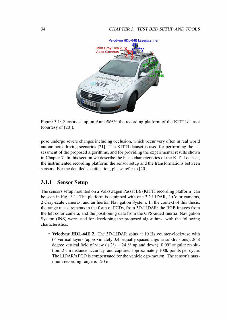
34 CHAPTER 3. TEST BED SETUP AND TOOLS
5. Experimental Evaluation
(a) Karlsruhe, Germany
xz y
yzx
Velodyne HDL-64E Laserscanner
Point Gray Flea 2Video Cameras
x yz
OXTSRT 3003GPS / IMU
x yz
OXTSRT 3003GPS / IMU
(b) Experimental Vehicle AnnieWAY (MRT/KIT)
x
yz
x
yz
x
zy
GPS/IMU(height: 0.93 m)
Velodyne laserscanner(height: 1.73 m)
Cam 0 (gray)Cam 2 (color)
Cam 1 (gray)Cam 3 (color)
2.71 m
0.81 m
0.32 m
0.27 m
0.54 m
0.06 m
All camera heights: 1.65 m
0.05 m
0.48 m
IMU-to-Velo
Velo-to-Cam
All heights wrt. road surface
Wheel axis(height: 0.30m)
1.68 m
0.80 m
1.60 m
Cam-to-CamRect& CamRect-to-Image
0.06 m
(c) Sensor Setup (Top View)
Figure 5.1.: Recording Platform. A VW Passat station wagon has been equipped with fourvideo cameras (two color and two gray scale cameras). A rotating 3D laser scanner and aGPS/IMU inertial navigation system unit have been installed for obtaining ground truth anno-tations.
stereo rig and an GPS/IMU system for localization. The trunk of our vehicle housesa PC with two six-core Intel XEON X5650 processors and a shock-absorbed RAID5 hard disk system, storing up to 4 terabytes. Our computer runs Ubuntu Linux (64bit) and a database for cognitive automobiles [80] to store the incoming data streamsin real-time.
5.2. Sensor Calibration
We took care that all sensors are carefully synchronized and calibrated [72, 150]. Toavoid drift over time, we calibrated the sensors at each day of our recordings. The
66
Figure 3.1: Sensors setup on AnnieWAY: the recording platform of the KITTI dataset(courtesy of [20]).
pose undergo severe changes including occlusion, which occur very often in real worldautonomous driving scenarios [21]. The KITTI dataset is used for performing the as-sessment of the proposed algorithms, and for providing the experimental results shownin Chapter 7. In this section we describe the basic characteristics of the KITTI dataset,the instrumented recording platform, the sensor setup and the transformations betweensensors. For the detailed specification, please refer to [20].
3.1.1 Sensor SetupThe sensors setup mounted on a Volkswagen Passat B6 (KITTI recording platform) canbe seen in Fig. 3.1. The platform is equipped with one 3D-LIDAR, 2 Color cameras,2 Gray-scale cameras, and an Inertial Navigation System. In the context of this thesis,the range measurements in the form of PCDs, from 3D-LIDAR; the RGB images fromthe left color camera, and the positioning data from the GPS-aided Inertial NavigationSystem (INS) were used for developing the proposed algorithms, with the followingcharacteristics.
• Velodyne HDL-64E 2. The 3D-LIDAR spins at 10 Hz counter-clockwise with64 vertical layers (approximately 0.4° equally spaced angular subdivisions); 26.8degree vertical field of view (+2°/− 24.8° up and down); 0.09° angular resolu-tion; 2 cm distance accuracy, and captures approximately 100k points per cycle.The LIDAR’s PCD is compensated for the vehicle ego-motion. The sensor’s max-imum recording range is 120 m.

3.1. THE KITTI VISION BENCHMARK SUITE 35
5. Experimental Evaluation
(a) Karlsruhe, Germany
xz y
yzx
Velodyne HDL-64E Laserscanner
Point Gray Flea 2Video Cameras
x yz
OXTSRT 3003GPS / IMU
x yz
OXTSRT 3003GPS / IMU
(b) Experimental Vehicle AnnieWAY (MRT/KIT)
x
yz
x
yz
x
zy
GPS/IMU(height: 0.93 m)
Velodyne laserscanner(height: 1.73 m)
Cam 0 (gray)Cam 2 (color)
Cam 1 (gray)Cam 3 (color)
2.71 m
0.81 m
0.32 m
0.27 m
0.54 m
0.06 m
All camera heights: 1.65 m
0.05 m
0.48 m
IMU-to-Velo
Velo-to-Cam
All heights wrt. road surface
Wheel axis(height: 0.30m)
1.68 m
0.80 m
1.60 m
Cam-to-CamRect& CamRect-to-Image
0.06 m
(c) Sensor Setup (Top View)
Figure 5.1.: Recording Platform. A VW Passat station wagon has been equipped with fourvideo cameras (two color and two gray scale cameras). A rotating 3D laser scanner and aGPS/IMU inertial navigation system unit have been installed for obtaining ground truth anno-tations.
stereo rig and an GPS/IMU system for localization. The trunk of our vehicle housesa PC with two six-core Intel XEON X5650 processors and a shock-absorbed RAID5 hard disk system, storing up to 4 terabytes. Our computer runs Ubuntu Linux (64bit) and a database for cognitive automobiles [80] to store the incoming data streamsin real-time.
5.2. Sensor Calibration
We took care that all sensors are carefully synchronized and calibrated [72, 150]. Toavoid drift over time, we calibrated the sensors at each day of our recordings. The
66
Figure 3.2: The top view of the multisensor configuration composed of 4 cameras, a3D-LIDAR and a GPS-aided INS (courtesy of [20]).
• Point Grey Flea 2 Camera (FL2-14S3C-C). The color camera, facing forward,has the resolution of 1.4 Mega pixels. The camera image was cropped to 1382×512pixels, and after image rectification (that is, projecting stereo images onto a com-mon image plane), the image become smaller in size (about 1242×375 pixels).The camera shutter was synchronized with the 10 Hz spinning Velodyne LIDAR.
• GPS-aided INS (OXTS RT 3003). The GPS-aided INS is a high-precision in-tegrated GPS/IMU inertial navigation system with a 100 Hz sampling rate and aresolution of 0.02 m / 0.1°. The localization data is provided with an accuracyof less than 10 cm with Real Time Kinematic (RTK) float/integer corrections en-abled. RTK is a technique that improves the accuracy of position data obtainedfrom satellite-based positioning systems.
Figure 3.2 shows the sensor configuration (top view) on the KITTI’s recording platform.The projection of a 3D-LIDAR’s PCD P into the left camera’s image plane (i.e., Cam 2(color) coordinates in Fig. 3.2) can be performed as follows:
P∗ =
Projection Matrix︷ ︸︸ ︷PC2I×R0×PL2C × P, (3.1)
where PC2I is the projection matrix from the camera coordinate system to the imageplane, R0 is the rectification matrix, and PL2C is LIDAR to camera coordinate systemprojection matrix.

36 CHAPTER 3. TEST BED SETUP AND TOOLS
3.1.2 Object Detection and Tracking DatasetsThe KITTI dataset was captured in urban areas using an ego-vehicle equipped withmultiple sensors. The data used for validation of the performance of the proposed al-gorithms is taken from ‘Object Detection Evaluation’ and ‘Object Tracking Evaluation’from KITTI Vision Benchmark Suite, as described as follows:
• Object Detection Evaluation. The KITTI Object Detection Evaluation is parti-tioned into two subsets: training and testing sets. The ‘training dataset’ contains7,481 frames of images and PCDs with 51,867 labels for nine different categories:Pedestrian, Car, Cyclist, Van, Truck, Person sitting, Tram, Misc, and Don’t care.The ‘test dataset’ consists of 7,518 frames (the class labels for the test datasetare not accessible for users). Despite having eight labeled classes (except forDon’t care labels), only Pedestrian, Car and Cyclist are evaluated in the onlinebenchmark (test dataset). It should be noted that the dataset contains objects withdifferent levels of occlusion.
• Object Tracking Evaluation. The KITTI Object Tracking Evaluation is com-posed of 21 training and 29 test sequences (of different lengths). In the KITTIdataset, objects are annotated with their tracklets, and generally, the dataset ismore focused on the evaluation of the data association problem in discriminativeapproaches.
The original KITTI Object Detection Evaluation is used for the evaluation of the pro-posed object detection algorithms in Chapter 6. During our experiments, only the ‘Car’label was considered for evaluation. To the best of our knowledge, there is no publiclyavailable dataset of sequences of images, PCDs and positioning data for evaluating sta-tionary – moving obstacle detection and multisensor generic 3D single-object trackingin driving environments (which are the main modules of the proposed obstacle detec-tion system, and are discussed in Chapter 5). Therefore, two datasets were built out ofKITTI Object Tracking Evaluation to validate the performance of the proposed obstacledetection system, as detailed in the next subsection.
3.1.3 ‘Object Tracking Evaluation’ Based Derived DatasetsIn this section we describe the ‘Object Tracking Evaluation’ based generated datasets inorder to evaluate the proposed obstacle detection system, including: stationary – movingobstacle detection and multisensor 3D single-object tracking evaluations.
• Stationary – Moving Obstacle Detection Evaluation. For the obstacle detectionevaluation task (which is composed of the ground surface estimation and station-ary – moving obstacle detection and segmentation evaluations), eight sequences

3.1. THE KITTI VISION BENCHMARK SUITE 37
Table 3.1: Detailed information about each sequence used for the stationary and movingobstacle detection evaluation.
Seq. # ofFrames
Ego-vehicleSituation
SceneCondition
ObjectType
Number of ObjectsStation. Moving
(1) 154 Moving Urban C.Y.P 11 5(2) 447 Moving Urban C.P 67 6(3) 373 Hybrid Urban C 25 14(4) 340 Moving Downtown Y.P 27 25(5) 376 Hybrid Hybrid C.Y.P 1 14(6) 209 Stationary Downtown Y.P 0 17(7) 145 Stationary Downtown P 0 10(8) 339 Moving Urban C 0 18
from the ‘Object Tracking Evaluation’ set are used. The 3D-Bounding Boxes(3D-BBs) of objects are available in the KITTI dataset. In our dataset, the 3D-BBs of stationary and moving objects were manually discriminated and labeledas being stationary or moving, by an annotator. An example of the Ground-Truth(GT) data is shown in Fig. 3.3.
The characteristics of each sequence are summarized in Table 3.1. Two of thesequences (6 and 7) were taken by a Stationary vehicle and four of them (1, 2, 4and 8) were taken by a Moving vehicle. In the remaining sequences the vehiclewent through both stationary and moving situations. The dataset is divided intotwo scene conditions: highways and roads in urban areas (Urban) or alleys andavenues in downtown areas (Downtown). Different types of objects such as Car(C), Pedestrian (P) and cYclist (Y) are available in the scenes. The total numberof objects (stationary and moving) that are visible in the perception field of thevehicle is also reported per sequence.
• 3D Single-Object Tracking Evaluation. In order to evaluate the object trackingmodule performance, eight challenging sequences out of the ‘Object TrackingEvaluation’ set were generated. In the rearranged dataset, each sequence denotesthe full trajectory of only one target object. That is, in comparison to the originaltracklets, in the composed dataset the full track of an individual object is extracted(i.e., if one scenario includes two target objects, it is considered as two sequences).The details of each sequence and the challenging factors are reported in Table3.2. Specifically, this table is divided into three main parts, as described in thefollowing.
The General Specifications This is the description of each sequence includingthe number of frames; the scene condition: Urban (U) and Downtown (D);

38 CHAPTER 3. TEST BED SETUP AND TOOLS
Figure 3.3: An example of the stationary and moving obstacle detection’s GT data.The top image shows a screenshot from the KITTI ‘Object Tracking Evaluation’ with3D-BBs being used to represent objects in the scene. The bottom figure shows thecorresponding 3D-BBs in the Euclidean space. Green and red BBs indicate moving andstationary objects, respectively. The black dots represent the bases of the 3D-BBs, andare used to evaluate the ground surface estimation.
the Ego-vehicle situation: Moving (M) and Stationary (S), and the objecttype: C, P, and Y are abbreviations for Car, Pedestrian, and cYclist, respec-tively.
The RGB Camera’s Challenging Factors It describes each sequence in termsof experiencing one of the following challenges, occlusions: No (N), Partial(P) and Full (F) occlusions; illumination variations; object pose variations,and changes in the object’s size, where Y and N are abbreviations for Yesand No, respectively.
The 3D-LIDAR’s Challenging Factors This describes the main challenges foreach of the PCD sequences, in terms of the number of object points: L and Hare abbreviations for Low and High, respectively; distance to the object: N,M, and F are abbreviations for Near, Medium, and Far, respectively, and the
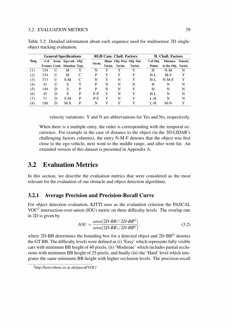
3.2. EVALUATION METRICS 39
Table 3.2: Detailed information about each sequence used for multisensor 3D single-object tracking evaluation.
Seq.General Specifications RGB Cam. Chall. Factors 3L Chall. Factors# of
FramesSceneCond.
Ego-veh.Situation
Obj.Type
Occlu.Illum.Variat.
Obj. PoseVariat.
Obj. SizeVariat.
# of Obj.Points
Distanceto the Obj.
VelocityVariat.
(1) 154 U M Y N Y Y Y H N-M N(2) 154 U M C P Y Y Y H-L M-F Y(3) 373 U S-M C N Y N Y H-L N-M-F Y(4) 41 U S Y P N N N H N N(5) 149 D S P P N N Y H N N(6) 45 D S P F-P Y N Y H-L N N(7) 71 D S-M P P-F Y N Y L-H N N(8) 188 D M-S P N Y Y Y L-H M-N Y
velocity variations: Y and N are abbreviations for Yes and No, respectively.
When there is a multiple entry, the order is corresponding with the temporal oc-currence. For example in the case of distance to the object (in the 3D-LIDAR’schallenging factors columns), the entry N-M-F denotes that the object was firstclose to the ego-vehicle, next went to the middle range, and after went far. Anextended version of this dataset is presented in Appendix A.
3.2 Evaluation MetricsIn this section, we describe the evaluation metrics that were considered as the mostrelevant for the evaluation of our obstacle and object detection algorithms.
3.2.1 Average Precision and Precision-Recall CurveFor object detection evaluation, KITTI uses as the evaluation criterion the PASCALVOC2 intersection-over-union (IOU) metric on three difficulty levels. The overlap ratein 2D is given by
IOU =area(2D-BB∩2D-BBG)
area(2D-BB∪2D-BBG), (3.2)
where 2D-BB determines the bounding box for a detected object and 2D-BBG denotesthe GT BB. The difficulty levels were defined as (i) ‘Easy’ which represents fully visiblecars with minimum BB height of 40 pixels, (ii) ‘Moderate’ which includes partial occlu-sions with minimum BB height of 25 pixels, and finally (iii) the ‘Hard’ level which inte-grates the same minimum BB height with higher occlusion levels. The precision-recall
2http://host.robots.ox.ac.uk/pascal/VOC/
40 CHAPTER 3. TEST BED SETUP AND TOOLS
curve and average precision (which corresponds to the area under the precision-recallcurve), were computed and reported over easy, moderate and hard data categories (withan overlap of 70% for ‘Car’ detection) to measure the detection performance. For moredetails, please refer to [22].
3.2.2 Metrics for Obstacle Detection EvaluationTo the extent of our knowledge, there is no standard and well-established assessmentmethodology for obstacle detection evaluation. Therefore, we defined several key per-formance metrics (mostly are defined in 3D space) to evaluate different components ofthe proposed obstacle detection system. Those metrics, which are further described inChapter 7, include the following:
• mean of Displacement Errors (mDE). Obstacle detection algorithms need someassumptions about the ground surface to discriminate between the ground and ob-stacles. For the evaluation of the ground-surface estimation process, the averagedistance from the base of the GT 3D-BBs (of labeled objects) to the estimatedground surface is computed as a measure of error (see Fig. 3.3). This is based onthe assumption that all objects lie on the true ground surface.
• The number of ‘missed’ and ‘false’ detections. As explained in the introduc-tion chapter, the term ‘obstacle’ refers to all kinds of objects. The GT labels forsuch a large and diversified group of items are not usually accessible. The ob-stacle detection evaluation is performed as follows: 1) a random subsample3 offrames (of PCDs) were selected from the dataset; 2) detections in those framesare projected into the image plane and a human observer performs a visual analy-sis in terms of missed and false obstacles, and 3) in order to consider the movingobstacles, another similar evaluation procedure is carried out for moving items.The discriminated labels (stationary and moving) in the dataset, although only asubset of all obstacles, were used to help the human observer to perform the visualanalyses.
• The position and orientation errors. To assess the accuracy of the generic 3Dobject tracking performance, the position and orientation errors were considered.The average center position errors in 2D and 3D are calculated using the Eu-clidean distance of the center of the computed 2D-BB and 3D-BB from the 2D/3DGT BBs (the GT 2D and 3D-BBs are available in the KITTI dataset). In the KITTIdataset, the GT orientation of the object is only given in terms of the Yaw anglewhich describes the object’s heading (for more details, please refer to [23]). Theorientation error in 3D is given by computing the angle between the object poseand the GT pose in x-y plane.
3Due to the great effort required to analyze the full dataset, a subsample of the dataset is used.

3.3. PACKAGES AND TOOLKITS 41
3.3 Packages and ToolkitsIn this section, we describe the You Only Look Once (YOLO) [24, 25] package. YOLOis a state-of-the-art, real-time object detection system based on Darknet4, which is anopen source Neural Network (NN) framework written in C and CUDA.
3.3.1 YOLOv2In the following, we describe YOLO and its most-recent version YOLOv2 which is usedwithin the thesis (specifically, it was used in Section 6.2).
In YOLO, object detection is defined as a regression problem and object BBs anddetection scores are directly estimated from image pixels. Taking advantage from a grid-based structure, YOLO eliminates the need for an object proposal generation step. TheYOLO network is composed by 24 convolutional layers followed by 2 Fully-Connected(FC) layers which connects to a set of BB outputs. In YOLO, the image is divided intoS× S grid regions, and the output prediction is in the form of a S× S× (B× 5+C)matrix, where B is the number of assumed BBs in each cell; C is the class probabilitieswrt to the classes, and the coefficient ‘5’ denotes 2D spatial position, width, height andthe confidence score of each BB. In YOLO [24], the input image is divided into 7× 7grid regions (i.e., S = 7), and two centers of the BBs are assumed in each grid cell(i.e., each grid predicts two BBs and one class with their associated confidence scoreswhich means a prediction of at the most 98 BBs per image). Prediction of 20 classesare considered in the YOLO (i.e., C = 20). Therefore the output will be in the shapeof a 7× 7× 30 matrix. YOLO looks at the whole image during training and test time;therefore, in addition to object appearances, its predictions are informed by contextualinformation in the image.
The most-recent version of YOLO which is used in this thesis (denoted as YOLOv2[25]) and its main differences with the original YOLO are described next. In YOLO, theconstraints of predicting only two BBs and one class limits the detection performancefor small and nearby objects. In YOLOv2 [25], the image is divided into 13× 13 gridregions, where each grid cell is responsible for predicting five object BB centers (i.e.,845 BB detections per image). In addition, instead of direct prediction of BBs fromFC layers (as in original YOLO), in YOLOv2 the FC layers are removed and BBs arecomputed by predicting corrections (or offsets) on five predefined anchor boxes. Thenetwork in YOLOv2 is composed by 19 convolutional layers and 5 max-pooling lay-ers, and (similar to YOLO) runs once on the image to predict object BBs. Some otheradditional improvements of the YOLOv2 (in comparison with YOLO) are: batch nor-malization (to speed up learning and also as a form of regularization), high resolutionclassifier and detector, and multi-scale training. For more details please refer to [25].
4http://pjreddie.com/darknet

42 CHAPTER 3. TEST BED SETUP AND TOOLS
Chapter 4
Obstacle and Object Detection: ASurvey
Contents4.1 Obstacle Detection . . . . . . . . . . . . . . . . . . . . . . . . . . . 44
4.1.1 Environment Representation . . . . . . . . . . . . . . . . . . 44
4.1.2 Grid-based Obstacle Detection . . . . . . . . . . . . . . . . . 45
4.2 Object Detection . . . . . . . . . . . . . . . . . . . . . . . . . . . . 50
4.2.1 Recent Developments in Object Detection . . . . . . . . . . . 50
4.2.2 Object Detection in ADAS Domain . . . . . . . . . . . . . . 51
The greatest challenge to any thinker isstating the problem in a way that willallow a solution.
Bertrand Russell
In this chapter, we present the state-of-the-art approaches on environment perceptionfor intelligent and autonomous vehicles focusing on the problems of obstacle and objectdetection. Specifically, obstacle detection is the problem of identifying obstacles in theenvironment. There is a related term called Detection And Tracking Moving Objects(DATMO), which is more focused on modeling dynamic generic objects (moving obsta-cles) in urban environments. Object detection is related to problems of recognizing andlocating class-specific objects in a scene.
43

44 CHAPTER 4. OBSTACLE AND OBJECT DETECTION: A SURVEY
4.1 Obstacle DetectionRobotic perception, in the context of autonomous driving, is the process by which anintelligent system translates sensory data into an efficient model of the environmentsurrounding a vehicle. Environment representation is the basis for perception tasks. Inthe following, we survey common approaches for environment representation with afocus on grid-based methods, and next, we review studies related to grid-based obstacledetection methods.
4.1.1 Environment RepresentationGiven sensory data, it needs to be processed by a perception system in order to obtaina consistent and meaningful representation of the environment surrounding the vehi-cle. Three main types of data representations are commonly used: 1) Point cloud; 2)Feature-based, and 3) Grid-based. Point cloud-based approaches directly use raw sen-sor data, with minimum preprocessing and the highest level of detail, for environmentrepresentation [26]. This approach generates an accurate representation. However, it re-quires large memory and high computational power. Feature-based methods use locallydistinguishable features (e.g., lines [27], surfaces [28], superquadrics [29]) to representthe sensor information. Feature-based approaches are concise and sparse representationmodels with no direct representation of free and unknown areas. Grid-based meth-ods discretize the space into small grid elements, called cells, where each cell containsinformation regarding the sensory space it covers. Grid-based solutions are memory-efficient, simple to implement, with no dependency to predefined features, and have theability to represent free and unknown space, which make them an efficient technique forsensor data representation in robotic applications.
Several approaches have been proposed to model sensory data using grids. Moravecand Elfes [30] presented early works on 2D grid mapping. Hebert et al. [31] proposeda 2.5D grid model (called elevation maps) that stores in each cell the estimated heightof objects above the ground level. Pfaff and Burgard [32] proposed an extended eleva-tion map to deal with vertical and overhanging objects. Triebel et al. [33] proposed aMulti-Level Surface (MLS) map that considers multiple levels for each 2D cell. Thesemethods, however, do not represent the environment in a fully volumetric (3D) way.Roth-Tabak and Jain [34] and Moravec [35] proposed a 3D occupancy grid composedof equally-sized cubic volumes (called voxels). However, it requires large amounts ofmemory since voxels are defined for the whole space, even if there are only a few mea-sured points in the environment. Specifically, LIDAR-based 3D occupancy grids canrepresent free and unknown areas by accepting a higher computation cost of ray castingalgorithms for updating the grid cells. 3D grid maps can be built faster by discardingray casting algorithms and considering only the end-points of the beams [36]. However,by ignoring ray casting algorithms, information about free and unknown spaces is lost.

4.1. OBSTACLE DETECTION 45
Table 4.1: Comparison of some of the major grid-based environment representations.L, M, F, and D are abbreviations for Level of detail, Memory, Free and unknown spacerepresentation ability, and the Dimension of representation, respectively.
Representation L M F D2D Occ. Grid [30] + + + 2Elevation Grid [31] ++ + - 2.5Extended Elev. [32] ++ + - 2.5MLS Grid [33] ++ ++ - 2.53D Occ. Grid [34] +++ +++ + 3Voxel Grid [37] +++ ++ - 3Octree [39] +++ ++ - 3
A related approach is proposed by Ryde and Hu [37], in which they store a list of occu-pied voxels over each cell of a 2D grid map. Douillard et al. [38] used a combination ofa coarse elevation map for background representation and a fine resolution voxel mapfor object representation. To reduce memory usage of fully 3D maps, Meagher [39]proposed octrees for 3D mapping. An octree is a hierarchical data structure for spa-tial subdivision in 3D. OctoMap [40] is a mature version of octree-based 3D mapping.However, the tree structure of octrees causes a more complex data access in compar-ison with a traditional 3D grid. In another attempt, Dryanovski et al. [41] proposedthe multi-volume occupancy grid, where observations are grouped into continuous ver-tical volumes (height volumes) for each map cell. Table 4.1 provides an overview ofgrid-based environment models.
4.1.2 Grid-based Obstacle Detection
Obstacle detection, which is usually built on top of grid-based representation, is one ofthe main components of perception in intelligent and autonomous vehicles [42]. In re-cent years, by increasing growth of 3D sensors such as stereo cameras and 3D-LIDARs,most of the obstacle detection techniques have been revisited to adapt themselves to 3Dsensor technologies [43]. In particular, the perception of a 3D dynamic environmentsurrounding a moving ego-vehicle requires an ego-motion estimation mechanism (inaddition to a 3D sensor). A perception system with the ability to detect stationary andmoving obstacles in dynamic 3D urban scenarios has a direct application in safety sys-tems such as collision warning, adaptive cruise control, vulnerable road users detectionand collision mitigation braking. Obstacle detection systems can be extended to includehigher level perception functionalities including Detection And Tracking Moving Ob-jects (DATMO) [44]; object detection, recognition and behavior analysis [45]. Obstacledetection algorithms need some assumptions about the ground surface to discriminatebetween the ground and obstacles [46].

46 CHAPTER 4. OBSTACLE AND OBJECT DETECTION: A SURVEY
Ground Surface Estimation
Incoming data from a 3D sensor need firstly to be processed for ground surface esti-mation and subsequently for obstacle detection. Ground surface and obstacle detectionhave a strong degree of dependency because the obstacles (e.g., trees, walls, poles, fire-plugs, vehicles, pedestrians, and cyclists) are all located on the surface that representsthe roadway and the roadside. Many of the methods assume that the ground is flat andeverything that stands up from the ground is considered as obstacles [47], [48], [49].However, this simple assumption is overridden in most of the practical scenarios. In[28] the ground surface is detected by fitting a plane using RANSAC on the point cloudfrom the current time instance. This method only works well when the ground is planar.Non-planar grounds, such as undulated roads, curved uphill and downhill ground sur-faces, sloped terrains or situations with big rolling and pitch angles of the roads remainunsolved. The ‘V-disparity’ approach [50] is widely used to detect the road surface fromthe disparity map of stereo cameras. However, disparity is not a natural way to represent3D Euclidean data and it can be sensitive to roll angle changes. A comparison between‘V-disparity’ and Euclidean space approaches is given in [51]. In [52] a combination ofRANSAC [53], region growing and Least Square (LS) fitting is used for the computationof the quadratic road surface. Though it is effective, yet it is limited to the specific casesof planar or quadratic surfaces. Petrovskaya [54] proposed an approach that determinesground readings by comparing angles between consecutive readings from Velodyne LI-DAR scans. Assuming A, B, and C are three consecutive readings, the slope betweenAB and BC should be near zero if all three points lie on the ground. A similar methodwas independently developed in [55]. In [56] the ground points are detected by com-paring adjacent beams, as the difference between adjacent beams is lower at objectsand higher at the ground. Mertz et al. [57] build an Elevation grid by subtracting thestandard deviation from the average height of the points within each cell. The cellswith Elevation value lower than a certain threshold are considered as the ground cells.In [58], all objects of interest are assumed to reside on a common ground plane. Thebounding boxes of objects, from the object detection module, are combined with stereodepth measurements for the estimation of the ground plane model.
Generic Object Tracking
Generic (or model-free) object tracking is an essential component in the obstacle de-tection pipeline. Using tracking, an ego-vehicle can predict its surrounding objects’locations and behaviors, and based on that make proper decisions and plan next actions.This section gives a brief overview of object tracking algorithms using multimodal per-ception systems of autonomous vehicles. Object tracking algorithms can be divided intotracking by detection and model-free categories as detailed in the sequel.
• Tracking by Detection. Discriminative object trackers localize the object us-

4.1. OBSTACLE DETECTION 47
observer
obstacle
(a) (b) (c) (e) (f)(d)
Figure 4.1: Some approaches for the appearance modeling of a target object. (a) repre-sents a scan of a vehicle which is split up by an occlusion from top view [59] , (b) thecentroid (point model) representation, (c) 2D rectangular [60] or 2.5D box [56] shapebased representations, (d) 2.5D grid, 3D voxel grid [48, 61] or octree data structure-based representation [49, 62], (e) object delimiter-based representation [63], and (f) 3Dreconstruction of the shape of the target object [64, 65].
ing a pre-trained (supervised) detector (e.g., DPM [66]) that learns a decisionboundary between the appearance of the target object and other objects and ob-stacles, and next link-up the detected positions over time. Many approaches[67, 68, 69, 70, 71, 72] have been proposed for discriminative object trackingbased on monocular cameras, with most of them focused on the data associationproblem. An overview of such approaches is given in the ‘KITTI Object TrackingEvaluation Benchmark’1, MOT15 [73] and MOT16 [74]. However, the require-ment of having all object categories being previously known and trained limits theapplication of discriminative approaches.
• Model-Free. To have a reliable perception system for autonomous cars in real-world driving scenarios a generic object tracker [63, 75, 76, 77] is also required. Ageneric tracker should be able to track all kinds of objects, even if their existence isnot previously predicted or trained. It is generally assumed that the initial positionof the object is given (e.g., using a motion detection mechanism). Generativemethods build a model to describe the appearance of the object (in the initialframe) and then look for its next occurrence by searching for the region mostsimilar to the model. To handle the appearance variations of the target object,the object model is often updated online. The simplest representation of a targetobject considers the centroid of object points, so-called the point model. The pointmodel is feasible even with a few number of object points. However, a richerappearance modeling can be exploited to capture objects physical properties (seeFig. 4.1). Generic object tracking, integrated in the obstacle detection system, isfurther discussed in the following.
1http://www.cvlibs.net/datasets/kitti/eval tracking.php
48 CHAPTER 4. OBSTACLE AND OBJECT DETECTION: A SURVEY
Obstacle Detection and DATMO
This section briefly reviews grid-based obstacle detection in dynamic environments.Some approaches [48, 60, 61] detect and track generic dynamic objects based on theirmotion. This group of methods is the most widely used and is closely related to theDetection and Tracking of Moving Objects (DATMO) approaches [44]. The BayesianOccupancy Filter (BOF) is a well known grid-based DATMO. In BOF, Bayesian filteringis adapted to the occupancy grids to infer the dynamic grids, followed by segmentationand tracking (using Fast Clustering and Tracking Algorithm (FCTA) [78]), to providean object level representation of the scene [79]. Motion detection can be achieved bydetecting changes that occur between two or three consecutive observations (which canbe interpreted as ‘frame differencing’) [60].
Detection of motion can also be achieved by building a consistent static model ofthe scene, called the background model, and then finding deviations from the model ineach incoming frame [49]. This process can be referenced as ‘background modelingand subtraction’. The background model is usually a short-term map of the surroundingenvironment of the ego-vehicle. Generally, the static background model is built by com-bining the ego-vehicle localization data and a representation of 3D sensor inputs such as:PCD [60], 2.5D Elevation grid [63], Stixel (sets of thin and vertically oriented rectan-gles) [47, 80], voxel grid [48, 61] or octree data structure-based representation [49, 62].Ego-motion estimation is usually achieved using Visual Odometry [48], INS [63], vari-ants of ICP scan matching algorithm [61] or a combination of them [49]. In Broggi et al.[48] approach, voxels are used to represent 3D space, and the ego-motion is estimatedusing Visual Odometry. A color-space segmentation is performed on the voxels, andthe voxels with similar features are grouped to form obstacles. The ego-motion is usedto distinguish between stationary and moving obstacles. Finally, the geometric centerof each obstacle is computed, and a KF is applied to estimate its velocity and position.Azim and Aycard [49] proposed an approach based on the inconsistencies between ob-servation and local grid maps represented by an Octomap (which is a 3D occupancygrid with an octree structure) [40]. Obstacles are segmented using DBSCAN, followedby a KF and Global Nearest Neighborhood (GNN) data association for tracking. Next,an adaboost classifier is used for object classification. Moosmann and Stiller [65] useda local convexity based segmentation method for object hypotheses detection. A com-bination of KF and ICP is used for tracking generic moving objects and a classificationmethod for managing tracks. Their method includes the 3D reconstruction of the shapeof the moving objects. Hosseinyalamdary et al. [59] used prior Geospatial InformationSystem (GIS) map to reject outliers. They tracked moving objects in a scene using KF,with Constant Velocity process model (CV-KF) and used ICP for pose estimation. De-wan et al. [81] detect motions between consecutive scans using RANSAC and use aBayesian approach to segment and track multiple objects in 3D-LIDAR data.
The majority of these approaches have only been developed for the detection and

4.1. OBSTACLE DETECTION 49
Table 4.2: Some of the recent obstacle detection and tracking methods for autonomousdriving applications. Cam., SV, mL, 2L, and 3L are abbreviations for Camera, StereoVision, multilayer LIDAR, 2D-LIDAR, and 3D-LIDAR, respectively. Col., Vel., Mot.,and Spat. are abbreviations for Color, Velocity, Motion, and Spatial, respectively.
Ref. 3D Sens. Ego-motionEstimation
Motion Det. &Segmentation
ObjectRepresent.
Obj. SearchMechanism
Obj. ModelUpdate
[79] SV, 2L Odometry FCTA 2D Occ. Vel. Bayesian –[63] SV GNSS, INS Obj. Delimit. DEM PF KF[61] mL ICP Motion Voxel EKF –[59] 3L, GIS INS – PCD CV-KF –[75] SV V-Odometry Multi Scale Voxel KF, MHT Weighted ICP[65] 3L – Local Convexity PCD CV-KF ICP, Accum.[47] SV V-Odometry Mot. Spat. Shape Stixel 6D-KF –[64] 3L, Cam. INS – Col. PCD CV-KF ICP, Accum.[81] 3L DGPS/IMU Motion PCD Bayesian –[48] SV V-Odometry Color Space Voxel KF –[49] 3L INS, ICP DBSCAN Octree KF, GNN –[60] 3L INS Motion 2D Rect. PF CV-KF
tracking of generic moving objects. However, in real-world applications, static obstaclesshould also be taken into account. Segmentation-based approaches are proposed topartition the PCD into perceptually meaningful regions that can be used for obstacledetection. Osep et al. [75] used the PCD generated from a disparity map (obtainedfrom a stereo camera pair) to find and track generic objects. They suggested a two-stagesegmentation approach for multiscale object proposal generation, followed by MultiHypothesis Tracking (MHT) at the level of the object proposals. Vatavu et al. [63] builta Digital Elevation Map (DEM) from PCD obtained from a stereo vision system. Theysegmented obstacles by extracting free-form object delimiters. The object delimiters arerepresented by their positions and geometries, and then tracked using Particle Filters(PFs). KFs are used for adapting object delimiter models. Pfeiffer and Franke [47]used a stereo vision system for acquiring 3D PCD and Visual Odometry for ego-motionestimation. They used Stixels for the environment representation. Dynamic stixels aresegmented based on the motion, spatial and shape constraints, and are tracked by aso-called 6D-vision KF [82], which is a framework for the simultaneous estimation of3D-position and 3D-motion. In another approach, focused on the problem of genericobject tracking, Held et al. [64] combined a PCD with a 2D camera image to constructan up-sampled colored PCD. They used a color-augmented search algorithm to align thecolored PCDs from successive time frames. Assuming a known initial position of theobject, they utilized 3D shape, color data and motion cues in a probabilistic frameworkto perform joint 3D reconstruction and tracking. They showed that the accumulateddense model of the object leads to a better object velocity estimate. A summary of themost representative obstacle detection and tracking approaches is provided in Table 4.2.

50 CHAPTER 4. OBSTACLE AND OBJECT DETECTION: A SURVEY
4.2 Object DetectionThis section gives an overview of object detection, the related fusion methods and recentadvancements applied in ADAS and ITS domains.
4.2.1 Recent Developments in Object DetectionThe state-of-the-art in object detection is primarily concentrated on processing colorimages. Object detection can be divided into pre and post-Deep learning arrival.
Non-ConvNet Approaches
Before the recent advancement of Deep Learning (specifically ConvNets) that revolu-tionized object classification and consecutively the object detection field, the literaturewere mainly focused on using hand crafted features and traditional classification tech-niques (e.g., SVM, AdaBoost, Random Forest). Some of the major contributions in theobject detection field, before the Deep Learning era, are listed below:
• Cascade of weak classifiers. Viola and Jones [83] proposed one of the earlyworks for object detection. They used Haar features and performed object de-tection by applying Adaboost training and cascade classifiers based on sliding-window principle.
• Histogram of Oriented Gradients (HOG). Dalal and Triggs [84] introduced ef-ficient HOG features based on edge directions in the image. They performed lin-ear SVM classification on sub-windows extracted from the image using a sliding-window mechanism.
• Deformable Parts Model (DPM). Proposed by Felzenszwalb et al. [85], DPM isa graphical model that is designed to cope with object deformations in the image.DPM assumes that an object is constructed by its parts. It uses HOG and linearSVM, again on a sliding window mechanism.
• Selective Search (SS). Uijlings et al. [86] proposed SS to generate a set of data-driven, class-independent object proposals and avoid using conventional sliding-window exhaustive search. SS works based on hierarchical segmentation usinga diverse set of cues. They used SS to create a Bag-of-Words based localizationand recognition system.
ConvNet based Approaches
The remarkable success of ConvNets as an optimal feature extractor for image classi-fication/recognition made a huge impact on the object detection field as demonstrated

4.2. OBJECT DETECTION 51
by LeCun et al. [87] and, more recently, by Krizhevsky et al. [88]. Currently, the bestperforming object detectors use ConvNets and are summarized below.
• Sliding-window ConvNet. Following the traditional object detection paradigm,ConvNets were initially employed using the sliding-window mechanism (but in amore efficient way), like in the Overfeat framework as proposed by Sermanet etal. [89].
• Region-based ConvNets. In R-CNN [90], SS [86] is used for object proposalgeneration, pre-trained ConvNet on ImageNet (fine-tuned by PASCAL VOC dataset)for feature extraction, and linear SVM for object classification and detection. In-stead of doing ConvNet-based classification for thousands of SS-based generatedobject proposals, which is slow, Fast R-CNN [91] uses Spatial Pyramid Poolingnetworks (SPPnets) [92] to pass the image through the convolutional layer once,followed by an end-to-end training. In Faster R-CNN [93, 94] a Region ProposalNetwork (RPN), a type of Fully-Convolutional Network (FCN) [95], is introducedfor region proposal generation. It increases the run-time efficiency and accuracyof the object detection system.
• Single Shot Object Detectors. YOLO (You Only Look Once) [24, 25] and SSD(Single Shot Detector) [96] model object detection as a regression problem and tryto eliminate the object proposal generation step. These approaches are based on asingle ConvNet followed by a non-maximum suppression step. In these methods,the input image is divided into a grid (7× 7 grid for YOLO and 9× 9 for SSD)where each grid cell is responsible for predicting a pre-determined number ofobject BBs. In the SSD approach, hard negative mining is performed, and sampleswith highest confidence loss are selected. Two main disadvantages of this class ofmethods are i) they impose hard constraints on the bounding box prediction (e.g.,in YOLO each grid cell can predict only two BBs) and ii) the detection of smallobjects can be very challenging. The SSD approach tried to solve the secondproblem with the help of additional data augmentation for smaller objects.
4.2.2 Object Detection in ADAS Domain
Object detection is a crucial component of sensor-based perception systems for ad-vanced driver assistance systems (ADAS) and for autonomous driving. This sectiongives an overview of object detection and the related fusion methods in IV and ITSdomains.

52 CHAPTER 4. OBSTACLE AND OBJECT DETECTION: A SURVEY
Vision-based Object Detection
Despite remarkable advancements in object detection, designing an object detectionsystem for real-world driving applications is still a very challenging problem.
Yebes et al. [97] modified DPM [85] to incorporate 3D-aware HOG-based featuresextracted from color images and disparity maps. Disparity maps are computed fromeach pair of left-right images of stereo cameras employing the Semi-Global Matching(SGM) [98] method. The DPM object detector is trained on 3D-aware features. Xianget al. [99] introduced a ConvNet-based region proposal network that uses subcategoryinformation to guide the proposal generating process. In their approach Fast R-CNN[91] is modified by injecting subcategory information (using 3D Voxel Patterns [100] assubcategories) into the network for joint detection and subcategory classification. Caiet al. [101] proposed a multi-scale object detection based on the concept of rescal-ing the image multiple times so that the classifier can match all possible object sizes.Their approach consists of two ConvNet-based sub-networks: a proposal sub-networkand a detection sub-network learned end-to-end. Chabot et al. [102] introduced DeepMANTA, a framework for 2D and 3D vehicle detection in monocular images. In theirmethod, inspired by the Region Proposal Network (RPN) [93], vehicle proposals arecomputed and then refined to detect vehicles. They optimized ConvNet for six tasks:region proposal, detection, 2D box regression, part localization, part visibility and 3Dtemplate prediction. Chen et al. [103] generate 3D proposals by assuming a prior onthe ground plane (using calibration data). Proposals are initially scored based on somecontextual and segmentation features, followed by rescoring using a version of Fast R-CNN [91] for 3D object detection. Yang et al. [104] approach is based on the rejectionof negative object proposals using convolutional features and cascaded classifiers.
3D-LIDAR-based Object Detection
Recently, 3D-LIDARs started to become used for high-level perception tasks like objectdetection. This subsection gives a concise overview of vehicle detection approachesusing 3D-LIDARs.
Behley et al. [105] propose a segmentation-based object detection using LIDARrange data. A hierarchical segmentation is used to reduce the over- and under-segmentationeffects. A mixture of multiple bag-of-word (mBoW) classifiers is applied to classify ex-tracted segments. Finally, a non-maximum suppression is used considering the hierar-chy of segments. In the Wang and Posner [106] approach, LIDAR points together withtheir reflectance values are discretized into a coarse 3D voxel grid. A 3D sliding windowdetection approach is used to generate the feature grid. At each window location, thefeature vectors contained within its bounds are stacked up into a single long vector andpassed to a classifier. A linear SVM classifier scores each window location and returnsa detection score. Li et al. [107] used a 2D Fully-Convolutional Network (FCN) in a

4.2. OBJECT DETECTION 53
Table 4.3: Related work on 3D-LIDAR-based object detection.
Ref. Modality Representation Detection Technique[105] Range PCD Hierarchical Seg. + BoW[108] Range PCD 3D-FCN[107] Range Top view 2D-FCN[106] Range + Reflectance Voxel Sliding-window + SVM[109] Range + Reflectance Voxel Feat. Learning + Conv. Layers + RPN[110] Color + Range Front view Sliding-window + DPM/SVM[111] Color + Range Front view Sliding-window + RF[112] Color + Range Front view Seg.-based Proposals + ConvNet[113] Color + Range + Reflectance Front + Top views Top view 3D Proposals + ConvNet
2D point map (top-view projection of 3D-LIDAR range data) and trained it end-to-endto build a vehicle detection system based only on 3D-LIDAR range data. Li [108] ex-tended it to a 3D Fully-Convolutional Network (FCN) to detect and localize objects as3D boxes from LIDAR point cloud data. In a similar approach, Zhou and Tuzel [109]proposed a method that generates 3D detection directly from the PCD. Their methoddivides the space into voxels, decodes points within the voxel into a feature vector, andthen a RPN is applied to provide 3D detections.
3D-LIDAR and Camera Fusion
Although there is a rich literature on multisensor data fusion as recently surveyed byDurrant-Whyte and Henderson [114], only a small number of works addresses multi-modal and multisensor data fusion in object detection. Fusion-based object detectionapproaches can be divided based on the abstraction level where the fusion takes place,namely i) low-level (early) fusion: combines sensor data to create a new set of data; ii)mid-level fusion: integrates features, and iii) high-level (late or decision-level) fusion:combines the classified outputs; and iv) multi-level fusion: integrates different levelsof data abstraction (also see Section 2.1.3). This subsection surveys the state-of-the-art fusion techniques using vision and 3D-LIDAR in the multimodal object detectioncontext.
Premebida et al. [110] combine Velodyne LIDAR and color data for pedestrian de-tection. A dense depth map is computed by up-sampling LIDAR points. Two DPMsare trained on depth maps and color images. The DPM detections on depth maps andcolor images are fused to achieve the best performance using a late re-scoring strategy(by applying SVM on features like BB’s sizes, position, scores and so forth). Gonzalezet al. [111] use color images and 3D-LIDAR-based depth maps as inputs, and extractHOG and Local Binary Patterns (LBP) features. They split training set samples in dif-ferent views to take into account different poses of objects (frontal, lateral, etc.) andtrain a separate random forest of local experts for each view. They investigated feature-

54 CHAPTER 4. OBSTACLE AND OBJECT DETECTION: A SURVEY
Table 4.4: Some recent related work on 3D-LIDAR and camera fusion. In the table, ifmore than one fusion strategy is experimented in a method, the best-performing solutionfor that method is emphasized with a larger red check mark.
Reference Early Mid Late Multi TechniquePremebida et al. [110] SVM Re-scoringGonzalez et al. [111] Ensemble VotingSchlosser et al. [115] ConvNetChen et al. [113] ConvNetOh and Kang [112] ConvNet/SVM
level and late fusion approaches. They combine color and depth modalities at featurelevel by concatenating HOG and LBP descriptors. They train individual detectors oneach modality and use an ensemble of detectors for the late fusion of different viewsdetection. They achieved a better performance with the feature-level fusion scheme.Schlosser et al. [115] explore the ConvNet-based fusion of 3D-LIDAR and color im-age at different levels of representation for pedestrian detection. They compute HHA(horizontal disparity, height, angle) data channels [116] from LIDAR data. They showthat the late-fusion of HHA features and color images achieve better results. Chen etal. [113] proposed a multi-view object detection using deep learning. They used 3D-LIDAR top and front views and color image data as inputs. The top view LIDAR data isused to generate 3D object proposals. The 3D proposals are projected into three viewsfor obtaining region-wise features. A region-based feature fusion scheme is used for theclassification and orientation estimation. This approach enables interactions of differentintermediate layers from different views. Oh and Kang [112] use segmentation-basedmethods for object proposal generation from LIDAR’s point cloud data and a color im-age. They use two independent ConvNet-based classifiers to classify object candidatesin color image and LIDAR-based depth map and combine the classification outputs atdecision level using convolutional feature maps, category probabilities, and SVMs. Ta-ble 4.3 provides a review of object detection approaches that incorporate 3D-LIDARdata, in terms of detection techniques. Table 4.4 provides an overview of the architec-ture of fusion approaches that use 3D-LIDAR and camera data.
In this chapter, the state-of-the-art approaches to the problems of obstacle and objectdetection was surveyed. The objective of this dissertation is to push forward the state-of-the-art in multisensor multimodal obstacle and object detection domain which are thecore modules of perception system for autonomous driving.

Part II
METHODS AND RESULTS
55


Chapter 5
Obstacle Detection
Contents5.1 Static and Moving Obstacle Detection . . . . . . . . . . . . . . . . 58
5.1.1 Static and Moving Obstacle Detection Overview . . . . . . . 58
5.1.2 Piecewise Ground Surface Estimation . . . . . . . . . . . . . 58
5.1.3 Stationary – Moving Obstacle Detection . . . . . . . . . . . . 64
5.2 Extension of Motion Grids to DATMO . . . . . . . . . . . . . . . . 69
5.2.1 2.5D Grid-based DATMO Overview . . . . . . . . . . . . . . 69
5.2.2 From Motion Grids to DATMO . . . . . . . . . . . . . . . . 69
5.3 Fusion at Tracking-Level . . . . . . . . . . . . . . . . . . . . . . . 74
5.3.1 Fusion Tracking Overview . . . . . . . . . . . . . . . . . . . 74
5.3.2 3D Object Localization in PCD . . . . . . . . . . . . . . . . 75
5.3.3 2D Object Localization in Image . . . . . . . . . . . . . . . 78
5.3.4 KF-based 2D/3D Fusion and Tracking . . . . . . . . . . . . . 80
In this chapter, we present the proposed obstacle detection approach to continuouslyestimate the ground surface and segment stationary and moving obstacles, followed byan extension of the proposed obstacle segmentation approach to DATMO, and the fusionof 3D-LIDAR’s PCD with color camera data for the object tracking function of DATMO.
Parts of this chapter have been published in one journal article and 4 book chapter,conference, and workshop proceedings: Journal of Robotics and Autonomous System[117], the Second Iberian Robotics Conference [118], IEEE Intelligent TransportationSystems Conferences [119, 120], and the Workshop on Planning, Perception and Navi-gation for Intelligent Vehicles [121].
57

58 CHAPTER 5. OBSTACLE DETECTION
5.1 Static and Moving Obstacle DetectionIn this section, considering data from a 3D-LIDAR and a GPS-aided INS mounted on-board an instrumented vehicle, a 4D approach (utilizing both 3D spatial and time data)is proposed for ground surface modeling and obstacle detection in dynamic urban envi-ronments. The system is composed of two main modules: 1) a ground surface estima-tion based on piecewise plane fitting, and 2) a voxel grid model for static and movingobstacle detection and segmentation.
5.1.1 Static and Moving Obstacle Detection OverviewFig. 5.1 presents the architecture of the proposed method. The proposed method com-prises two phases: 1) ground surface estimation: a temporal sequence of 3D-LIDARdata and GPS-aided INS positioning data are integrated to form a dense model of thescene. A piecewise surface estimation algorithm, based on a ‘multi-region’ strategyand Velodyne LIDAR scans behavior, is applied to fit a finite set of multiple planesusing RANSAC method (that fits the road and its vicinity), and 2) static and movingobstacles segmentation: the estimated ground model is used to separate the groundfrom non-ground 3D-LIDAR points (which represent obstacles that are standing on theground). The voxel representation is employed to quantize 3D-LIDAR data for efficientfurther-processing. The proposed approach detects moving obstacles using discrimi-native analysis and ego-motion information, by integrating and processing informationfrom previous measurements.
5.1.2 Piecewise Ground Surface EstimationThis section starts by presenting the process of dense PCD generation, which will beused for the ground surface estimation.
Dense Point Cloud Generation
The dense PCD construction begins by transforming the PCDs from the ego-vehicle co-ordinates to the world coordinate system using INS positioning data. This transforma-tion is further refined by PCD down-sampling using Box Grid Filter (BGF)1, followedby PCDs alignment using ICP algorithm [122]. This process, detailed in the following,is summarized in Algorithm 2.
Let Pi denote a 3D PCD in the current time i, and P = Pi−m, · · · ,Pi−1,Pi is aset composed of the current and m previous PCDs. Using a similar notation, let T =Ti−m, · · · ,Ti−1,Ti be the set of vehicle pose parameters, a 6 DOF pose in Euclidean
1The MATLAB pcdownsample function is used in our implementation.

5.1. STATIC AND MOVING OBSTACLE DETECTION 59
Piecewise Ground Surface Estimation
Static - Moving Obstacle Detection
Dense PCD
Generation
Piecewise Plane
Fitting
Integrated PCDs
A Set of
PCDs
INS Data
Ground
Parameters
Ground – Obstacle
Segmentation
Static - Moving
Obstacle Detection
Voxel Grids
A Set of
PCDs
INS Data
Static and
Moving Voxels Ground
Param.
G
DT
P
GT
P
, DP
Figure 5.1: Architecture of the proposed obstacle detection system.
Algorithm 2 Dense Point Cloud Generation.1: Inputs: PCDs: P and Ego-vehicle Poses: T2: Output: Dense PCD: D3: for scan k = i−m to i do4: Tk← ICP (BGF (GI (Pi,Ti)), BGF (GI (Pk,Tk))) . updated transformation5: D←Merge (Pk,Ti, Tk)6: end for
space, given by a high precision GPS-aided INS positioning system. The transformationTk = (Rk | tk) consists of a 3×3 rotation matrix Rk and a 3×1 translation vector tk, whenk ranges from i−m to i. The function GI (Pk,Tk) denotes the transformation of a PCD Pkfrom ego-vehicle to the world coordinate system using: Rk×Pk + tk. A Box Grid Filteris used for down-sampling the PCDs. BGF partitions the space into voxels and averages(x,y,z) value of points within each voxel. This step makes the PCD registration faster,while keeping the result accurate. ICP is applied for minimizing the difference betweenevery PCD and the considered reference PCD. The down-sampled version of the currentPCD Pi is used as the reference ‘the fixed PCD’, and then the 3D rigid transformation foraligning other down-sampled PCDs Pk ‘moving PCDs’ with the fixed PCD is estimated.Assuming Tk as the updated GPS-aided INS transformation (i.e., after applying ICP),the so called dense PCD Di is obtained using the ‘Merge’ function, by transforming thePCDs P into the current coordinates’ system of the ego-vehicle using the parameters ofTk = (Rk | tk) and Ti = (Ri | ti) by
Di =⋃i
k=i−m R−1i × ((Rk×Pk + tk)− ti), (5.1)

60 CHAPTER 5. OBSTACLE DETECTION
Figure 5.2: The generated dense PCD of a traffic pole before and after applying BoxGrid Filter and ICP algorithm. The red rectangle in the top image shows the traffic pole.Bottom left shows the generated dense PCD only using GPS-aided INS localizationdata. Bottom right shows the result obtained after applying BGF and ICP steps to furtheralign consecutive PCDs and to reduce the localization error. The sparse points on rightside of the pole (bottom right image) correspond to chain that exists between poles.Different colors encode distinct LIDAR scans. The dense PCDs were rotated regardingtheir original position in the image above to better evidence the difference.
where ∪ defines the union operation. The integrated PCD D is cropped to the localgrid: D←Crop(D). Note that the subscript i has been omitted to simplify notation. Anexample of a dense PCD generated using Tk transformation is shown in Fig. 5.2.
Piecewise Plane Fitting
A piecewise plane fitting algorithm is then applied to D in order to estimate the groundgeometry. Existing methods in the literature are mainly developed to estimate specifictypes of ground surface (e.g., planar or quadratic surfaces). In comparison to the pre-vious methods, we contribute with a piecewise plane fitting that is able to estimate anarbitrary ground surface (e.g., a ground with a curve profile). The proposed algorithm iscomposed by four steps: 1) Slicing, 2) Gating, 3) Plane Fitting, and 4) Validation. First,a finite set of regions on the ground are generated in accordance to the car orientation.

5.1. STATIC AND MOVING OBSTACLE DETECTION 61
0
h
N0 1
2
3
0
1k k
kS
x
y
z
V
N
0
Figure 5.3: Illustration of the variable-size ground slicing for η = 2. Velodyne LIDARscans are shown as dashed green lines.
These regions (hereafter called ‘slices’) are variable in size and follow the geometricalmodel that governs the Velodyne LIDAR scans. Second, a gating strategy is applied tothe points in each slice using an interquartile range method to reject outliers. Then, aRANSAC algorithm is used to robustly fit a plane to the inlier set of 3D data points ineach slice. At last, every plane parameter is checked for acceptance based on a valida-tion process that starts from the closest plane to the farthest plane.
• Slicing. This process starts from the initial region, defined by the slice S0, cen-tered in the vehicle coordinates V with the radius of λ0 = 5 m, as illustrated inFig. 5.3. This is the closest region to the host vehicle, with the densest number ofpoints and with less localization errors. It is reasonable to assume that the planefitted to the points belonging to this region is estimated with more confidenceand provides the best fit among all the remaining slices, hence this plane can beconsidered as the ‘reference plane’ for the validation task.
The remaining regions (in the area between λ0 and λN), having increasing sizes,are obtained by a strategy that takes into account the LIDAR-scans behavior: as-sumed to follow a tangent function law. Each slice (or region) begins from theendmost edge of the previous slice in the vehicle movement direction. Accord-ing to the model illustrated in Fig. 5.3, the edge of the slice Sk is given by thefollowing tangent function:
λk = h · tan(α0 + k ·η ·∆α), k : 1, ...,N (5.2)
where α0 = arctan(λ0/h) and h is the elevation of the Velodyne LIDAR to theground (h ≈ 1.73 m, provided in the dataset, see Fig. 3.2); N is the total numberof slices given by N = b(αN −α0)/(η ·∆α)c; ∆α is the angle between scans inelevation direction (∆α ≈ 0.4°), and b.c denotes truncation operation (the floorfunction). Here, η is a constant that determines the number of ∆α intervals usedto compute slice sizes (it is related to the number of LIDAR readings in eachslice). For η = 2, as represented in Fig. 5.3, at least two ground readings of a
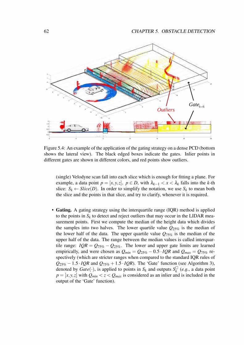
62 CHAPTER 5. OBSTACLE DETECTION
6kGate
(a)
(b)
Outliers
Figure 5.4: An example of the application of the gating strategy on a dense PCD (bottomshows the lateral view). The black edged boxes indicate the gates. Inlier points indifferent gates are shown in different colors, and red points show outliers.
(single) Velodyne scan fall into each slice which is enough for fitting a plane. Forexample, a data point p = [x,y,z], p ∈ D, with λk−1 < x < λk falls into the k-thslice: Sk ← Slice(D). In order to simplify the notation, we use Sk to mean boththe slice and the points in that slice, and try to clarify, whenever it is required.
• Gating. A gating strategy using the interquartile range (IQR) method is appliedto the points in Sk to detect and reject outliers that may occur in the LIDAR mea-surement points. First we compute the median of the height data which dividesthe samples into two halves. The lower quartile value Q25% is the median ofthe lower half of the data. The upper quartile value Q75% is the median of theupper half of the data. The range between the median values is called interquar-tile range: IQR = Q75%−Q25%. The lower and upper gate limits are learnedempirically, and were chosen as Qmin = Q25%− 0.5 · IQR and Qmax = Q75% re-spectively (which are stricter ranges when compared to the standard IQR rules ofQ25%− 1.5 · IQR and Q75% + 1.5 · IQR). The ‘Gate’ function (see Algorithm 3),denoted by Gate(·), is applied to points in Sk and outputs Sk (e.g., a data pointp = [x,y,z] with Qmin < z < Qmax is considered as an inlier and is included in theoutput of the ‘Gate’ function).

5.1. STATIC AND MOVING OBSTACLE DETECTION 63
mindmax
1kQ
1k
min1kQ
k1k
kGate
1KZ
1K 1kGate
kS
Figure 5.5: The piecewise RANSAC plane fitting process. Dashed orange shows thelower and upper gate limits. Dashed black rectangles show the gate computed for theoutlier rejection task. Solid green lines show the estimated plane using RANSAC ina lateral view. Dashed green line shows the continuation of the Sk’s fitted plane inslice Sk+1. The distance (δZk+1) and angle (δψk+1) between two consecutive planesare shown in red. Dashed magenta lines show the threshold that is used for the groundobstacle segmentation task. Points under dashed magenta lines are considered as groundpoints. The original PCD is represented using filled gray circles.
• RANSAC Plane Fitting. The RANSAC method [53] robustly fits a mathemati-cal model to a dataset containing outliers. Differently from the Least Square (LS)method that directly fits a model to the whole dataset (when outliers occur LSwill not be accurate), RANSAC estimates parameters of a model using differentobservations from data subsets. In order to perform this stage efficiently, a sub-sample of the filtered PCD in Sk is selected and a plane is fitted to it using the3-point RANSAC algorithm. In each iteration, the RANSAC approach randomlyselects three points from the dataset. A plane model is fitted to the three pointsand a score is computed as the number of inliers points whose distance to theplane model is below a given threshold. The plane having the highest score ischosen as the best fit to the considered data. A given plane, fitted to the roadand its vicinity pavement, is denoted as akx+ bky+ ckz+ dk = 0, and stored byGk← [ak,bk,ck,dk].
• Validation of Piecewise Planes. Due to the broader area and denser points (withless errors in LIDAR measurements) in the immediate slice S0, the plane com-puted from this region’s points has the best fit among the other slices, and henceis considered as the ‘reference plane’ G0. According to the tangent based slicing(5.2) the number of LIDAR’s ground readings in the other slices should be almostequal (see Fig. 5.3). The validation process starts from the closest plane G1 to
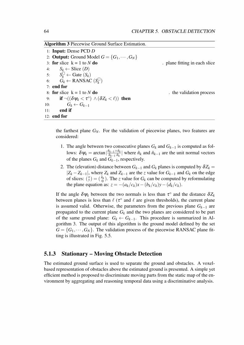
64 CHAPTER 5. OBSTACLE DETECTION
Algorithm 3 Piecewise Ground Surface Estimation.1: Input: Dense PCD D2: Output: Ground Model G = G1, · · · ,GN3: for slice k = 1 to N do . plane fitting in each slice4: Sk← Slice (D)5: Sk ← Gate (Sk)6: Gk← RANSAC (Sk )7: end for8: for slice k = 1 to N do . the validation process9: if ¬((δψk < τ°) ∧ (δZk < `)) then
10: Gk← Gk−111: end if12: end for
the farthest plane GN . For the validation of piecewise planes, two features areconsidered:
1. The angle between two consecutive planes Gk and Gk−1 is computed as fol-lows: δψk = arctan | nk−1×nk
nk−1·nk| where nk and nk−1 are the unit normal vectors
of the planes Gk and Gk−1, respectively.
2. The (elevation) distance between Gk−1 and Gk planes is computed by δZk =|Zk−Zk−1|, where Zk and Zk−1 are the z value for Gk−1 and Gk on the edgeof slices: ( x
y) = (λk0 ). The z value for Gk can be computed by reformulating
the plane equation as: z =−(ak/ck)x− (bk/ck)y− (dk/ck).
If the angle δψk between the two normals is less than τ° and the distance δZkbetween planes is less than ` (τ° and ` are given thresholds), the current planeis assumed valid. Otherwise, the parameters from the previous plane Gk−1 arepropagated to the current plane Gk and the two planes are considered to be partof the same ground plane: Gk ← Gk−1. This procedure is summarized in Al-gorithm 3. The output of this algorithm is the ground model defined by the setG = G1, · · · ,GN. The validation process of the piecewise RANSAC plane fit-ting is illustrated in Fig. 5.5.
5.1.3 Stationary – Moving Obstacle DetectionThe estimated ground surface is used to separate the ground and obstacles. A voxel-based representation of obstacles above the estimated ground is presented. A simple yetefficient method is proposed to discriminate moving parts from the static map of the en-vironment by aggregating and reasoning temporal data using a discriminative analysis.

5.1. STATIC AND MOVING OBSTACLE DETECTION 65
Ground – Obstacle Segmentation
The multi-region ground model G is used for the ground and obstacle separation task. Itis performed based on the distance between the points inside each slice region Sk to thecorresponding surface plane Gk. Given an arbitrary point p inside the surface plane Gk(e.g., p = [0,0,−dk
ck]), the distance from a point p∈ Sk to the plane Gk can be computed
by the following dot product: d = (−−−−→p− p ) · nk, where nk is the unit normal vector of
Gk plane. The points under a certain reference height dmin are considered as a part of theground plane and are removed (see Fig. 5.5). The remaining points represent obstacles’points. This process is applied on the last m previous scans P (after applying the updatedtransformations Tk) and the dense PCD D, and segments them into P = PG,PO andD = DG,DO, respectively. The superscripts G and O denote ground and obstaclepoints, respectively.
Urban scenarios, especially those in downtown areas, are complex 3D environments,with a great diversity of objects and obstacles. Voxel grids are dense 3D structures withno dependency to predefined features which allow them to provide detailed represen-tation of such complex environments. The voxelization of the obstacles’ points is per-formed using the process mentioned in Section 2.1.2, which outputs lists of voxels withtheir corresponding occupancy values. Voxelization is applied to the obstacle points setPO and to the dense PCD DO, which results in P and D, respectively.
Discriminative Stationary – Moving Obstacle Segmentation
The obstacle voxel grids P = Pi−m, · · · ,Pi−1,Pi and the integrated voxel grid D areused for the stationary and moving obstacle segmentation. The main idea is that a mov-ing object occupies different voxels along time while a stationary object will be mappedinto the same voxels in consecutive scans. Therefore, the occupancy value in voxelscorresponding to static parts of the environment is greater in D. To materialize this con-cept, first a rough approximation of stationary and moving voxels is obtained by usinga simple subtraction mechanism. Next, the results are further refined using a discrimi-native analysis based on ‘2D Counters’ built in the xy plane. The Log-Likelihood Ratio(LLR) of the 2D Counters is computed to determine the binary masks for the stationaryand moving voxels. This is described in the following.
• Preprocessing. A subtraction mechanism is used as a preprocessing step. Thecells belonging to the static obstacles in D capture more amount of data points andtherefore have a greater occupancy value in comparison with each of the obstaclevoxel grids in P (see Fig. 5.6 (a)). On the other hand, since moving obstaclesoccupy different voxels (in different time instances) in the grid, it may be possiblethat for those voxels some elements of D and Pk will have the same occupancyvalues. Having this in mind, D is initialized as the stationary model. The voxels in

66 CHAPTER 5. OBSTACLE DETECTION
Stationary
obstacle
Moving
obstacle
(a)
(c)
(d)
(e)
0t t
dT
(b)
sT
1t t2t t1t t
Figure 5.6: The process used for the generation of binary masks of the stationary andmoving voxels. (a) shows a moving pedestrian and a stationary obstacle. The car in theleft represents the ego-vehicle. The black, orange, blue and green points are hypotheticalLIDAR hitting points that occur in different time instances. As it can be seen, since thestationary obstacle captures multiple scans, it will evidence a higher occupancy value incomparison with the moving obstacle that occupies different locations; (b) and (c) showCs counters computed from D before and after preprocessing, respectively; (d) showsthe Cd counter computed from P, and (e) shows the output of the log-likelihood ratio of(c) and (d). Ts and Td are the thresholds used for the computation of the binary masks.
D are then compared with the corresponding voxels in each of the obstacle voxelgrids Pk ∈ P. Those voxels in D that have the same value as corresponding voxelsof Pk are considered as moving voxels and filtered out. Next, the filtered D isused to remove stationary voxels from the current obstacle voxel grid Pi. FilteredD and Pi are outputted. To keep the notation simple, we keep the variable namesthe same as before pre-processing and dismiss the subscript of Pi.
• 2D Counters. A voxel can be characterized by a triplet of indexes (i, j,k) whichdefines the position of the voxel within the voxel grid, and corresponds with the

5.1. STATIC AND MOVING OBSTACLE DETECTION 67
x-, y- and z- axes. We assume that all voxels with the same (i, j) index valueshave the same state (i.e., each vertical bar located in the xy plane is stationary ormoving). Based on this assumption, two 2D counters (Cs andCd) are constructedout of (occupancy values of the voxels of) D and P voxel grids using a summationoperation, as expressed by
Cs(i, j) =p(i,j)
∑k=1
D(i, j,k)
Cd(i, j) =q(i,j)
∑k=1
P(i, j,k)
(5.3)
where (i, j,k) is the position of a voxel in the voxel grid; Cs and Cd are thecomputed static and dynamic counters, and p(i, j) and q(i, j) indicate the numberof voxels in the (i, j)-th column/bar of D and P, respectively. See Fig. 5.6 (b), (c)and (d) for the illustration of this process.
• Log-Likelihood Ratio. The Log-Likelihood Ratio (LLR) expresses how manytimes more likely data is under one model than another. LLR of the 2D countersCs and Cd is used to determine the binary masks for the stationary and dynamicvoxels, and is given by
R(i, j) = logmaxCd(i, j),εmaxCs(i, j),ε
(5.4)
where ε is a small value (we set it to 1) that prevents dividing by zero or takingthe log of zero. The counter cells belonging to moving parts have higher values inthe computed LLR. Static parts have negative values and cells that are shared byboth static and moving obstacles tend to zero. By applying a threshold on R(i, j),2D binary masks of the stationary and moving voxels (see Fig. 5.6 (e)) can beobtained using the following expressions:
Bs(i, j) =
1 if R(i, j)< Ts
0 otherwise
Bd(i, j) =
1 if R(i, j)> Td
0 otherwise
(5.5)
where Ts and Td are the thresholds used to compute the 2D binary masks fordetecting the most reliable stationary and moving voxels;Bs andBd are the staticand dynamic binary 2D masks which are applied to all levels of D and P voxelgrids to generate voxels labeled as stationary or moving. Fig. 5.7 shows theoutputted static and dynamic voxels and the estimated ground surface.

68 CHAPTER 5. OBSTACLE DETECTION
Figure 5.7: The top image shows the projection of the result of the proposed estimatedground surface, and static and moving obstacle detection system on a given frame fromthe KITTI dataset. The piecewise plane estimation of the ground surface is shown inblue, the detected static obstacles are shown by red voxels, and the generic movingobjects are depicted by green voxels. Bottom image shows the corresponding piecewiseground planes and dynamic and static voxels, represented in three dimensions.
In the proposed method, the localization error in the GPS-aided INS positioning systemis corrected by applying the ICP algorithm. The proposed algorithm outputs are theestimated ground surface (using piecewise planes) and the detected obstacles, using avoxel representation, which are subsequently segmented into static and moving parts.The moving parts of the environment can be further processed to obtain the object levelsegments, and then to track the generic moving object segments over time. Next, weaddress this problem (also known as DATMO, which is the abbreviation for the Detec-tion And Tracking Moving Objects) in a 2.5D (Elevation) grid basis. In addition, a newapproach is developed to address the localization error of the GPS-aided INS positionsensing.

5.2. EXTENSION OF MOTION GRIDS TO DATMO 69
Moving Object Detection Module Tracking Module
Local Elevation
Grid Generation
2.5D Motion
Grid Detection
Building Local
Short-Term Map
Map Update Kalman
Tracking
Data
Associat.
Track
Management
Moving Obj.
Detection
PCD INS
Data E
E
SM
O
List of Objects’ Locations
List of Objects
and Tracks
Figure 5.8: The architecture of the proposed algorithm for 2.5D grid-based DATMO.
5.2 Extension of Motion Grids to DATMO
In this section, a DATMO approach is proposed based on motion grids. The motiongrids is achieved by building a short-term static model of the scene, followed by aproperly-designed subtraction mechanism to compute the motion, and to rectify thelocalization error of the GPS-aided INS positioning system. For the generic movingobject extraction from motion grids a morphology based clustering method is used. Theextracted (detected) moving objects are finally tracked using KFs.
5.2.1 2.5D Grid-based DATMO Overview
In this section, we present the proposed 2.5D grid-based DATMO (see architecture inFig. 5.8). At every time step, a local Elevation grid is built using the 3D-LIDAR data.The generated Elevation grids and localization data are integrated into a temporary envi-ronment model called ‘local (static) short-term map’. In every frame, the last Elevationgrid is compared with an updated ‘local short-term map’ to compute a 2.5D motiongrid. A mechanism based on spatial properties is presented to suppress false detectionsthat are due to small localization errors. Next, the 2.5D motion grid is post-processedto provide an object level representation of the scene. The multiple detected movingobjects are tracked over time by applying KFs with Gating and Nearest Neighbor (NN)association strategies. The proposed 2.5D DATMO outputs the track list of objects’3D-BBs.
5.2.2 From Motion Grids to DATMO
This section describes the 2.5D motion grid detection (as an alternative approach forvoxel based motion detection and computationally-costly ICP algorithm for correcting

70 CHAPTER 5. OBSTACLE DETECTION
Algorithm 4 Short-Term Map Update.
1: Inputs: Previous Elevation grids: E= Ei−n−1, · · · ,Ei−2,Ei−1 and the newly com-puted Elevation grid: Ei (all are transformed to the current pose of the vehicle)
2: Output: Short-term map: Si3: Remove Ei−n−14: for grid k = i−n−1 to i−1 do . move Elevation grids downwards in E5: Ek← Ek+16: end for7: Si←Mean(E) . on m most recent observations of each cell
localization error, presented in the previous section). Next, the generic moving objectdetection and tracking algorithm is explained.
2.5D Motion Grid Detection
This subsection briefly describes the motion detection algorithm, comprising the fol-lowing three process steps:
• A Single Instance of the Local Elevation Grid. In the present work, the Eleva-tion grid (see Section 2.1.2) is built to cover a local region (10 m behind, 30 mahead, and ±10 m on the left and right sides) surrounding the ego-vehicle. Theground cells, with a variance and height lower than certain given thresholds, arediscarded when building the Elevation grid, as shown in the following equation:
E( j) =
0 if (σ2
j < Tσ )∧ (µ j < Tµ)
µ j otherwise(5.6)
where µ j and σ2j are the average height and variance in j-th cell, and the thresh-
olds Tσ and Tµ are learned empirically.
• Local (Static) Short-Term Map. This step consists on the integration of con-secutive Elevation grids and GPS-aided INS positioning data to build a localstatic short-term map of the surrounding environment. The short-term map Siis updated on every input Elevation grid Ei obtained from the last 3D-LIDARdata. To build the short-term map, initially a queue like data structure E =Ei−n, · · · ,Ei−1,Ei is defined using a First In First Out (FIFO) approach to storethe last n sequential Elevation grids (which are permanently being transformedaccording to the current pose of the vehicle). Next, the short-term map is calcu-lated based on E, and by taking the mean on m last valid values of a cell’s historywith a constraint that the cell should have been observed for a minimum k numberof times. The short-term map update procedure is summarized in Algorithm 4.

5.2. EXTENSION OF MOTION GRIDS TO DATMO 71
-th Cell j
Figure 5.9: The motion computation process for the j-th cell (shown in red color in theElevation grid). The set of cells J, in the ε-neighborhood of j-th cell, in the short-termmap is shown in green. In the figure, the radius ε is considered as being 1 cell.
• 2.5D Motion Grid Computation. Ideally, motion detection could be performedby subtracting the last Elevation grid from the short-term map. However, in prac-tice the ego-vehicle suffers from poor localization accuracy, where by using asimple subtraction can result in many false detections. Specifically, false detec-tions due to small localization errors are usually in the form of spatially clusteredregions in the Elevation grid (See Fig. 5.10 (a)). To reduce the occurrence of suchfalse detections, a spatial reasoning is employed and integrated into the motiondetection process. The j-th cell of the motion grid M (temporal subscript i isomitted for notational simplicity) can be obtained using the last Elevation grid Eand the short-term map S by
M( j) =
E( j) if ‖E( j)−S(k∗)‖> Te
0 otherwise(5.7)
wherek∗ = argmin
k‖E( j)−S(k)‖, k ∈ J (5.8)
where J indicates a set containing indexes of cells in the ε-neighborhood of j-thcell. To summarize, if a cell in the Elevation grid has a value close to neighbor-hood cells (of the corresponding cell) in short-term map, it is considered as a falsedetection and suppressed, otherwise it is part of the motion (see Fig. 5.9). Theradius of the neighborhood ε depends on the localization error and the number ofscans that are considered for constructing the short-term map. The threshold Te isthe maximum acceptable distance between cell values, and is set to α×E( j). Thecoefficient α learned empirically. Using the proposed approach, most of the falsedetections are eliminated. Some sparse false detections can still remain, whichcan be removed by applying a simple post-processing (see Fig. 5.10 (b)).

72 CHAPTER 5. OBSTACLE DETECTION
Figure 5.10: From top to bottom: (a) 2.5D motion grid obtained by simple subtractionof the last Elevation grid from the short-term map; (b) after false detection suppression,and (c) after morphology, post-processing, and labeling connected components. For abetter visualization, the grids were projected and displayed onto the RGB image.
Moving Object Detection and Tracking
In this section, we present a motion grouping mechanism to extract an object levelrepresentation of the scene, followed by the description of the tracking module.
• Moving Object Detection. A mathematical-morphology based approach is em-ployed for generic moving object extraction from the motion grid:
O = (M⊕ sx)∧ (M⊕ sy), (5.9)
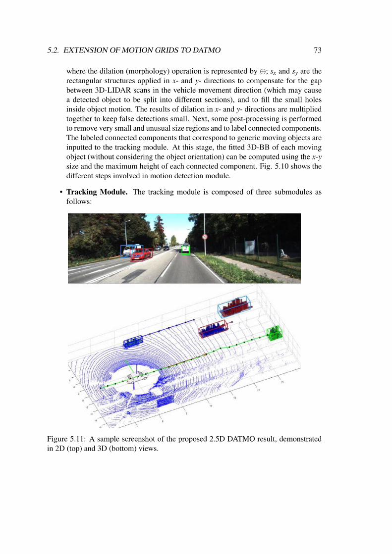
5.2. EXTENSION OF MOTION GRIDS TO DATMO 73
where the dilation (morphology) operation is represented by ⊕; sx and sy are therectangular structures applied in x- and y- directions to compensate for the gapbetween 3D-LIDAR scans in the vehicle movement direction (which may causea detected object to be split into different sections), and to fill the small holesinside object motion. The results of dilation in x- and y- directions are multipliedtogether to keep false detections small. Next, some post-processing is performedto remove very small and unusual size regions and to label connected components.The labeled connected components that correspond to generic moving objects areinputted to the tracking module. At this stage, the fitted 3D-BB of each movingobject (without considering the object orientation) can be computed using the x-ysize and the maximum height of each connected component. Fig. 5.10 shows thedifferent steps involved in motion detection module.
• Tracking Module. The tracking module is composed of three submodules asfollows:
Figure 5.11: A sample screenshot of the proposed 2.5D DATMO result, demonstratedin 2D (top) and 3D (bottom) views.

74 CHAPTER 5. OBSTACLE DETECTION
Kalman Filter (KF) The centroid of a labeled segment of the motion (see Fig.1 and Fig. 3 (c)) is considered as a detected generic moving object (alsoknown as point model representation). A KF [123] with Constant Velocitymodel (CV-KF) is used for the prediction of each object’s location in the nextframes. An individual 2D KF is associated for every new detected movingobject.
Data Association (DA) Gating and NN strategies are used to determine whichdetected object goes with which track. Initially, for each track, Gating isapplied to prune the candidates (the detected objects). If there is more thanone candidate the nearest one is associated with the track, else if there isno candidate, it is assumed that a miss detection is occurred and the KFpredicted output from previous time step is used, and a flag is sent to thetrack management for further actions.
Track Management The main objectives of the track management are track ini-tializations for new detections and removing the tracks that left the localgrid. When there is a detection that is not associated to any existing track,a new track is initialized, but the track management unit will wait for thenext frame for confirmation. If in the next frame a detection gets associatedwith that track it is confirmed as a new track, else it is considered as a falsedetection. Fig. 5.11 shows the result of the proposed 2.5D DATMO.
5.3 Fusion at Tracking-LevelObject tracking is one of the key components of a DATMO system. Although mostapproaches work only on image or LIDAR sequences, this section proposes an ob-ject tracking method using fusion of 3D-LIDAR with RGB camera data to improve thetracking function of a multisensor DATMO system.
5.3.1 Fusion Tracking OverviewConsidering sensory inputs from a camera, a 3D-LIDAR and an INS mounted on-boardthe ego-vehicle, 3D single-object tracking is defined as: given input data (RGB image,PCD, and an ego-vehicle pose) and given the initial object’s 3D-BB in the first PCD, es-timate the trajectory of the object, in the 3D world coordinate system as both ego-vehicleand object move around a scene. The conceptual model of the proposed multisensor 3Dobject tracker is shown in Fig 5.12. Object tracking starts with the known 3D-BB in thefirst scan. Next, the ground plane is estimated, and ground points are eliminated fromthe PCD. The remaining object points P are projected into the image plane and the 2Dconvex-hull (Ω) of the projected point set, P∗, is computed. The convex-hull Ω accu-rately segments object pixels from other pixels. The 3D-BB and its corresponding Ω

5.3. FUSION AT TRACKING-LEVEL 75
3D KF Fusion 3D KF Tracking
2D - 3D Projection
Initialization
in PCD
Automatic Initial.
in Image
3D MS Localization
in PCD
2D MS Localization
in Image
3D-BB
Ω
P
Cpcd
Crgb
C’rgb
C3D
Outputs the object’s:
• Trajectory
• Velocity estimation
• Predicted location
• 3D-BB in PCD
• Orientation
• 2D convex-hull in Im.
Figure 5.12: The diagram of the major pipeline of the proposed 2D/3D fusion-based 3Dobject tracking algorithm.
are used to initialize tracking in the PCD and image. In the next time-step, two Mean-Shift (MS) [124] based localizers are run individually to estimate the 2D and 3D objectpositions in the new image and PCD, respectively. An adaptive color-based MS is usedto localize the object in the image, while the localization in the PCD is performed usingthe MS gradient estimation of the object points in the 3D-BB. The 2D position of theobject in the image is projected back to 3D. KFs with a Constant Acceleration model(CA-KF) are used for the fusion and tracking of object locations in the image and PCD.The predicted object’s position and orientation are used for the initialization of the 3D-BB in the next PCD. Fig. 5.13 shows the result of the proposed algorithm. In the nextsubsections, object localization components, in the 3D PCD and 2D RGB image, aredescribed followed by the explanation of the proposed fusion and tracking approaches.
5.3.2 3D Object Localization in PCDIncoming PCDs need to be processed to remove ground points in the 3D-BB, avoidingobject model degradation.
• Removing the Ground Points. Ground points typically constitute a large por-tion of a 3D-LIDAR’s PCD. If an appropriate feature is selected and the corre-sponding Probability Density Function (PDF) computed, then the peak-value inthe PDF could be used to indicate ground points. Leveraging this fact, a KernelDensity Estimation (KDE) is used to estimate the PDF of angles (the consideredfeature) between the x-y plane and the set of lines passing through the center

76 CHAPTER 5. OBSTACLE DETECTION
Figure 5.13: Proposed object tracking method results. The bottom figure shows theresult in the 3D PCD where the 3D-BB of the tracked object is shown in blue, objecttrajectory is represented as a yellow curve and the current estimated speed of the objectis shown inside a text-box (27.3 km/h). The ego-vehicle trajectory, given by an INSsystem, is represented by a magenta curve. Parts of the 3D-LIDAR PCD in the fieldof view of the camera are shown in white (obstacle points) and red (detected groundpoints). The top figure represents the tracking result in the 2D RGB image, where thedetected object region and its surrounding area are shown in blue and red, respectively.
of the ego-vehicle (the origin point) and every point belonging to the PCD. LetΘ = θ1, · · · ,θN denote the set of 1D angle values (measured in x-z plane) for aPCD, where θi = arctan(zi / xi). The univariate KDE is obtained by
P(θ) = 1N ∑
Ni=1Kσ (θ −θi) (5.10)
where Kσ (.) is a Gaussian kernel with width σ , and N is the number of points.

5.3. FUSION AT TRACKING-LEVEL 77
ix
iz
i
the origin point
the end point i
(a)
(b)
(c)
x axis
Figure 5.14: The ground removal process. (a) The angle value θi for a point i; (b) KDEof the set Θ and the detected pitch angle θρ , and (c) The ground removal result. Redpoints denote detected ground points. The green ellipse shows the PCD of the car andthe detected points. The corresponding car in the image is shown with a red ellipse.
The ground is assumed to be plane, and the pitch angle of the ground plane isidentified as the KDE’s peak value θρ . The points below a certain height dminfrom the estimated ground plane are considered as being the ground points (Fig.5.14). In order to increase the robustness of the ground removal process, a KFwith CA model is used for the estimation of the ground plane’s pitch angle. Toeliminate outliers, the angle search area is limited to a gate in the vicinity of thepredicted KF value from the previous step. If no measurements are availableinside the gate, the predicted KF value is used.
• MS-based Localization in PCD. Object localization in the PCD is performed asfollows:
1. Computing the shift-vector. Given the center of the 3D-BB as χ , the shift-

78 CHAPTER 5. OBSTACLE DETECTION
Figure 5.15: The MS procedure in the PCD. Left: bird’s-eye view. Right: top view. Thebrighter blue color of the 3D-BB shows the most recent iteration.
vector between χ and the point set P′ inside the 3D-BB is computed using,
mk = χk−µ(P′) (5.11)
where µ(.) indicates the mean function, and k is the iteration index.
2. Translating 3D-BB. The 3D-BB is translated using the shift-vector,
χk+1 = χk +mk (5.12)
The shift-vector always points toward the direction of the maximum increasein the density.
3. Iterating steps 1 and 2 until convergence. The MS iteratively shifts the3D-BB until the object is placed entirely within the 3D-BB. A centroidmovement |mk| less than 5 cm or a maximum number of iterations equalto 5 are considered as the MS convergence.
The MS process in PCD is shown in Fig. 5.15. The object position is represented bythe centroid of object points (point model) inside the 3D-BB. The point model is feasibleeven with a few number of object points which is the case in sparse 3D-LIDAR’s PCD(especially for far objects). The centroid after convergence is denoted by Cpcd andoutputted to the fusion module.
5.3.3 2D Object Localization in ImageObject points P (after ground removal) are projected onto the image and the 2D convex-hull (also calledΩ region) of the projected point set P∗= p∗1, · · · , p∗n is computed. The

5.3. FUSION AT TRACKING-LEVEL 79
Mapping
MS Localization
(a)
2D MS Localization
in the RGB Image
Object and Background
Convex-hulls
(b)
Figure 5.16: The MS computation in the image. (a) the schematic diagram of the MScomputation work flow. (b) Left: Ω and Ω† in blue and red, respectively. Middle:computed ℜ and f. Each non-empty bin in the ℜ is represented by a circle. Eachbin-value is represented by the area of a circle. Each circle’s location represents a colorin the histogram (the same as its face color). Right: MS localization procedure. Thebrighter blue Ω indicates the most recent MS iteration.
2D convex-hull is the smallest 2D convex polygon that encloses P∗. The computed Ωaccurately segments the object from the background in comparison with the traditionalrectangular 2D-BB. The surrounding area Ω† is computed automatically by expandingΩ by a factor equal to
√2 with respect to its centroid so that the number of pixels in
Ω− =Ω†−Ω (the region between Ω and Ω†) is approximately equal to the number ofpixels within Ω.
• Color Model of the Object. Two joint RGB histograms are calculated from thepixels withinΩ andΩ− regions. The LLR of the RGB histograms expresses howmuch more likely each bin is underΩ color model thanΩ−. In the LLR, positivebins more likely belong to Ω, bins with a negative value to Ω− and bins sharedby both Ω and Ω− tend to zero. The positive part of the LLR is used to representthe discriminant object color model,
ℜ(i) = max
log maxHΩ(i),εmaxHΩ−(i),ε
, 0
(5.13)
80 CHAPTER 5. OBSTACLE DETECTION
where HΩ and HΩ− are the computed histograms from the Ω and Ω− regions,respectively; ε is a small value that prevents dividing by or taking the log of zero,and the variable i ranges from 1 to the number of histogram bins. The color modelof the object (ℜ) is normalized and used for localizing the object in the next frame.
• MS-based Localization in Image. MS-based object localization for the nextframe starts at the centroid of the confident map (f) of theΩ region in the currentframe. This confidence map is computed by replacing the color value of each pixelin the Ω region by its corresponding bin value in ℜ. In each iteration, the centerof Ω, from the previous step, is shifted to the centroid of f (current confidencemap) computed as follows:
Cnew = 1m ∑
mi=1fi Ci (5.14)
where Ci = ri,ci denotes pixel positions in Ω, and m is the total number of pix-els in Ω. The maximum number of MS iterations needed to achieve convergencewas empirically limited to 4 unless the centroid movement is smaller than a pixel(see Fig. 5.16). The computed 2D object centroid after convergence is denotedby Crgb and outputted to the fusion module.
• Adaptive Updating of ℜ Bins. RGB images obtained from cameras are veryinformative but they are very sensitive to variations in illumination conditions.To adapt the object color model and overcome changes in the object color appear-ance during tracking, a bank of 1D KFs with a CA model is applied. KFs estimateand predict ℜ bin values for next frames. A new 1D KF is initialized and associ-ated with every newly observed color bin. When the bin values become zero ornegative, the corresponding KFs are removed. Based on a series of tests where8×8×8 histograms (512 bins) were considered, the average number of utilizedKFs in each frame were about 70 (∼ 14% of the total number of bins).
5.3.4 KF-based 2D/3D Fusion and TrackingKFs are used for the fusion and tracking of object centroids obtained from the imageand the PCD:
• 2D/3D Fusion for Improved Localization. The computed 2D location of theobject (Crgb) is projected back to 3D (C′rgb) using a method described in [64].Although originally used for up-sampling a PCD, we employ it for projecting theobject centroid in the image back to the 3D-LIDAR space. The PCD is projectedinto the image and the nearest points in each of the 4 quadrants (upper left/rightand lower left/right) surrounding Crgb are found. The bilinear interpolation onthe corresponding 4 points in the PCD (before the projection to the image) iscomputed to estimate C′rgb.

5.3. FUSION AT TRACKING-LEVEL 81
A KF-based fusion (the measurement fusion model [125]) is applied to integrateC′rgb with Cpcd and estimate the fused centroid C3D. The idea is to give more trustto the method that performs better, thus providing a more accurate estimate thaneach method individually. The dynamics of the object and the fused measurementmodel of the object localizers in the PCD and image are given by
xt = AF · xt−1 +wt
zt = HF · xt + vt(5.15)
where wt and vt represent the process and measurement noise, AF is the fusionstate transition matrix, and HF is the fusion transformation matrix. The aug-mented measurement vector zt is given by,
zt =[(Cpcd)
> (C′rgb)>]>
(5.16)
• 3D Tracking. A 3D CA-KF is used for the robust tracking of the fused centroidC3D. Let the state of the filter be x =
[x,y,z, x, y, z, x, y, z
]>, where x, y, z and x, y, zdefine the velocity and acceleration corresponding to the x,y,z location. The dis-crete time process and measurement models of the system are given by
xt = AT · xt−1 +wt
zt = HT · xt + vt(5.17)
where AT and HT are the state transition matrix and the transformation matrixfor object tracking. To eliminate outliers and increase the robustness, the searcharea is limited to a gate in the vicinity of the predicted KF location (accessiblefrom: xt = AT ×xt−1). If no measurement is available inside the gate area, the KFprediction is used.
The result of the proposed algorithm is the estimated trajectory of the object in 3D worldcoordinates, its velocity, and the predicted object location in the next time-step. Objectorientation is achieved by subtracting its current and previous locations.

82 CHAPTER 5. OBSTACLE DETECTION

Chapter 6
Object Detection
Contents6.1 3D-LIDAR-based Object Detection . . . . . . . . . . . . . . . . . 84
6.1.1 DepthCN Overview . . . . . . . . . . . . . . . . . . . . . . . 84
6.1.2 HG Using 3D Point Cloud Data . . . . . . . . . . . . . . . . 84
6.1.3 HV Using DM and ConvNet . . . . . . . . . . . . . . . . . . 86
6.1.4 DepthCN Optimization . . . . . . . . . . . . . . . . . . . . . 90
6.2 Multimodal Object Detection . . . . . . . . . . . . . . . . . . . . 90
6.2.1 Fusion Detection Overview . . . . . . . . . . . . . . . . . . 91
6.2.2 Multimodal Data Generation . . . . . . . . . . . . . . . . . . 92
6.2.3 Vehicle Detection in Modalities . . . . . . . . . . . . . . . . 92
6.2.4 Multimodal Detection Fusion . . . . . . . . . . . . . . . . . 92
In the last chapter, we described the proposed methods for generic object detection byprocessing a temporal sequence of sensors’ data. This chapter addresses the problemof class-specific object detection from a single frame of multisensor data. This chapterstarts by detailing 3D object detection using 3D-LIDAR data and then proceed to de-scribing multisensor and multimodal fusion for object detection task. In this chapter weuse the ‘Car’ class as the example of class-specific object.
Parts of this chapter have been published in one journal article and 3 conferenceproceedings: Journal of Pattern Recognition Letters [126], IEEE Intelligent Trans-portation Systems Conferences [127, 128], and the Third Iberian Robotics Conference[129].
83

84 CHAPTER 6. OBJECT DETECTION
6.1 3D-LIDAR-based Object Detection
The application of an unsupervised learning technique to support (class-specific) super-vised learning based object detection was the main purpose of this section. A vehicledetection system (herein called DepthCN) based on the Hypothesis Generation (HG)and Verification (HV) paradigms is proposed. The data inputted to the system is a pointcloud obtained from a 3D-LIDAR mounted on board an instrumented vehicle, which isthen transformed to a dense-Depth Map (DM). Specifically, the DBSCAN clustering isused to extract structures (i.e., to segment individual obstacles that stand on the ground)from the 3D-LIDAR data to form class-agnostic object hypotheses, followed by (class-specific) ConvNet-based classification of such hypotheses (in the form of a DM). Theterm ‘object hypotheses’, which we use interchangeably with ‘object proposals’ refersto the projection of segmented ‘obstacles’ to the camera coordinate system.
6.1.1 DepthCN Overview
The architecture of DepthCN is presented in Fig. 6.1. The approach comprises twostages: 1) the offline learning stage to optimize HG and HV steps, 2) the online vehi-cle detection stage. After offline optimization, the optimized parameters (highlightedin Fig. 6.1) are passed to the online stage. The online detection starts with removingground points, clustering the LIDAR’s point cloud to form segmented obstacles andthen projecting the obstacles onto 3D-LIDAR-based dense-Depth Map (DM). Bound-ing boxes are fitted to the individual projected obstacles as object hypotheses (the HGstep). Finally, the bounding boxes are used as inputs to a ConvNet to classify/verify thehypotheses of belonging to the category ‘vehicle’ (the HV step).
In the following, the proposed Hypothesis Generation (HG) using 3D-LIDAR dataand Hypothesis Verification (HV) using DM and ConvNet are described, and then theoffline DepthCN optimization process is explained.
6.1.2 HG Using 3D Point Cloud Data
Objects in driving environment may appear in different sizes and locations. The state-of-the-art approaches speed-up the detection process using a set of object proposalsinstead of an exhaustive sliding windows search. In this section, vehicle proposals aregenerated solely from 3D-LIDAR data.
Grid-based Ground Removal
To increase the quality of object proposals and to reduce unnecessary computations,points that belong to the ground first need to be removed. In a grid-based framework,

6.1. 3D-LIDAR-BASED OBJECT DETECTION 85
Offline Optimization
HG Optimization
Exhaustive
Search:
ConvNet Training
Ground Rem.: 𝜈, 𝛿
Obstacle Seg.: 𝜂, 𝜖
Training Set
GT BBs
and Labels
LIDAR PCDs
ConvNet Training
Data
Augmen.
DM
Gen.
Online Vehicle Detection
Hypothesis Generation (HG)
Hypothesis Verification (HV)
3D-LIDAR
PCD Ground
Removal
Obstacle
Segmentation
3D – 2D
Projection
Proposal
BBs
Trained
ConvNet
Proposal
BBs
𝜈, 𝛿 𝜂, 𝜖
Segmented
Obstacles
Trained ConvNet and 𝜂, 𝜖, 𝜈, 𝛿
3D-LIDAR
PCD DM
Generation
Candidate
Extraction
ConvNet
Classification
Detected
Vehicles
Figure 6.1: The proposed 3D-LIDAR-based vehicle detection algorithm (DepthCN).
ground points are eliminated by rejecting cells containing points with low variance inz-dimension.
Obstacle Segmentation for HG
3D-LIDARs have previously shown promising performance for obstacle detection (sec-tion 5). Taking this into account, we explore a HG technique using data from a 3D-LIDAR. After removing ground points, by applying DBSCAN [1] on the top-view x-yvalues of the remaining points, 3D-LIDAR points are segmented into distinctive clus-ters where each cluster approximately corresponds to an individual obstacle in the en-vironment. The segmented obstacles (i.e., clusters) are then projected onto the cameracoordinate system (using LIDAR to camera calibration matrices), and the fitted 2D-BBfor each cluster is assumed as an object hypothesis (see Fig. 6.2).

86 CHAPTER 6. OBJECT DETECTION
Examples of segmented obstacles
Examples of object proposals
Figure 6.2: HG using DBSCAN in a given point cloud. Top shows the point cloudwhere the detected ground points are denoted with green and LIDAR points that are outof the field of view of the camera are shown in red. The segmented obstacles are shownwith different colors. The bottom image shows the projected clusters and HG resultsin the form of 2D-BBs (i.e., object proposals). The image frame here is used only forvisualization purpose. The right-side shows the zoomed view, and the vertical orangearrows indicate corresponding obstacles. The dashed-blue BBs indicate two vehiclesmarked by KITTI Ground-Truth (GT).
6.1.3 HV Using DM and ConvNetThe ConvNet classifier focuses on identifying vehicles from the set of object hypothesesonto 3D-LIDAR-based DM (as illustrated in Fig. 6.3). At this stage, the system encom-passes two steps: 1) DM generation from 3D-LIDAR data and 2) DM-based ConvNetfor vehicle Hypothesis Verification (HV).
DM Generation
To generate a dense (up-sampled) map from LIDAR, a number of techniques can be usedas described in [128, 130, 131]. Here, the LIDAR dense-Depth Map (DM) generationis made by projecting sparse 3D-LIDAR’s point cloud on camera coordinate system,performing interpolation and encoding as described in the sequel (see Fig. 6.4).
• 3D-LIDAR – Image Projection. 3D-LIDAR’s point cloud data P = X ,Y,Z, isfiltered to the camera’s field of view, and projected onto the 2D-image plane using
P∗ =
Projection Matrix︷ ︸︸ ︷PC2I×R0×PL2C × P, (6.1)

6.1. 3D-LIDAR-BASED OBJECT DETECTION 87
Figure 6.3: The generated dense-Depth Map (DM) with the projected hypotheses (41object proposals are depicted with red rectangles). For viewing the corresponding RGBimage and 3D-LIDAR data please refer to Fig. 6.2.
where PC2I is the projection matrix from the camera coordinate system to theimage plane, R0 is the rectification matrix, and PL2C is LIDAR to camera coor-dinate system projection matrix. Considering P∗ = X∗,Y ∗,Z∗, using the rowand column pixel values X∗,Y ∗ accompanied with range data Z∗, a compactsparse Range Map (sRM) is computed, which has a lower density than the imageresolution.
• sRM Depth Encoding. sRM is converted to 8-bit integer gray-scale image formatusing Range Inverse method which dedicates more bits to closer depth values. Letζ ∈ Z∗ be the projected real-range values, and ζmin and ζmax the minimum andmaximum range values considered. The 8-bit quantized depth-value of a pixel(ζ8bit) is attained by
ζ8bit =⌊
ζmax×(ζ−ζmin)ζ×(ζmax−ζmin)
×255⌋, (6.2)
where b.c denotes the floor function. This process converts the original rangevalues in sRM to the 8-bit quantized sparse Depth Map (sDM).
• Delaunay Triangulation (DT). We adopted the Delaunay Triangulation (DT) asa technique to obtain high-resolution maps. DT is effective in obtaining densemaps with close to 100% of density because this method interpolates all locationsin the map regardless the positions of the input (raw) points. The DT is used formesh generation from the row and column values X∗,Y ∗ of the projected 3D-LIDAR points P∗. The DT produces a set of isolated triangles ∆ = δ1, · · · ,δn,each triangle δ composed of three vertices nk,k : 1,2,3, useful for building theinterpolating function F (·) to perform an interpolation over sDM depth values.
• Interpolation of sparse Depth Map (sDM). Unsampled (missing) intensity valuei of a pixel location P which lie within a triangle δ , is estimated by interpolating

88 CHAPTER 6. OBJECT DETECTION
(a)
(b)
(c)
(d)
Figure 6.4: Illustration of the DM generation process: (a) a color image with superim-posed projected LIDAR points; (b) the generated 2D triangulation; (c) the zoomed areawithin the red box of above image, and (d) shows the constructed DM.

6.1. 3D-LIDAR-BASED OBJECT DETECTION 89
A proposal
1st
Kernel
32th
Kernel
66x112x1 input
32 Kernels 5x5x1
Stride 1, Padding 2 x
f(x)
1st Convolutional Layer 1st Max
Pooling Layer
S@2 P@0 ReLU
2nd Conv.
Layer
2nd Max
Pool. Layer
Dropout Positive
(Car)
Negative
FC FC
S@2
P@0
64@5x5x32
S@1 P@2
Figure 6.5: The ConvNet architecture (details of the second convolutional and poolinglayers are ignored to improve readability).
depth values of the surrounding triangle vertices nk,k : 1,2,3 using NearestNeighbor interpolation function F (which means selecting the value of the clos-est vertex) applying (6.3), ending up in a DM (Fig. 6.4).
i=F (argminnk‖P−nk‖), k : 1,2,3 (6.3)
ConvNet for Hypothesis Verification (HV)
ConvNet is used as the HV core in DepthCN. The ConvNet input size is set as 66×112where 66 and 112 are the average Ground-Truth (GT) vehicle height and width (in pix-els) in the training dataset. An object proposal BB in the DM is extracted as the vehiclecandidate (see ‘Candidate Extraction’ in Fig. 6.1), resized to 66× 112 and inputted toConvNet for classification. The ConvNet employed in DepthCN is composed by 2 Con-volutional layers, 3 Rectified Linear Units (ReLUs), 2 Pooling layers, 2 Fully Connected(FC) layers, a Softmax layer, and a Dropout layer for regularization (as illustrated in Fig.6.5). Each component of ConvNet architecture is described briefly in the following.
• Convolutional Layers. by applying convolution filters across input data, featuremaps are computed. The first and the second convolutional layers contain 32filters of 5×5×1 and 64 filters of 5×5×32 respectively.
• ReLUs. ReLUs use the non-saturating activation function F (x) = max(0,x),elementwise, to increase the nonlinear properties of the network. ReLUs are usedin the first and the second convolutional layers, and after the first FC layer.
• Max-Pooling. Max-pooling (with stride 2 and padding 0) is used to partitionthe input feature maps into sets of 3× 3 rectangle sub-regions. It outputs themaximum value for each sub-region.

90 CHAPTER 6. OBJECT DETECTION
• Fully-Connected (FC) layers. FC layers have full connections to all activationsin the previous layer. Two FC layers with 64 and 2 neurons are used to providethe classification output.
6.1.4 DepthCN OptimizationDepthCN’s online phase is composed by HG and HV modules (see Fig. 6.1). Theoptimization of these modules are performed offline as follows.
HG Optimization
In the grid-based ground removal, the parameters are grid cell size (υ) and variancethreshold (δ ). The minimum number of points (η) and the distance metric (ε) arerelated to DBSCAN. The optimal parameter values for ground removal and clusteringwere optimized jointly, using exhaustive search, by maximizing the overlap of generatedhypotheses with ground-truth BBs (minimum overlap of 70%).
ConvNet Training using Augmented DM Data
The ConvNet was trained on the augmented 3D-LIDAR-based DMs. Data augmentationis the process of generating a large training dataset from a small dataset using differenttypes of transformations in a way that a balanced distribution is reached, while the newdataset still resembles the distribution that occurs in practice (i.e., increasing trainingdata such that it still resembles what might happen under real-world conditions). In theproposed approach, a set of augmentation operations like scaling and depth-value aug-mentations, to resemble the closer and further objects; flipping, to simulate the effect ofdriving in the opposite direction; jittering and aspect-ratio augmentations, to simulatethe effect of potential calibration errors and inaccurate GT labeling; cropping, to resem-ble occlusions that may occur in practice; rotation, to resemble objects being at differentpositions on the road, and shifting each line with different small random biases to re-semble noise and depthmap generation errors are performed. This process is performedto aggregate and to balance the training dataset with two major goals and benefits: i)Balancing data in classes: reducing bias of ConvNet, ii) Increasing training data: help-ing ConvNets to tune large number of parameters in the network. The ConvNet trainingis performed after DM-based augmentation using Stochastic Gradient Descent (SGD)with dropout and `2 regularizations.
6.2 Multimodal Object DetectionMost of the current successful object detection approaches are based on a class of deeplearning models called Convolutional Neural Networks (ConvNets). While most exist-

6.2. MULTIMODAL OBJECT DETECTION 91
Fused
Detection
Vehicle Detectors Multimodal Detection Fusion
Color Image
DM
RM
Multimodal Data Gen.
PCD BB , s
BBR, sR
BB , s
Feature
Extraction
BB , s′
BBR, s′R
BB , s′
BBF, sF 3L
Cam.
DM Gen.
RM Gen.
YOLOv2-D
YOLOv2-R
YOLOv2-C
Joint Re-scoring
MLP N
MS
Figure 6.6: The pipeline of the proposed multimodal vehicle detection algorithm. Cam.and 3L are abbreviations for Camera and 3D-LIDAR, respectively
ing object detection researches are focused on using ConvNets with color image data,emerging fields of application such as Autonomous Vehicles (AVs) which integratesa diverse set of sensors, require the processing for multisensor and multimodal infor-mation to provide a more comprehensive understanding of real-world environment.This section proposes a multimodal vehicle detection system integrating data from a3D-LIDAR and a color camera. Data from LIDAR and camera, in the form of threemodalities, are the inputs of ConvNet-based detectors which are later combined to im-prove vehicle detection. The modalities are: (i) up-sampled representation of the sparseLIDAR’s range data called dense-Depth Map (DM), (ii) high-resolution map from LI-DAR’s reflectance data hereinafter called Reflectance Map (RM), and (iii) RGB imagefrom a monocular color camera calibrated wrt the LIDAR. Bounding Box (BB) detec-tions in each one of these modalities are jointly learned and fused by an Artificial Neu-ral Network (ANN) late-fusion strategy to improve the detection performance of eachmodality. The contribution of the proposed approach is two-fold: 1) probing and evalu-ating 3D-LIDAR modalities for vehicle detection (specifically the depth and reflectancemap modalities), and 2) joint learning and fusion of the independent ConvNet-basedvehicle detectors (in each modality) using an ANN to obtain a more accurate vehicledetection.
6.2.1 Fusion Detection OverviewThe architecture of the proposed multimodal vehicle detection system is shown in Fig.6.6. Three modalities, DM, RM (both generated from 3D-LIDAR data) and color imageare used as inputs. Three YOLOv2-based object detectors are run individually on eachmodality to detect the 2D object BBs in the color image, DM and RM. 2D-BBs obtainedin each of the three modalities are fused by a re-scoring function followed by a non-maximum suppression. The purpose of the multimodal detection fusion is to reducethe misdetection rate from each modality which leads to a more accurate detection. Inthe following, we start by describing the multimodal data generation. Next, we explain

92 CHAPTER 6. OBJECT DETECTION
the proposed multimodal fusion scheme including a brief introduction of the YOLOv2framework, which is the ConvNet-based vehicle detector considered for each modality.
6.2.2 Multimodal Data GenerationThe color image is readily available from the color camera. However, 3D-LIDAR-baseddense maps are not directly available and need to be computed. Assuming that a LIDARand a camera are calibrated with respect to each other, the projection of the LIDAR pointinto the image plane is much sparser than its associated image. Such limited spatial res-olution of the LIDAR makes object detection from sparse LIDAR data challenging.Therefore, in the proposed method, we propose to generate high-resolution (dense) maprepresentations using LIDAR data to (i) perform deep-learning-based vehicle detectionin LIDAR dense maps and, (ii) to carry out a decision-level fusion strategy. Besides thedepth map (DM), a dense reflectance map (RM) is also considered in the vehicle detec-tion system. In the case of DM, the variable to be interpolated is the range (distance),while the reflectance value (8-bit reflection return) is the variable to be interpolated togenerate the RM. LIDAR reflectivity attribute is related to the ratio of the received beamsent to a surface, which depends upon the distance, material, and the angle between sur-face normal and the ray. Fig. 6.8 shows an example color image followed by the densemaps (DM and RM) obtained using DT and nearest neighbor interpolation. The imageand the LIDAR data used to obtain the dense maps are taken from the KITTI dataset.
6.2.3 Vehicle Detection in ModalitiesYou Only Look Once (YOLO) [24, 25] is a real-time object detection system. In YOLO,object detection is defined as a regression problem and, taking advantage from a grid-based structure, object BBs and detection scores are achieved directly (i.e., without theneed for an object proposal step). In this work, the most-recent version of YOLO, de-noted as YOLOv2 [25] is used. The YOLOv2 network is composed by 19 convolutionallayers and 5 max-pooling layers. The input image (after resizing to 416×416 pixels) isdivided into 13×13 grid regions, and five centers of the BBs are assumed in each gridcell. A non-maximum suppression is applied to suppress duplicated detections (see Sec-tion 3.3 for more details). YOLOv2 is trained individually on each of the three trainingsets (color, DM and RM). The result is three trained YOLOv2 models, one per modality.
6.2.4 Multimodal Detection FusionThis section presents a multimodal detection fusion system that tries to use the associ-ated confidence of individual detections (detection scores) and the detected BBs’ char-acteristics in each modality to learn a fusion model and deal with detection limitationsin each modality.

6.2. MULTIMODAL OBJECT DETECTION 93
1
µx,µ
y
Image Plane
𝐵𝐵𝑀
2
3
4
5
Feature Extraction Target
sC sD sR BBC BBD BBR μx μy 𝜎x 𝜎y BBM
- -
- - - -
IOU IOU IOUR
- - -
- -
NN
Training 1
2
3
4
5
Figure 6.7: Feature extraction and the joint re-scoring training strategy. Some of thedifferent situations that may happen in tri-BBs generation are depicted in ‘image plane’(in the left). The detections from YOLOv2-C, YOLOv2-D, YOLOv2-R and the ground-truth are depicted, in the image plane, with red, green, blue and dashed-magenta BBs,respectively. Feature extraction and the target are represented by matrices where eachcolumn corresponds to a feature and each row a combination of detections (in the mid-dle). Each matrix cell contains the colors corresponding to the detections contributingto the feature’s value or a dash in gray background for an empty cell (zero).
Joint Re-Scoring using MLP Network
The detections from modalities are in the form of a set of BBs BBC,BBD,BBR withtheir associated confidence scores sC,sD,sR. The overlap between BBs BBC,BBD,BBRis computed and boxes that overlap are considered to be detecting the same object. Then,a set of overlapping BBs is extracted, and for each detector present in the set all com-binations are extracted (see Fig. 6.7). The ideal result is a set of three BBs (henceforthcalled tri-BBs), each from one modality. If a given modality is not present on the set,the corresponding detector BB is considered to be empty (BB=/0). A Multi-Layer Per-ceptron Neural Network is used as a fitting function and applied over a set of attributesextracted from the tri-BBs to learn the multi-dimensional nonlinear mapping betweenthe BBs from modalities and the ground-truth BBs. For each combination of BBs the

94 CHAPTER 6. OBJECT DETECTION
attributes extracted (F) are as follows:
F = (sC,sD,sR,BBC,BBD,BBR,µx,µy,σx,σy,BBM), (6.4)
where sC, sD, sR are the detection confidence scores and BBC, BBD, BBR are the BBscorrespondent to the color, DM and RM detectors. Every BB is defined by four prop-erties w,h,cx,cy which indicate width, height and the geometrical center in x and y(all normalized with respect to the image’s width and height), respectively. The µx, µy,σx, and σx correspond to the average of all available BBs geometrical centers and theirstandard deviation. BBM corresponds to the minimum bounding box that contains allnon empty bounding boxes in the combination. In cases where combinations do notcontain one or two detectors, scores and BBs for those detectors are set to zero and arenot included in the computation of the average, standard deviation and minimum con-taining bounding box (see Fig. 6.7). This results in a feature vector size of 23. Theassociated set of target data (T), defining the desired output, is determined as a set ofthree intersection-over-union (IOU) metrics:
T = (IOUC, IOUD, IOUR), (6.5)
IOUi =Area(BBi∩BBG)
Area(BBi∪BBG), (6.6)
where i determines each modality C,D,R and the superscript G denotes the ground-truth BB. Once the MLP has fit the data, it forms a generalization of ‘extracted featuresfrom tri-BBs’ and their ‘intersection-over-union overlap with the ground-truth’. Thetrained MLP learns to estimate the overlap of tri-BBs with the ground-truth and basedon those re-scores tri-BBs.
A simple average rule of the scores are applied when there are multiple scores forthe same BB. The re-scoring function generates, per frame, the same set of detectionBBs from different modalities i.e., BBC,BBD,BBR with the re-scored detection confi-dences s′C,s′D,s′R (see Fig. 6.6).
Non-Maximum Suppression
The input to the Non-Maximum Suppression (NMS) module is the set of BBs in thesame ‘neighborhood’ area which is a consequence of having a multimodal detection sys-tem. This could degrade the performance of the detection algorithm, as can be seen lateron in the experimental results section. To solve this, NMS is used to discard multiple-detected occurrences around close locations i.e., to retain the local most-confident de-tector. The ratio Υ between the intersection and the union area of the overlappingdetection windows is calculated and for Υ > 0.5 (value obtained experimentally) thedetection window with the greatest confidence score is retained and the remaining de-tections are suppressed. Further strategies to perform NMS are addressed by Franzel etal. [132]. An example of the fusion detection process is shown in Fig. 6.8.

6.2. MULTIMODAL OBJECT DETECTION 95
(a) 0.470.4
0.32
(b)0.33 0.3 0.43 0.55
0.78
(c) 0.570.72
(d) 0.470.4
0.320.33 0.3 0.43 0.55
0.78
0.570.72
(e) 0.480.32
0.130.05 0.07 0.39
0.350.17
Figure 6.8: Illustration of the fusion detection process: (a) detections from YOLOv2-C(red); (b) YOLOv2-D (green), and (c) YOLOv2-R (blue) with associated confidencescores; (d) represents the merged detections, and (e) shows the fusion vehicle detectionresults (cyan) after re-scoring and NMS compared to ground-truth (dashed-magenta). Adashed cyan BB indicates detections with confidence less than 0.2 that can be discardedby simple post-processing.

96 CHAPTER 6. OBJECT DETECTION

Chapter 7
Experimental Results and Discussion
Contents7.1 Obstacle Detection Evaluation . . . . . . . . . . . . . . . . . . . . 97
7.1.1 Static and Moving Obstacle Detection . . . . . . . . . . . . . 97
7.1.2 Multisensor Generic Object Tracking . . . . . . . . . . . . . 106
7.2 Object Detection Evaluation . . . . . . . . . . . . . . . . . . . . . 111
7.2.1 3D-LIDAR-based Detection . . . . . . . . . . . . . . . . . . 111
7.2.2 Multimodal Detection Fusion . . . . . . . . . . . . . . . . . 113
In this chapter we describe the experiments carried out to evaluate the proposed obsta-cle and object detection algorithms using the KITTI dataset. Comparative studies withother algorithms were performed whenever it was possible.
7.1 Obstacle Detection EvaluationThe obstacle detection performance assessment is consists of the evaluation of the pro-posed ground estimation; stationary and moving obstacle detection and segmentation;2.5D grid-based DATMO, and the proposed fusion tracking algorithms. These algo-rithms were previously described in Chapter 5.
7.1.1 Static and Moving Obstacle Detection
In this subsection we describe the evaluation of the proposed ground surface estimationand the stationary – moving obstacle detection methods. The parameter values used in
97

98 CHAPTER 7. EXPERIMENTAL RESULTS AND DISCUSSION
Table 7.1: Values considered for the main parameters used in the proposed obstacledetection algorithm.
m η τ° ` dmin υ Td Ts
6 6 10 10 20 10 5 50
the implementation of the proposed algorithm are reported in Table 7.1. The first pa-rameter m is a general parameter indicating the number of merged scans. The next fourparameters, (η , τ°, ` and dmin) are related to the ground surface estimation: η showsthe number of ∆α used to compute each slice limits; τ° and ` are respectively the max-imum acceptable angle and distance between two the planes applied in the validationphase of the piecewise plane fitting. The parameter dmin is a threshold in centimeters.Points with heights lower than dmin from the piecewise planes are considered as partof the ground plane. The last three parameters (υ , Td and Ts) are used to configurethe obstacle detection algorithm: υ is the voxel size in centimeters, and Td and Ts arethresholds for computing the binary mask of stationary and moving voxels. The pro-posed approach detects obstacles in an area covering 25 meters ahead of the vehicle, 5meters behind it and 10 meters on the left and right sides of the vehicle, with 2 metersin height. Parameters m and η were selected experimentally as described in the nextsubsection.
mDE0.08
2
24
0.09
4
no. of integrated scans (m)
6
no. of ∆α interval (η)
6
TA
DE
8 8
0.1
10 10
0.11
Figure 7.1: Evaluation of the proposed ground estimation algorithm in term of mDE byvarying the number of integrated scans m and parameter η (related to the slice sizes).

7.1. OBSTACLE DETECTION EVALUATION 99
Evaluation of Ground Estimation
For the evaluation of the ground estimation process, inspired by [58], we assume thatall objects are placed on the same surface as the vehicle and that the base points ofthe GT 3D-BBs (available in the KITTI dataset), are located on the real ground surface(see Section 3.2.2 and Fig. 3.3). The ground estimation error is calculated by takingthe average distance from the base points of the GT 3D-BBs to the estimated groundsurface. Concretely, the mean of Displacement Errors (mDE) in the i-th frame is definedby
mDE(i) = 1M ∑
Mk=1 |(
−−−−→pG
k − p ) · n| (7.1)
where pGk denotes the base of the GT 3D-BB of the k-th object; M is the total number of
objects in the i-th frame; the variables p and n are the point and the unit normal vectorthat define the corresponding surface plane, respectively. The mDE for all sequences iscomputed by
mDE = 1N ∑
Ni=1 mDE(i) (7.2)
where i ranges from 1 to the total number of frames in all 8 sequences of Table 3.1. ThemDE was computed for different number of integrated frames m and η . The results arereported in Fig. 7.1. The minimum mDE = 0.086 is achieved by the combination ofm = 6 and η = 6.
Evaluation of Stationary – Moving Obstacle Detection
The obstacle detection evaluation using 3D-LIDAR is a challenging task. To the best ofour knowledge, there is no available dataset with Ground-Truth (GT) for ground estima-tion or general obstacle detection evaluations1. The closest work to ours is presented in[52], where their evaluation for obstacle detection is carried out according to the numberof missed and false obstacles, determined by a human observer. We followed a similarapproach for evaluating the proposed obstacle detection system (also see Section 3.2.2).A number of 200 scans (25 scans for each sequence) were selected randomly out ofthe more than 2300 scans available on the dataset (see Table 3.1). An evaluation wasperformed for the general obstacle detection and another one for the moving obstacledetection (see Fig. 7.2).
• General Obstacle Detection Evaluation. For evaluating the general obstacledetection, voxel grids of the stationary and moving obstacles are projected intothe corresponding image, and a human observer performs a visual analysis interms of ‘missed’ and ‘false’ obstacles. It should be noticed that every distinctelement identified above the terrain level is considered as an obstacle (e.g., pole,tree, wall, car and pedestrian). The total number of missed obstacles is 186 out
1The benchmarks usually provide specific object classes e.g., pedestrians, vehicles.

100 CHAPTER 7. EXPERIMENTAL RESULTS AND DISCUSSION
Figure 7.2: An example of the obstacle detection evaluation. Red and green voxels showresults of the proposed method. The 3D-BBs of stationary and moving obstacles areshown in red and green, respectively. Only green boxes are considered for the evaluationof the moving obstacle detection algorithm performance. Blue arrows show two missedobstacles (thin and small poles).
Table 7.2: Results of the evaluation of the proposed obstacle detection algorithm.
Seq. # of Obst.Obst. Mov.
# of Missed Obst.Obst. Mov.
# of False Obst.Obst. Mov.
(1) 501 59 83 0 0 4(2) 288 28 56 0 0 7(3) 281 61 24 1 0 9(4) 381 94 10 2 0 0(5) 254 83 1 0 7 0(6) 791 551 9 0 37 8(7) 336 215 1 0 46 2(8) 179 110 2 0 0 1Total 3011 1201 186 3 90 31
of 3,011. The total number of false detected obstacles is 90. Table 7.2 reports thedetails of the obstacle detection results for each sequence. The highest number ofmissed obstacles occurs in sequences (1) and (2) that contain many thin and smallpoles. Most of the false detections happen in sequences (6) and (7) that containslowly moving objects. Some parts of very slowly moving objects may have beenseen several times in the same voxels and therefore, may wrongly be integratedinto the static model of the environment. The shadow of the wrongly modeledstationary obstacle stays for a few scans and causes the false detection.
• Moving Obstacle Detection Evaluation. The proposed obstacle detection methodis able to discriminate moving parts from the static map of the environment.Therefore, we performed an additional evaluation for measuring the performanceof the moving obstacle detection. Among the 1201 moving obstacles present in

7.1. OBSTACLE DETECTION EVALUATION 101
Table 7.3: Percentages of the computational load of the different steps of the proposedsystem: (a) dense PCD generation, (b) piecewise ground surface estimation, (c) ground -obstacle separation and voxelization, and (d) stationary - moving obstacle segmentation.
(a) (b) (c) (d)83.2% 7.1% 7.7% 2%
the considered scans, only 3 moving obstacles were missed. A number of 31 ob-stacles were wrongly labeled as moving, mainly due to localization errors. Local-ization errors cause thin poles, observed in different locations by the ego-vehicle’sperception system, to be wrongly considered as moving obstacles. The result foreach sequence is also shown in Table 7.2.
Computational Analysis
The experiments reported in this section were conducted on the first sequence of the Ta-ble 3.1, using a quad-core 3.4 GHz processor with 8 GB RAM under MATLAB R2015a.
• Processing load of the different steps. In order to evaluate what steps of thealgorithm are more time consuming, the percentages of the processing loads ofthe different phases are reported in Table 7.3. The first stage is the most compu-tationally demanding part of the algorithm, mostly because of the ICP algorithm(consuming 83.2% of the computational time). Piecewise ground surface estima-tion and ground - obstacle separation modules are accounted for 14.8% of totalcomputational time.
• Main factors affecting the computational cost. The computational cost of theproposed method depends on the size of the local grid, the size of a voxel, thenumber of integrating scans, and the number of non-empty voxels (this is becauseonly non-empty voxels are indexed and processed). The considered evaluationscenario has in average nearly 1% non-empty voxels. The size of a voxel and thenumber of integrating PCDs are two key parameters that have a correspondencewith the spatial and temporal properties of the proposed algorithm, and have di-rectly impact on the computational cost of the method. The average speed of theproposed algorithm (in frames per second) wrt the voxel size and the number ofintegrating PCDs are reported in Fig. 7.3. As it can be seen, the number of in-tegrated scans has the greatest impact on the computational cost of the proposedmethod. The proposed method configured with the parameters listed in Table 7.1works at about 0.3 fps.
• The accuracy and the computational cost. There is a compromise betweenthe computational cost versus the detection performance of the proposed method.
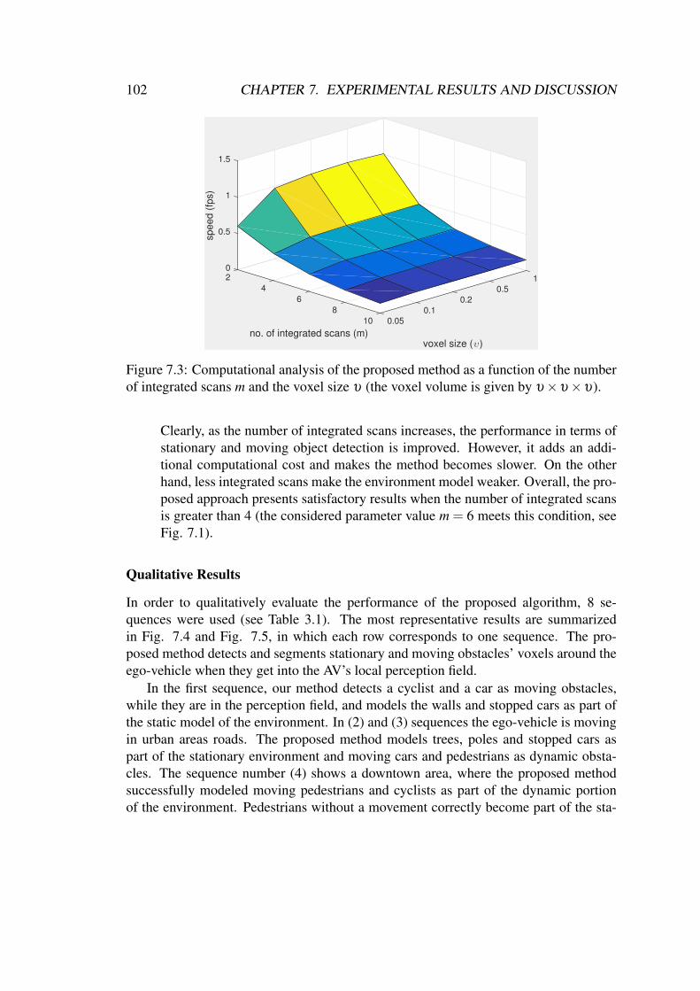
102 CHAPTER 7. EXPERIMENTAL RESULTS AND DISCUSSION
02 1
0.5
4 0.5
sp
ee
d (
fps)
1
no. of integrated scans (m)voxel size (υ)
6 0.2
1.5
8 0.1
10 0.05
Figure 7.3: Computational analysis of the proposed method as a function of the numberof integrated scans m and the voxel size υ (the voxel volume is given by υ×υ×υ).
Clearly, as the number of integrated scans increases, the performance in terms ofstationary and moving object detection is improved. However, it adds an addi-tional computational cost and makes the method becomes slower. On the otherhand, less integrated scans make the environment model weaker. Overall, the pro-posed approach presents satisfactory results when the number of integrated scansis greater than 4 (the considered parameter value m = 6 meets this condition, seeFig. 7.1).
Qualitative Results
In order to qualitatively evaluate the performance of the proposed algorithm, 8 se-quences were used (see Table 3.1). The most representative results are summarizedin Fig. 7.4 and Fig. 7.5, in which each row corresponds to one sequence. The pro-posed method detects and segments stationary and moving obstacles’ voxels around theego-vehicle when they get into the AV’s local perception field.
In the first sequence, our method detects a cyclist and a car as moving obstacles,while they are in the perception field, and models the walls and stopped cars as part ofthe static model of the environment. In (2) and (3) sequences the ego-vehicle is movingin urban areas roads. The proposed method models trees, poles and stopped cars aspart of the stationary environment and moving cars and pedestrians as dynamic obsta-cles. The sequence number (4) shows a downtown area, where the proposed methodsuccessfully modeled moving pedestrians and cyclists as part of the dynamic portionof the environment. Pedestrians without a movement correctly become part of the sta-

7.1. OBSTACLE DETECTION EVALUATION 103
(1)
(2)
(3)
(4)
Figure 7.4: A few frames of obstacle detection results obtained for sequences 1 to 4 aslisted in Table 3.1 and its corresponding representation in three dimensions. Piecewiseground planes are shown in blue. Stationary and moving voxels are shown in green andred respectively. Each row represents one sequence. From left to right we see the resultsobtained in different time instants.
tionary model of the environment. Sequence number (5) shows a crosswalk scenario.Our method models passing pedestrians as moving objects, represented in the image bygreen voxels. In sequences number (6) and (7), the vehicle is not moving. Most of themoving objects are pedestrians which our method successfully detects. In particular,

104 CHAPTER 7. EXPERIMENTAL RESULTS AND DISCUSSION
(5)
(6)
(7)
(8)
Figure 7.5: A few frames of obstacle detection results obtained for sequences 5 to 8 aslisted in Table 3.1 and its corresponding representation in three dimensions. Piecewiseground planes are shown in blue. Stationary and moving voxels are shown in green andred respectively.
notice the last image of sequence number (6) and the first image of sequence number(7) which represent very slowly moving pedestrians that may temporarily be modeledas stationary obstacles, which will not be critical in practical applications. Notice thecurvature of the ground surface in sequence number (7) that is not possible to be mod-eled using just one plane. Sequence number (8) shows a road with moving vehicles.

7.1. OBSTACLE DETECTION EVALUATION 105
Table 7.4: Values considered for the main parameters used in the proposed 2.5D grid-based DATMO algorithm.
υ Tσ Tµ n m k ε α
20 2 30 50 30 3 5 0.2
The proposed method performs well on most of the moving vehicles. When vehiclesare stopped in the traffic, they gradually become part of the static model of the environ-ment.
Extension to DATMO
In this subsection, qualitative analysis of the grid-based DATMO system is performed.The main parameter values used in the implementation of the 2.5D DATMO algorithmare reported in Table 7.4. The parameters υ , Tσ and Tµ are related to the Elevation gridgeneration: the grid resolution υ (in x-y dimensions) is chosen to be equal to 20 cm, andTσ and Tµ are the variance and height thresholds for an Elevation grid’s cell, learnedempirically. The n, m, and k are the parameters for the short-term map generation. Thespatial ε and height α parameters are linked to the motion detection module. Morespecifically, the set of all cells that lie at the (spatial) distance ε cells from the j-th cellare considered for motion detection in the j-th cell (see Fig. 5.9). The α threshold isused to calculated Te( j) = α ×E( j), which is the maximum acceptable difference ofcells’ height values. Notice that E( j) is the height value in the j-th cell. In this work,the radius ε was considered as being of 5 cells, which is a sufficient number of cells tocompensate for a maximum localization error of 1 m. The coefficient α can take a rangeof values from 0.2 to 0.5.
To the best of our knowledge, there is no standard dataset available to evaluate aDATMO approach, which is why in this section a qualitative evaluation is performed.A variety of challenging sequences were used. The most representative sequences aresummarized in Fig. 7.6. This figure is composed of two kinds of representations: theRGB image of the scene and the grid representation of the scene. The 2.5D motion grid,3D-BBs and tracks of the moving objects are shown in the grid representation. The bluedots correspond to the 3D-LIDAR PCDs and vectors on the center of the local grid showthe pose of the vehicle. Only the 3D-BB of detected moving objects are shown in theRGB image. The selected sequences are: (1) vehicles circulating on a highway; (2) aroad junction scenario, and (3) a crossing scenario.
In the first scenario, the proposed DATMO system detects and tracks all the movingvehicles when they get into the local perception field. In the road junction scenario, inthe early frames a vehicle comes from different lane and in the next frames two vehiclesjoin to the road. Our method successfully detects all moving objects. In the crossingscenario, the proposed DATMO system successfully detected the vehicles passing by.

106 CHAPTER 7. EXPERIMENTAL RESULTS AND DISCUSSION
(1)
(2)
(3)
Figure 7.6: 2.5D grid-based DATMO results of 3 typical sequences. Each row rep-resents one sequence. From top to bottom, results for: (1) vehicles circulating on ahighway; (2) a road junction scenario, and (3) a crossing scenario. Left to right we seethe results obtained in different time instants.
7.1.2 Multisensor Generic Object Tracking
In this section, we present the evaluation of the proposed multisensor 3D single-objecttracking approach. The parameter values used in the proposed fusion tracking imple-mentation are reported in Table 7.5; where η and η ′ are the maximum numbers ofMean Shift (MS) iterations in the PCD and image domains, respectively; a displace-ment δ` < 5 cm in the PCD and δ`′ < 1 pixel in the image are considered for the MSconvergence; the value dmin is the threshold in cm for the ground removal process, andb = 8 is the number of histogram bins for each color channel.
The proposed high-level fusion method (H-Fus.) was evaluated against five trackingmethods on our KITTI-based derived dataset (see Section 3.1.3 and Table 3.2). Theselected methods operate on the image or PCD or their fusion. Two image-based MSvariants: (1) The original MS [133] and (2) MS with Corrected Background WeightedHistogram (CBWH) [134]. Three PCD-based methods: (3) Baseline KF-based track-

7.1. OBSTACLE DETECTION EVALUATION 107
Table 7.5: Values considered for the main parameters used in the proposed 3D fusiontracking algorithm.
η η ′ δ` δ`′ dmin b5 4 5 1 20 8
ing that uses the ‘point model’ and 3D CA-KF with a Gating Data Association (DA);(4) MS-based object detection and localization in 3D-PCD, and (5) A low-level fusionapproach (L-Fus.) that uses MS on the colored PCD (obtained by combining PCD andRGB data), and a CA-KF. The MS-I, CBWH, KF, MS, and L-Fus. are abbreviationsfor methods (1) to (5) respectively, in Table 7.6 and Table 7.7. KF and MS methodsare further described in Appendix A. To assess the proposal’s performance, the object’scenter position errors in 2D and 3D and the object orientation error in x-y plane wereevaluated.
Evaluation of Position Estimation
The Euclidean distance of the center of the computed 2D-BB or 3D-BB from the 2D/3DGround-Truth (GT) (extracted from the KITTI dataset) are given by
E2D =1N
N
∑i=1
√(ri− rG
i )2 +(ci− cG
i )2
E3D =1N
N
∑i=1
√(xi− xG
i )2 +(yi− yG
i )2 +(zi− zG
i )2
(7.3)
where ri,ci shows the detected object position (2D-BB center); xi,yi,zi indicates thecenter of the 3D-BB in the PCD; rG
i ,cGi and xG
i ,yGi ,z
Gi denote the GT, and N is the
total number of scans. Table 7.6 summarizes the evaluation results. A dash entry (–)represents a failure of the given algorithm to track the object. The MS provides thesmallest error when it does not fail. However it is prone to errors mostly because itstarts diverging to nearby objects or obstacles in cluttered environments. The proposedmethod is the only one with stable results while keeping the center position error low.The MS-I and CBWH methods are very fragile as essentially they are not designed toovercome challenging factors in real-world driving environments (see Table 3.2).
Evaluation of Orientation Estimation
The GT orientation of the each object is given only in terms of Yaw angle which de-scribes the object’s heading (i.e., rotation around y-axis in camera coordinates in theKITTI dataset [135]). For the 3D approach, the orientation error was computed by
Eϕ = 1N ∑
Ni=1
∣∣∣arctan |−→ϕi×−→ϕi
G−→ϕi ·−→ϕi G |
∣∣∣ (7.4)

108 CHAPTER 7. EXPERIMENTAL RESULTS AND DISCUSSION
Table 7.6: Average object’s center position errors in 2D (pixels) and 3D (meters).
Seq. The Average Errors in 3D The Average Errors in 2DH-Fus. KF MS L-Fus. H-Fus. KF MS L-Fus. MS-I CBWH
(1) 0.30 – 0.21 0.25 9.2 – 8.4 11.7 263.6 298.1(2) 1.98 17.69 1.84 – 12.0 407.1 15.1 – 208.3 306.1(3) 1.67 – 1.54 1.62 3.9 – 7.2 8.6 16.3 37.5(4) 0.39 – – – 5.7 – – – 217.8 333.1(5) 0.22 2.90 0.18 1.44 12.4 157.0 12.1 53.6 279.0 128.9(6) 0.19 – 0.11 0.15 13.6 – 10.2 15.8 420.6 418.7(7) 0.26 2.30 0.19 0.18 19.5 186.9 16.3 14.5 118.8 192.6(8) 0.17 0.82 0.15 0.20 22.8 51.2 17.1 25.8 225.0 162.1
Table 7.7: Orientation estimation evaluation (in radian)
Seq. H-Fus. KF MS L-Fus.(1) 0.41 – 0.39 0.39(2) 0.41 1.25 0.42 –(3) 0.11 – 0.13 0.14(4) 0.10 – – –(5) 0.20 0.56 0.13 0.24(6) 0.20 – 0.14 0.16(7) 0.26 0.92 0.15 0.16(8) 0.15 0.29 0.14 0.15
where −→ϕ Gi is the object’s GT orientation. As it can be seen from Table 7.7, the most
stable results are provided using the proposed H-Fus. method. Similar to the pose esti-mation evaluation, the MS provides the smallest error. However, as stated before, MSis error-prone (i.e., suffers from diverging to the nearby clutters). The proposed H-Fus.approach compensates this type of error by using KFs in the fusion and tracking frame-work. A further analysis in terms of the object pose variations, and other challenges arepresented in the qualitative results section.
Computational Analysis
The experiments were performed using a quad-core 3.4 GHz processor with 8 GB RAMunder MATLAB R2015a. The non-optimized implementation of the proposed methodruns at about 4 fps. The major computational cost is due to the bank of 1D KFs whichkeeps track of the object color histogram (see Subsection 5.3.3 for details).
Qualitative Results
Results obtained by the proposed algorithm are shown in Fig. 7.7 and Fig. 7.8. Theproposed method successfully tracks the objects throughout the considered sequences.

7.1. OBSTACLE DETECTION EVALUATION 109
(1)
Frame #28/154 Frame #73/154 Frame #153/154
(2)
Frame #9/154 Frame #84/154 Frame #126/154
(3)
Frame #6/373 Frame #87/373 Frame #217/373
(4)
Frame #6/41 Frame #20/41 Frame #35/41
Figure 7.7: Object tracking results obtained for sequences 1 to 4 as listed in Table3.2 and its corresponding representation in the 3D space. In the image, blue and redpolygons denote the detected object region and its surrounding area. In the PCD, objecttrajectory is represented with a yellow curve, the 3D-BB is shown in blue and the GT3D-BB in red. The detected ground points are shown in red. Each row represents onesequence. From left to right we see the results obtained in different time instants.
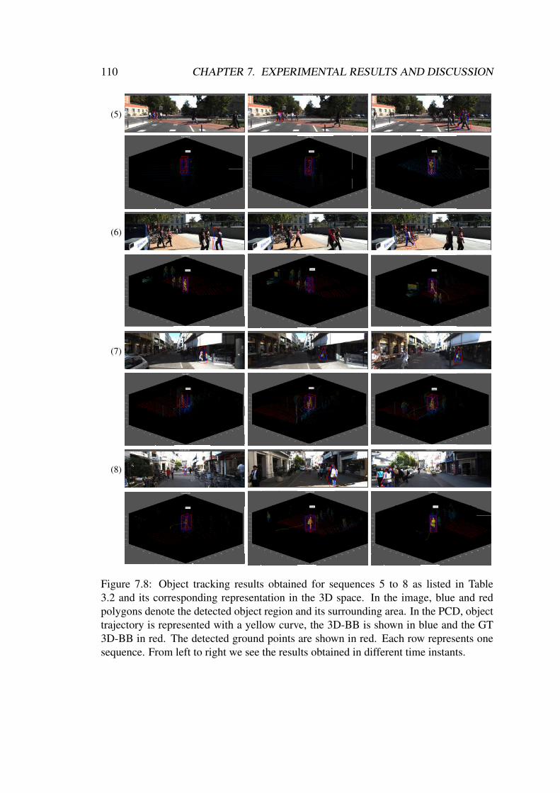
110 CHAPTER 7. EXPERIMENTAL RESULTS AND DISCUSSION
(5)
Frame #38/170 Frame #55/170 Frame #153/170
(6)
Frame #26/63 Frame #30/63 Frame #54/63
(7)
Frame #2/71 Frame #20/71 Frame #40/71
(8)
Frame #221/387 Frame #291/387 Frame #383/387
Figure 7.8: Object tracking results obtained for sequences 5 to 8 as listed in Table3.2 and its corresponding representation in the 3D space. In the image, blue and redpolygons denote the detected object region and its surrounding area. In the PCD, objecttrajectory is represented with a yellow curve, the 3D-BB is shown in blue and the GT3D-BB in red. The detected ground points are shown in red. Each row represents onesequence. From left to right we see the results obtained in different time instants.

7.2. OBJECT DETECTION EVALUATION 111
Next qualitative evaluations are presented in terms of occlusion, illumination, velocity,pose and size variations.
• Occlusion. In sequences (2) the tracked car goes under occlusion caused by aparked van. In (5) and (6) the pedestrians are occluded by other pedestrians. In(7) the pedestrian was occluded by bushes for a number of frames.
• Illumination Variations. In (1-3), and (6-8) the tracked objects go through illu-mination changes.
• Velocity Variations. In sequences (2), (3) and (8) the object of interest moveswith an unsteady velocity throughout the sequence. In sequence (3) the red caraccelerates and then stops at a crossroad and a crosswalk.
• Pose and Size Variations. In (2), (3) and (8) large variations in the object sizeoccur mostly because the distance to the ego-vehicle is changing. Object posealso varies in almost all sequences.
7.2 Object Detection Evaluation
Quantitative and qualitative experiments using ‘Object Detection Evaluation’ from KITTIVision Benchmark Suite [23] were performed to validate the performance of the pro-posed DepthCN and multimodal object detection system. Please refer to Sections 3.1.2and 3.2.2 for details of the ‘Object Detection Evaluation’ dataset and the evaluationmetrics, respectively. During the experiments, only the ‘Car’ label was considered forevaluation.
7.2.1 3D-LIDAR-based Detection
In this section we present the evaluation of DepthCN. The proposed DepthCN is relyingon Velodyne LIDAR (range data only). The maximum range in DepthCN algorithm islimited to 80 m (specifically, this value is used for generating the DM). The originalKITTI training dataset was divided into two sets: training (80%) and validation (20%),and DepthCN was optimized for the latter training and validation data. We considereddepth map as a grayscale image and employed LeNet-5 [19] (which is designed for char-acter recognition from grayscale images) with some slight modifications as the ConvNetarchitecture. DepthCN was evaluated in terms of classification and detection accuracyand computational cost. Results are provided in the next subsections.

112 CHAPTER 7. EXPERIMENTAL RESULTS AND DISCUSSION
Table 7.8: The ConvNet’s vehicle recognition accuracy with (W) and without (WO)applying data augmentation (DA).
Dataset WO-DA W-DATraining set 92.83% 96.02%Validation set 86.69% 91.93%
Table 7.9: DepthCN vehicle detection evaluation (given in terms of average precision)on KITTI test-set.
Approach Easy Moderate HardDepthCN 37.59 % 23.21 % 18.01 %
mBoW [105] 36.02 % 23.76 % 18.44 %
Evaluation of Recognition
The ConvNet training is performed after 3D-LIDAR DM-based data augmentation (seeSubsection 6.1.4). The Stochastic Gradient Descent (SGD) with a mini-batch size of128, a momentum of 0.9, and max epochs of 40 with 50% dropout and `2 regularizationwas employed for the ConvNet training. Considering an input DM of size 66×112, theaccuracy of the implemented ConvNet for vehicle classification with and without dataaugmentation is reported in Table 7.8. The data augmentation improved the accuracyby more than 5 percentage points.
Evaluation of Detection
DepthCN was evaluated against mBoW [105] which is one of the most relevant meth-ods and like ours operate directly on 3D-LIDAR’s range data. Both methods try tosolve (class-specific) object detection problem by assuming a middle cluster represen-tation that is approximately correspond to the individual obstacles that stand on theground (in practice, the segmented obstacles in LIDAR data can be used for free spacecomputation to avoid collisions). The mBoW uses hierarchical segmentation with bag-of-word classifiers whereas DepthCN uses DBSCAN with a ConvNet classifier. Resultsfor vehicle detection are given in terms of average precision (AP) in Table 7.9. As canbe noted from the table, DepthCN surpasses by about 1.5 percentage points the mBoWin Easy difficulty level, while slightly underperforms in Moderate and Hard levels. APrecision-Recall curve is shown in Fig. 7.9.
Computational Analysis
The experiments with DepthCN were performed using a Hexa core 3.5 GHz processorpowered with a GTX 1080 GPU and 64 GB RAM under MATLAB R2017a. The run-

7.2. OBJECT DETECTION EVALUATION 113
0
0.2
0.4
0.6
0.8
1
0 0.2 0.4 0.6 0.8 1
Pre
cis
ion
Recall
Car
EasyModerate
Hard
Figure 7.9: Precision-Recall on the KITTI testing dataset for easy, moderate and hardCar detection difficulty levels.
time of DepthCN (unoptimized implementation) for processing a point cloud is about2.3 seconds in comparison with 10 seconds processing time of mBoW (implemented inC/C++) under 1 core 2.5 Ghz.
Qualitative Results
Qualitative results are also provided in Fig. 7.10. The proposed method detects allobstacles (generic objects) in the environment (in the form of object proposals, as shownby red rectangles in Fig. 7.10), and then classifies the target class of object (i.e., Carclass). As it can be seen the 3D PCD of each generic object is retrievable from the3D-LIDAR’s PCD as well. It is observed that the proposed method performs better forcloser objects.
7.2.2 Multimodal Detection FusionThe dataset was partitioned into three subsets: 60% as training set (4489 observations),20% as validation set (1496 observations), and 20% as testing set (1496 observations).The experiments were carried out using a Hexa-core 3.5 GHz processor, powered witha GTX 1080 GPU and 64 GB RAM. The YOLOv22 416×416 detection framework[25] was used in the experiments. The YOLOv2 detector in each color, DM and RM
2https://pjreddie.com/darknet/yolo/

114 CHAPTER 7. EXPERIMENTAL RESULTS AND DISCUSSION
Figure 7.10: Few examples of DepthCN detection results (four pairs of DM and colorimages with corresponding PCDs). The generated hypotheses and the detection resultsare shown, in both DM and color images, as red and dashed-green BBs, respectively.The bottom figures show the result in the PCD, where the detected vehicles’ clusters areshown in different colors, and the remaining LIDAR points are shown in green. Noticethat color-images are presented just for improving visualization and making understand-ing of the results easier.
modality (referred as YOLOv2-C, YOLOv2-D and YOLOv2-R respectively) and theproposed learning-based fusion scheme were optimized using training and validationsets, and evaluated on the testing set. Pre-trained ConvNet convolutional weights, com-

7.2. OBJECT DETECTION EVALUATION 115
puted on the ImageNet dataset3, were used as initial weights for training. Each individ-ual YOLOv2-C/D/R was fine-tuned for 80200 iterations using SGD with learning rateof 0.001, 64 as batch size, weight decay of 0.0005 and momentum of 0.9. MLPs (withone and two hidden layers) were experimented for function fitting. The MLP fittingfunction was trained using Levenberg-Marquardt back-propagation algorithm.
To evaluate the proposed learning-based fusion detection method, the performanceof the fusion model with two sets of features: 1) using the confidence score featuresubset, and 2) using the entire feature set was evaluated in our offline testing set. Inaddition, we presented results in comparison with state-of-the-art methods on the KITTIonline benchmark.
Evaluation on Validation Set
The YOLOv2 vehicle detection performance for each modality (color, DM, and RMdata) is presented in Fig. 7.11. To have fair comparison among modalities, the images(DM, RM and color image) were converted to JPEG files with 75% compression quality.The average file size for each DM, RM and color modalities is approximately 28 KB,44 KB and 82 KB, respectively. As can be seen by comparing precision-recall curves,in addition to color data, the DM and RM modalities, when used individually, shownvery promising results (further analysis on RM is presented in Appendix B). Two setsof experiments were conducted for evaluating the performance of the fusion vehicledetection system. The first set of experiments demonstrates the improvement gainedusing the confidence score feature subset. In the second experiment, the entire featureset is employed for learning the joint re-scoring function.
• Experiment using the confidence score feature subset. The re-scoring functioncan be interpreted as a three-class function-fitting MLP. To visualize the perfor-mance of the fitting function, in the first experiment a 3-layer MLP is trained usinga subset of features (three detection confidence scores sC,sD,sR). All combina-tions of confidence scores are generated and inputted to the trained MLP, and theestimated intersection-over-union overlaps are computed as shown in Fig. 7.12.This figure illustrates how modality detectors are related, and shows the learnedobject detector behaviors in modalities based on the detection scores. In fact itshows in which combination of scores each detector contributes more for the finaldecision. The 3-layer MLP reached the minimum Mean Squared Error (MSE) of0.0179 with 41 hidden neurons. The Average Precision (AP) of the first exper-iment on the test set is reported in Table 7.10. The results show that the fusionmethod achieves an improved performance even when just the detection scoreswere considered.
3www.image-net.org

116 CHAPTER 7. EXPERIMENTAL RESULTS AND DISCUSSION
(a)
0 0.2 0.4 0.6 0.8 1
Recall
0
0.1
0.2
0.3
0.4
0.5
0.6
0.7
0.8
0.9
1
Pre
cis
ion
AP: 73.93 61.69 54.00
Easy
Moderate
Hard
(b)
0 0.2 0.4 0.6 0.8 1
Recall
0
0.1
0.2
0.3
0.4
0.5
0.6
0.7
0.8
0.9
1
Pre
cis
ion
AP: 68.19 54.59 47.61
Easy
Moderate
Hard
(c)
0 0.2 0.4 0.6 0.8 1
Recall
0
0.1
0.2
0.3
0.4
0.5
0.6
0.7
0.8
0.9
1
Pre
cis
ion
AP: 68.36 52.23 45.22
Easy
Moderate
Hard
Figure 7.11: The vehicle detection performance in color, DM and RM modalities: (a)YOLOv2-C; (b) YOLOv2-D, and (c) YOLOv2-R.
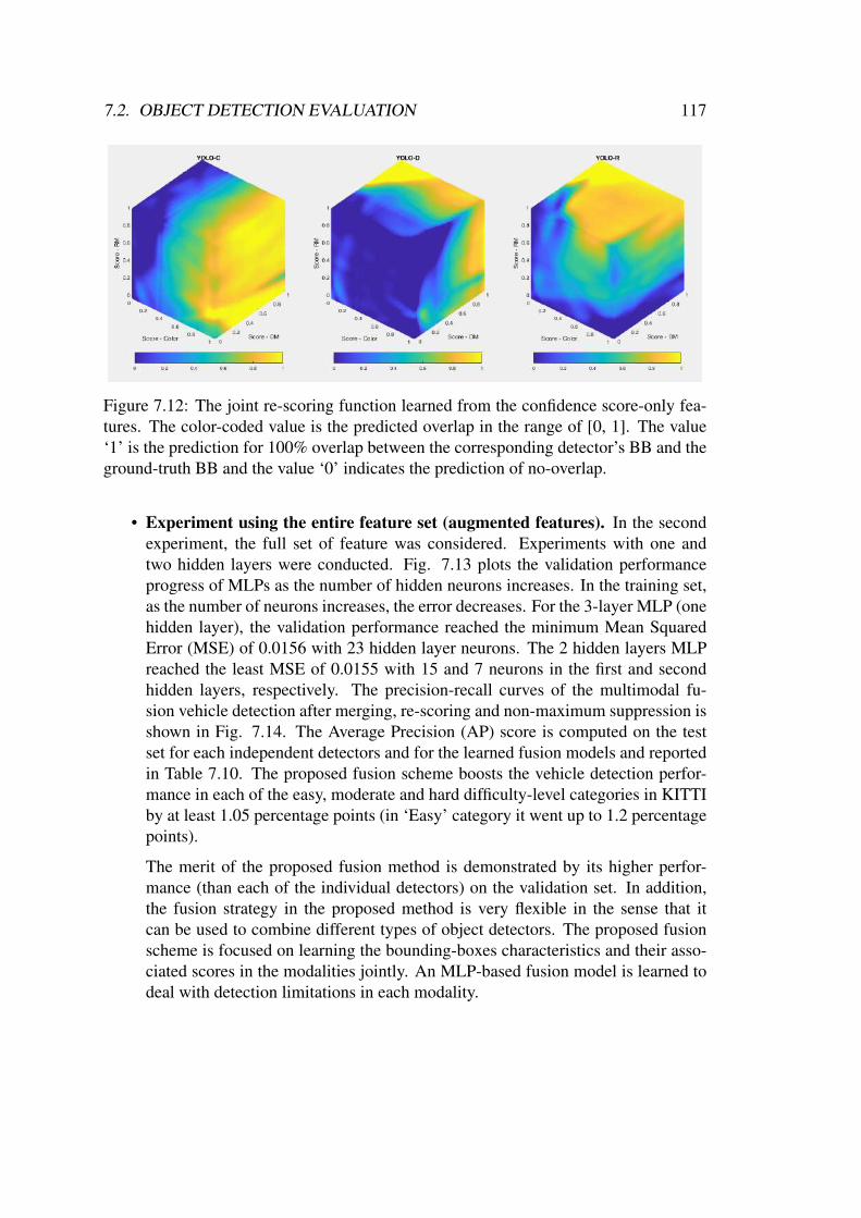
7.2. OBJECT DETECTION EVALUATION 117
Figure 7.12: The joint re-scoring function learned from the confidence score-only fea-tures. The color-coded value is the predicted overlap in the range of [0, 1]. The value‘1’ is the prediction for 100% overlap between the corresponding detector’s BB and theground-truth BB and the value ‘0’ indicates the prediction of no-overlap.
• Experiment using the entire feature set (augmented features). In the secondexperiment, the full set of feature was considered. Experiments with one andtwo hidden layers were conducted. Fig. 7.13 plots the validation performanceprogress of MLPs as the number of hidden neurons increases. In the training set,as the number of neurons increases, the error decreases. For the 3-layer MLP (onehidden layer), the validation performance reached the minimum Mean SquaredError (MSE) of 0.0156 with 23 hidden layer neurons. The 2 hidden layers MLPreached the least MSE of 0.0155 with 15 and 7 neurons in the first and secondhidden layers, respectively. The precision-recall curves of the multimodal fu-sion vehicle detection after merging, re-scoring and non-maximum suppression isshown in Fig. 7.14. The Average Precision (AP) score is computed on the testset for each independent detectors and for the learned fusion models and reportedin Table 7.10. The proposed fusion scheme boosts the vehicle detection perfor-mance in each of the easy, moderate and hard difficulty-level categories in KITTIby at least 1.05 percentage points (in ‘Easy’ category it went up to 1.2 percentagepoints).
The merit of the proposed fusion method is demonstrated by its higher perfor-mance (than each of the individual detectors) on the validation set. In addition,the fusion strategy in the proposed method is very flexible in the sense that itcan be used to combine different types of object detectors. The proposed fusionscheme is focused on learning the bounding-boxes characteristics and their asso-ciated scores in the modalities jointly. An MLP-based fusion model is learned todeal with detection limitations in each modality.

118 CHAPTER 7. EXPERIMENTAL RESULTS AND DISCUSSION
(a)
0 10 20 30 40 50
Number of hidden neurons
0.014
0.016
0.018
0.02
0.022
0.024
0.026
0.028
0.03
0.032
Mean S
quare
d E
rror
(MS
E)
1-Hidden Layer Fusion Network Performance
Train
Validation
(b)
0.0145
0.015
3
0.0155
5
0.016
0.0165
7
Mean S
quare
d E
rror
(MS
E)
0.017
9 3
0.0175
2-Hidden Layers Fusion Network Performance on the Training Set
511
# neurons in 2nd hid. layer
0.018
713 9
# neurons in 1st hid. layer
1115 1317 1519 1719
(c)
0.0155
0.016
35
0.0165
7
Mean S
quare
d E
rror
(MS
E)
0.017
9 3
2-Hidden Layers Fusion Network Performance on the Validation Set
511
# neurons in 2nd hid. layer
0.0175
713 9
# neurons in 1st hid. layer
1115 1317 1519 1719
Figure 7.13: Influence of the number of layers / hidden neurons on MLP performance.(a) shows the training and validation performances of the 3-layer MLP (i.e.1 hiddenlayer) as the number of hidden neurons increases; (b) and (c) figures show the 2 hiddenlayers MLP performance on the training and validation sets, respectively.

7.2. OBJECT DETECTION EVALUATION 119
0 0.2 0.4 0.6 0.8 1
Recall
0
0.1
0.2
0.3
0.4
0.5
0.6
0.7
0.8
0.9
1
Pre
cis
ion
AP: 75.13 62.74 53.60
Easy
Moderate
Hard
Figure 7.14: Multimodal fusion vehicle detection performance. The merged detectionsbefore (dotted-line) and after re-scoring (dashed-line), and the vehicle detection perfor-mance after re-scoring and non-maximum suppression (solid-line).
Table 7.10: Performance evaluation of the studied vehicle detectors on the KITTIDataset. YOLOv2-Color, YOLOv2-Depth, YOLOv2-Reflectance modalities and thelate fusion detection strategy are compared (‘Fusion−’ denotes the result using only theconfidence score feature subset). The figures denote Average Precision (AP) measuredat different difficulty levels. The best results are printed in bold.
Modality Easy Moderate HardColor 73.93 % 61.69 % 54.00 %Depth 68.19 % 54.59 % 47.61 %Re f lec. 68.36 % 52.23 % 45.22 %Fusion− 74.21 % 62.18 % 54.06 %Fusion 75.13 % 62.74 % 55.10 %
Evaluation on KITTI Online Benchmark
To compare with the state-of-the-art, the proposed method was evaluated on the KITTIonline object detection benchmark against methods that that also consider LIDAR data.Results are reported in Table 7.11 and Fig. 7.15. As can be noted from the table, the pro-posed method surpasses some of the approaches in the KITTI while having the shortestrunning time. In the current version of the proposed fusion detection, the input size isset as default 416 × 416 pixels. The proposed method can achieve higher detection rateby increasing the input image size at the price of slightly higher computational cost.

120 CHAPTER 7. EXPERIMENTAL RESULTS AND DISCUSSION
Table 7.11: Fusion Detection Performance on KITTI Online Benchmark.
Approach Easy Moderate Hard Run TimeMV3D [113] 90.53 % 89.17 % 80.16 % 0.363D FCN [108] 85.54 % 75.83 % 68.30 % 5MV-RGBD-RF [111] 76.49 % 69.92 % 57.47 % 4VeloFCN [107] 70.68 % 53.45 % 46.90 % 1Proposed Method 64.77 % 46.77 % 39.38 % 0.063Vote3D [106] 56.66 % 48.05 % 42.64 % 0.5CSoR [136] 35.24 % 26.13 % 22.69 % 3.5mBoW [105] 37.63 % 23.76 % 18.44 % 10
0
0.2
0.4
0.6
0.8
1
0 0.2 0.4 0.6 0.8 1
Pre
cisi
on
Recall
Car
EasyModerate
Hard
Figure 7.15: Precision-Recall on KITTI Online Benchmark (Car Class).
Computational Analysis
The proposed fusion detection method is based on a single-shot object detector (YOLOv2)which eliminates the object proposal generation step. The adopted YOLOv2, the effi-cient design and implementation of the DM, RM, and the fusion architecture of theproposed method gives high performance yet cost-effective and capable of work in real-time. The implementation environment and the computational load of the different stepsof the proposed algorithm are reported in Fig. 7.17. The modality generation and featureextraction steps are implemented in C++, YOLOv2-C/D/R are in C, and re-scoring andNMS are implemented in MATLAB (MEX enabled), respectively. The average timefor processing each frame is 63 milliseconds (about 16 frames per second). Consider-ing the synchronized camera and Velodyne LIDAR are working about 10 Hz, real-timeprocessing can be achieved by the proposed architecture.

7.2. OBJECT DETECTION EVALUATION 121
0.280.62
0.84 0.830.590.52 0.36
0.84 0.830.61
0.79
0.55
0.79
0.390.670.83
0.60.050.89
0.02
0.58 0.43
0.63 0.55
0.86
0.29 0.47 0.590.27 0.27 0.58 0.42
0.86
0.28 0.33 0.320.72
0.89
0.62
0.61
0.87
0.05 0.640.05 0.33
0.290.73
0.76 0.250.36 0.25
0.68
0.530.68
0.77 0.120.04 0.05
0.02
0.730.46 0.7 0.57 0.24 0.36 0.36
0.720.56 0.4 0.5 0.44
0.26 0.38 0.3
0.540.58 0.42 0.27
0.38 0.32 0.750.73 0.61 0.08 0.36 0.37
0.56 0.42 0.050.27 0.39 0.02
0.56 0.49 0.230.38 0.03
0.56
0.250.750.55 0.28 0.75
0.640.83
0.41
0.07 0.05 0.05 0.84
0.77 0.56 0.43 0.650.420.410.49
0.620.73 0.280.48
0.34 0.65 0.77 0.65 0.42 0.70.09 0.36 0.71
0.390.57 0.270.57 0.11
0.6 0.12
0.59 0.840.43 0.67
0.30.42 0.51 0.8 0.63 0.83
0.040.06 0.6
Figure 7.16: Fusion detection system results. Left column shows the detection resultsfrom YOLOv2-C (red), YOLOv2-D (green) and YOLOv2-R (blue) with associated con-fidence scores. Right column shows the fusion vehicle detection results (cyan) afterre-scoring and NMS compared to ground-truth (dashed-magenta).

122 CHAPTER 7. EXPERIMENTAL RESULTS AND DISCUSSION
34 ms 15 ms 2 ms 11 ms 1 ms
DM Gen.
RM Gen.
YOLO-D
YOLO-R
YOLO-C
Feature
ExtractionMLP
RescoringNMS
C++
C
MATLAB
Figure 7.17: The proposed parallel processing architecture for real-time implementa-tion, the processing time (in milliseconds), and the implementation environment of thedifferent steps of the proposed detection system.
Qualitative Results
Fig. 7.16 shows some of the most representative qualitative results using the entirefeature set. As it can be seen for most of the cases the proposed multimodal vehiclefusion system cleverly combines detection confidences of YOLOv2-C, YOLOv2-D andYOLOv2-R and outperforms each individual one.

Part III
CONCLUSIONS
123


Chapter 8
Concluding Remarks and FutureDirections
Contents8.1 Summary of Thesis Contributions . . . . . . . . . . . . . . . . . . 125
8.1.1 Obstacle Detection . . . . . . . . . . . . . . . . . . . . . . . 125
8.1.2 Object Detection . . . . . . . . . . . . . . . . . . . . . . . . 126
8.2 Discussions and Future Perspectives . . . . . . . . . . . . . . . . . 127
Every new beginning comes from someother beginning’s end.
Seneca
8.1 Summary of Thesis ContributionsThis thesis has developed multisensor object detection algorithms for autonomous driv-ing considering two different paradigms: model free (generic or class-agnostic) objectdetection based on motion cues and supervised learning based (class-specific) objectdetection.
8.1.1 Obstacle DetectionThe term ‘obstacle’ was used to refer to generic objects that stands on the ground. Theproposed obstacle detection approach (as described in Chapter 5) takes as input se-quential color images, 3D-PCDs, and the ego-vehicle’s localization data. The method
125

126 CHAPTER 8. CONCLUDING REMARKS AND FUTURE DIRECTIONS
consists on segmenting obstacles into stationary and moving parts, DATMO, and anapproach, based on the fusion of 3D-PCDs and color images, for tracking individualmoving objects.
• Static and moving obstacle detection. This section introduced the proposed4D obstacle detection algorithm (utilizing both 3D-spatial and temporal data) andwas divided into two parts: ground surface modeling using a piecewise RANSACplane fitting, and a voxel-based representation of obstacles above the estimatedground. The voxel-grid model of the environment was further segmented intostatic and moving obstacles using discriminative analysis and ego-motion infor-mation. The key contributions of this section were a novel ground surface esti-mation algorithm (which is able to model arbitrary-curve ground profiles) and asimple yet efficient method for segmenting static and moving parts of the envi-ronment.
• Motion grid-based DATMO. In previous section, we introduced a voxel repre-sentation based approach to segment moving obstacles. In this section, DATMOwas addressed in a motion grid basis. The motion grids are build using a short-term static model of the scene (using Elevation grids), followed by a properly-designed subtraction mechanism to compute the motion, and to rectify the local-ization error of the GPS-aided INS positioning system. For the object-level repre-sentation (i.e., generic moving object extraction from motion grids) a morphology-based clustering was used. The detected generic moving objects were tracked overtime using KFs with Gating and Nearest Neighbor association strategies.
• Multisensor fusion at tracking-level. As part of the overall proposed obstacledetection pipeline, we presented a multisensor 3D single-object tracking methodto improve the tracking function of the DATMO system (i.e., the proposed fu-sion tracking can be used instead of using a simple KF). In the proposed fusiontracking method, two parallel mean-shift algorithms were run individually for ob-ject localization in the color image and 3D-PCD, followed by a 2D/3D KF basedfusion and tracking. The proposed approach analyzes a sequential 2D-RGB im-age, 3D-PCD, and the ego-vehicle’s positioning data and outputs the object’s tra-jectory, current velocity estimate, and its predicted pose in the world coordinatesystem in the next time-step.
8.1.2 Object DetectionIn Chapter 6 we described the proposed methods for (class-specific) supervised learn-ing based object detection. The dataset for class-specific object detection evaluation iscomposed of a set of random images (and other sensors’ data), and the task is to detectand localize objects based on processing a single instance (frame) of sensors’ data.

8.2. DISCUSSIONS AND FUTURE PERSPECTIVES 127
• 3D-LIDAR-based object detection. In this section, an unsupervised learningtechnique is used to support (class-specific) supervised learning based object de-tection. A vehicle detection system based on the (unsupervised) hypothesis gen-eration and (supervised) hypothesis verification using 3D-LIDAR data, DBSCANclustering and a ConvNet was proposed. Specifically, hypothesis generation wasperformed by applying DBSCAN clustering on PCD data to discover structuresfrom data and to form a set of hypotheses. The produced hypotheses (nearly)correspond to distinctive obstacles over the ground, and in practice, can be usedfor free space computation to avoid collisions. Hypothesis verification was per-formed using a ConvNet applied on the generated hypotheses (in the form of adepth map).
• Multimodal object detection. This section was an extension of the previousone, and presented a multimodal fusion approach that benefits from three modal-ities, front-view dense-depth and dense-reflection maps (generated from sparse3D-LIDAR data) and a color image, for object detection. The proposed methodis composed by deep ConvNets and a Multi-Layer Perceptron (MLP) neural net-work. Deep ConvNets were run individually on the three modalities to achievedetections in the modalities. The proposed method extracts a rich set of features(e.g., detection confidence, width, height, center and so forth) from the detectionsin each modality. The desired target output of the fusion approach is defined as theoverlaps of detected bounding boxes in each modality with the ground-truth. TheMLP was trained to learn and model the nonlinear relationships among modali-ties, and to deal with the detection limitations in each modality.
8.2 Discussions and Future PerspectivesThe present study extends our knowledge of multisensor motion- and supervised learning-based object detection. The main limitations that need to be considered and some rec-ommendations for future research are presented in the following paragraphs.
• Computation time. The major part of the algorithms was implemented in MAT-LAB for rapid prototyping. Some parts were implemented in C/C++. The multi-modal fusion detection (mostly in C/C++) works at 16 fps (i.e., real-time process-ing, considering the proposed processing architecture). The proposed stationary– moving obstacle detection and multisensor single-object tracking algorithms(written mostly in MATLAB) run at about 0.3 fps and 4 fps, respectively. Thesealgorithms can be expected to achieve real-time processing after implementationin a more efficient programming language (e.g., C/C++) and exploiting pipelineparallelism.

128 CHAPTER 8. CONCLUDING REMARKS AND FUTURE DIRECTIONS
• Sensor fusion. We studied sensor/modality fusion for object detection and track-ing tasks. A low-level and high-level (KF-based) multisensor fusion methods forobject tracking were developed and analyzed in this thesis. The low-level fu-sion, denoted by ‘L-Fus.’, was presented in Chapter 7 as a comparative methodfor assessing the proposed ‘H-Fus.’ fusion tracking approach. We showed thatthe high-level fusion offers higher performance than the low-level method in theproposed tracking pipeline. For the purpose of multisensor multimodal objectdetection, a high-level (learning-based) multimodal fusion, based on two sensors(color camera and 3D-LIDAR) in three modalities (color image, 3D-LIDAR’srange and reflectance data), was studied in this thesis. The proposed fusion de-tection method, besides being able to work in real-time (considering the proposedparallel processing architecture), learns the nonlinear relationships among modal-ities and deals with the detection limitations of each modality. Incorporating mul-tiple level of data abstraction in the fusion framework can be explored as futurework (e.g., integrating multiple feature-map layers of a ConvNet-based object de-tection into the fusion framework to obtain a more accurate object detection).
• Multi-view detection. In Chapter 6, the supervised learning based object de-tection was described. Specifically, in the second part of Chapter 6, front-viewdense multimodal maps from 3D-LIDAR (i.e., range and reflectance maps) wereexplored for class-specific object detection. We suggest that in future researchthe incorporation of other 3D-LIDAR views (e.g., top view in the form of an Ele-vation grid representation) in the fusion framework for object detection could beresearched.
• Integrating temporal data to improve the object detection performance. Oneof the less researched issues in the state-of-the-art is how much temporal data(e.g., in the form of moving object detection) can improve per-frame detectionresults. We anticipate that integrating temporal data into the object detection pro-cess would increase its performance. Taking into account this thesis’ findings (onmotion- and supervised learning-based object detection), we suggest that futureresearch should look into exploiting temporal data to enhance the performance ofthe class-specific object detection.
• Benchmarking. The lack of annotated datasets for obstacle (or generic object)detection evaluation was one of the main challenges for developing this thesis. Weintroduced some benchmarks (extracted out of the KITTI dataset) for the evalua-tion of ground surface estimation (in three dimensions), stationary – moving ob-stacle detection and 3D single-object tracking performances. Obstacle detectionbenchmarking, although very challenging, could be a future direction to acceler-ate the research toward real-world autonomous driving.

Appendices
129


Appendix A
3D Multisensor Single-Object TrackingBenchmark
131

132APPENDIX A. 3D MULTISENSOR SINGLE-OBJECT TRACKING BENCHMARK
Previous attempts to propose object tracking benchmarks for automotive applica-tions were mostly based on monocular cameras [73, 74], or were just focused on thedata association problem [137]. A benchmark dataset, called 3D Object Tracking inDriving Environment (3D-OTD), is proposed (based on the ‘KITTI Object TrackingEvaluation’) to facilitate the evaluation of appearance modeling in single-object track-ing using a multimodal perception system of autonomous vehicles. Therefore, instead oftracklets, full track of each object is extracted. A benchmark dataset with 50 annotatedsequences is constructed out of the ‘KITTI Object Tracking Evaluation’ to facilitate theperformance evaluation. In the constructed benchmark dataset, each sequence denotesa trajectory of only one target object (i.e., if one scenario includes two target objects, itis considered as two sequences).
The specifications of each sequence and the most challenging factors are extractedand reported in Table A.1. The table contains the description of the scene, sequence,and objects including the number of frames for each sequence, object type: car ‘C’,pedestrian ‘P’ and cyclist ‘Y’, object and Ego-vehicle situations: moving ‘M’ or sta-tionary ‘S’, scene condition: roads in urban environment ‘U’ or alleys in downtown‘D’. The object width (Im-W) and height (Im-H) in the first frame (in pixels), and width(PCD-W), height (PCD-H), and length (PCD-L) in the first PCD (in meters) of eachsequence are also reported. Each of the sequences are categorized according to the fol-lowing challenges: occlusion (OCC), object pose (POS) and distance (DIS) variations toEgo-vehicle, and changes in the relative velocity (RVL) of the object to the Ego-vehicle.
A.1 Baseline 3D Object Tracking AlgorithmsAs a starting point for the benchmark, two generative 3D-LIDAR-based methods wereimplemented as baselines for evaluation purposes. The baseline methods take LIDARPCDs as the input (after a ground removal process). The initial position of the Object’s3D Bounding Box (3D-OBB) is known, the size of the 3D-BB is assumed fixed duringthe tracking, and the ‘point model’ is used for the object representation.
• Baseline KF 3D Object Tracker (3D-KF). A 3D Constant Acceleration (CA) KFwith a Gating Data Association (DA) is used for the robust tracking of the objectcentroid in the consecutive PCDs. The state of the filter is x=
[x, x, x,y, y, y,z, z, z
]>,where x, y, z and x, y, z are velocity and acceleration in x,y,z location, respectively.To eliminate outliers and increase the robustness of the process, the search areais limited to a gate in the vicinity of the predicted KF location from the previ-ous step. If no measurement is available inside the gate area, the predicted KFvalue is used. Experiments with different gate sizes (1×3D-OBB, 1.5×3D-OBBand 2× 3D-OBB) were performed to conclude that the gate size of 1× 3D-OBBprovides a better result.

A.1. BASELINE 3D OBJECT TRACKING ALGORITHMS 133
Table A.1: Detailed information and challenging factors for each sequence.
ID #Frm. Obj. Obj.
StatusEgo.
StatusSceneCond. Im-W Im-H PCD-H PCD-W PCD-L OCC POS DIS RVL
1 154 C M M U 178 208 1.73 0.82 1.78 * * *2 154 Y M M U 154 127 2.00 1.82 4.43 * *3 101 C S M U 93 42 2.19 1.89 5.53 * *4 18 C S M U 77 52 1.52 1.55 3.57 *5 58 C S M U 19 17 1.54 1.66 4.14 *6 144 P S M U 16 42 1.72 0.73 0.55 *7 78 C M M U 54 21 1.48 1.59 3.46 * * *8 78 C M M U 193 77 3.01 2.59 11.84 * *9 122 C M M U 100 302 1.59 1.65 3.55 *10 314 C M M U 152 87 1.64 1.67 3.63 * * *11 297 C M M U 36 36 1.62 1.62 4.50 *12 101 Y M M U 8 26 1.64 0.33 1.57 *13 42 Y M M U 15 36 1.64 0.33 1.57 * *14 136 C M M U 95 34 1.47 1.35 3.51 * * * *15 38 C S M U 98 34 1.45 1.63 4.20 *16 51 C M M U 52 34 1.57 1.65 4.10 * *17 42 C M M U 22 19 1.85 1.67 4.09 *18 31 C S M U 52 34 1.45 1.60 4.22 *19 24 C M M U 30 32 3.43 2.81 7.02 *20 390 C M M U 18 13 1.25 1.59 3.55 *21 36 C S M U 28 32 2.71 1.89 5.77 *22 65 C S M U 76 28 1.72 1.73 4.71 *23 56 C M M U 152 57 3.52 2.89 10.81 * * *24 474 C M M U 274 97 3.52 2.89 10.81 * * * *25 63 P M M U 16 30 1.63 0.40 0.83 *26 99 Y M M D 39 39 1.81 0.59 1.89 * * *27 41 P M M D 25 42 1.53 0.61 0.73 *28 323 Y S M U 25 38 1.72 0.78 1.70 *29 188 C M M U 30 21 1.44 1.74 4.23 * * *30 51 C M M U 126 37 1.50 1.54 4.09 * * * *31 41 P M S D 70 105 1.63 0.66 0.89 *32 131 P M S D 46 65 1.76 0.90 1.11 * * *33 132 P M S D 43 72 1.89 0.84 1.05 * *34 140 P M S D 33 63 1.83 0.73 1.16 * *35 141 P M S D 27 58 1.70 0.65 1.10 * *36 112 P M S D 33 66 1.84 0.78 1.03 * *37 31 Y M S D 35 47 1.84 0.50 1.60 * *38 112 P M S D 20 54 1.67 0.44 0.75 * *39 145 P M S D 19 53 1.95 0.62 0.74 * *40 54 P M S D 101 160 1.71 0.48 0.93 *41 45 P M S D 196 224 1.64 0.55 0.94 *42 264 C M M U 28 24 1.40 1.54 3.36 * *43 71 P M M D 89 124 1.61 0.91 0.91 *44 125 P M M D 36 62 1.64 0.88 0.49 * *45 146 V S M D 45 56 2.56 2.05 5.86 *46 156 P M M D 25 48 1.88 0.95 0.94 *47 45 P M M D 29 58 1.67 0.70 0.94 * *48 188 P M M D 31 67 1.76 0.76 1.01 * *49 359 P M M D 28 51 1.80 0.90 0.94 * *50 360 P M M D 26 49 1.72 0.84 0.85 * *
• Baseline MS 3D Object Tracker (3D-MS). In the 3D-MS approach, the MeanShift (MS) iterative procedure is used to locate the object, as follows:

134APPENDIX A. 3D MULTISENSOR SINGLE-OBJECT TRACKING BENCHMARK
1. The shift-vector between the center of 3D-BB and centroid of point set Pinside the 3D-BB is computed.
2. The 3D-BB is translated using the shift-vector.
3. Iterate steps 1 and 2 until convergence: The MS iteratively shifts the 3D-BBuntil the object is placed entirely within the 3D-BB. MS is considered con-verged when the centroid movement |mk| < 0.5m or the maximum numberof iterations is met.
We conducted an experiment with different maximum number of iterations (3, 5and 10) and observed that a maximum of 3 iterations provides a better result. Theobject orientation is achieved by subtracting the current estimated location andthe previous location of the object.
A.2 Quantitative Evaluation MethodologyDifferent metrics have been proposed for the evaluation of object tracking methods [138,139, 140]. For the quantitative evaluation, two assessment criteria are used as follows:
• The precision plot of overlap success. The overlap rate (the intersection-over-union metric) in 3D is given by
O3D =volume(3D-BB∩3D-BBG)
volume(3D-BB∪3D-BBG)(A.1)
where 3D-BBG is the Ground-Truth (GT) 3D-BBs available in the KITTI dataset.The overlap rate ranges from 0 to 1. To be correct (to be considered a success), theoverlap ratio O3D must exceed 0.25, which is a standard threshold. The percentageof frames with a successful occurrence is used as a metric to measure trackingperformance.
• The precision plot of orientation success. The GT for the orientation of theobject in the KITTI dataset is given by the Yaw angle (Yaw angle describes theheading of the object, and corresponds to the rotation around z-axis) The orienta-tion error can be computed by
Eθ = |−→θ −
−→θ
G| (A.2)
where−→θ G is the GT orientation of the object. The precision plot of orientation is
given by the percentage of frames with Eθ less than a certain threshold (this valueis empirically set as 10 degrees).

A.3. EVALUATION RESULTS AND ANALYSIS OF METRICS 135
0 0.1 0.2 0.3 0.4 0.5 0.6 0.7 0.8 0.9 1
0
0.1
0.2
0.3
0.4
0.5
0.6
0.7
0.8
0.9
13D-BB Overlap - OCC
3D-KF
3D-MS
0 0.1 0.2 0.3 0.4 0.5 0.6 0.7 0.8 0.9 1
0
0.1
0.2
0.3
0.4
0.5
0.6
0.7
0.8
0.9
13D-BB Overlap - POS
3D-KF
3D-MS
0 0.1 0.2 0.3 0.4 0.5 0.6 0.7 0.8 0.9 1
0
0.1
0.2
0.3
0.4
0.5
0.6
0.7
0.8
0.9
13D-BB Overlap - DIS
3D-KF
3D-MS
0 0.1 0.2 0.3 0.4 0.5 0.6 0.7 0.8 0.9 1
0
0.1
0.2
0.3
0.4
0.5
0.6
0.7
0.8
0.9
13D-BB Overlap - RVL
3D-KF
3D-MS
Figure A.1: The precision plot of 3D overlap rate based on OCC, POS, DIS and RVLchallenges.
A.3 Evaluation Results and Analysis of MetricsThe metrics for the two baseline trackers (3D-MS and 3D-KF) are computed based onOCC, POS, DIS and RVL challenges and plotted in Fig. A.1 and Fig. A.2, where x-axis denotes normalized number of the frames in all the sequences and y-axis showsnormalized cumulative sum of the successful cases (i.e. each frame in which the 3DBB overlap or orientation error condition is met gets added to the cumulative sum). The3D-KF achieves higher success rate because the 3D-MS tracker may diverge to a densernearby object (a local minima) instead of tracking the target object. Interestingly, 3D-KF performs much better in the RVL challenge because of a more accurate estimationof the object dynamics. However, the 3D-MS tracker has a higher precision in theorientation estimation. The average computation time of baseline trackers is about 15fps. The experiment was carried out using a quad core 3.4 GHz processor with 8 GB

136APPENDIX A. 3D MULTISENSOR SINGLE-OBJECT TRACKING BENCHMARK
0 0.1 0.2 0.3 0.4 0.5 0.6 0.7 0.8 0.9 1
0
0.1
0.2
0.3
0.4
0.5
0.6
0.7
0.8
0.9
1Pose - OCC
3D-KF
3D-MS
0 0.1 0.2 0.3 0.4 0.5 0.6 0.7 0.8 0.9 1
0
0.1
0.2
0.3
0.4
0.5
0.6
0.7
0.8
0.9
1Pose - POS
3D-KF
3D-MS
0 0.1 0.2 0.3 0.4 0.5 0.6 0.7 0.8 0.9 1
0
0.1
0.2
0.3
0.4
0.5
0.6
0.7
0.8
0.9
1Pose - DIS
3D-KF
3D-MS
0 0.1 0.2 0.3 0.4 0.5 0.6 0.7 0.8 0.9 1
0
0.1
0.2
0.3
0.4
0.5
0.6
0.7
0.8
0.9
1Pose - RVL
3D-KF
3D-MS
Figure A.2: The precision plot of orientation error based on OCC, POS, DIS and RVLchallenges.
RAM under MATLAB R2015a.
A.3.1 A Comparison of Baseline Trackers with the State-of-the-artComputer Vision based Object Trackers
3D-LIDAR sensors are opening their way for high-level perception tasks in computervision, like object tracking, object recognition, and scene understanding. We found itinteresting to compare our baseline trackers (3D-MS and 3D-KF) with two high-rankingstate-of-the-art computer vision based object trackers (SCM [141], and ASLA [142]) inthe Object Tracking Benchmark [138]. SCM and ASLA run at about 1 fps and 6.5 fps,respectively. The precision plot is given by the percentage of successful occurrences(localization error less than 20 pixels [138]), and is presented in Fig. A.3.

A.3. EVALUATION RESULTS AND ANALYSIS OF METRICS 137
0 0.1 0.2 0.3 0.4 0.5 0.6 0.7 0.8 0.9 1
0
0.1
0.2
0.3
0.4
0.5
0.6
0.7
0.8
0.9
1Precision Plot - LOC
3D-KF
3D-MS
SCM
ASLA
Figure A.3: The precision plot of location error.
We found that our baseline trackers, benefiting from highly reliable 3D-LIDARdata, have superior performance over the state-of-the-art approaches in Computer Vi-sion field. This is because, in autonomous driving scenarios, ego-vehicle and objectsare often moving. Therefore, object size and pose undergo severe changes (in the RGBimage), which can easily mislead visual object trackers.

138APPENDIX A. 3D MULTISENSOR SINGLE-OBJECT TRACKING BENCHMARK

Appendix B
Object Detection Using Reflection Data
139

140 APPENDIX B. OBJECT DETECTION USING REFLECTION DATA
Table B.1: The RefCN processing time (in milliseconds).
Impl. Details Proc. Time EnvironmentRM Generation 34 C++YOLOv2 Detection 15 C
In this appendix, an object detection method using 3D-LIDAR reflection intensitydata and YOLOv2 416×416 object detection framework is presented (herein called Re-fCN, which stands for ‘Reflectance ConvNet’). The front-view dense Reflection Map(RM) runs through the trained RM-based YOLOv2 pipeline to achieve object detec-tion. For this analysis, the KITTI object detection ‘training dataset’ (containing 7481frames) was partitioned into two subsets: 80 % as training set (5985 frames) and 20 %as validation set (1496 frames). The ‘Car’ label was considered for the evaluation.
B.1 Computational Complexity and Run-TimeThe experiments were run on a computer with a Hexa-core 3.5 GHz processor, poweredwith a GTX 1080 GPU and 64 GB RAM under Linux. Two versions of RM were im-plemented: a version using MATLAB scatteredInterpolant function and a much fasterreimplementation in C++. The RM generation in MATLAB takes about 1.4 secondswhile in C++ it takes 34 ms. The implementation details and the computational loadof RM generation and YOLOv2 detection steps are reported in Table B.1. The over-all time for processing each frame using C++ implementation is 49 milliseconds (morethan 20 frames per second). Considering that the KITTI dataset was captured using a10 Hz spinning Velodyne HDL-64E, it can be concluded that RefCN can be performedin real-time.
B.2 Quantitative ResultsQuantitative experiments were conducted to assess the performance of the RefCN: (i)Sparse Reflectance Map versus RM; (ii) comparison of RMs with different interpolationmethods; (iii) RM versus color and range data modalities; and (iv) RefCN versus state-of-the-art methods.
B.2.1 Sparse Reflectance Map vs RMThe RefCN was trained on training set and evaluated on the validation set. As can beseen from Fig. B.1 and Table B.2, the results show that the RM (with the default inputsize of 416×416 and the Nearest Neighbor interpolation) considerably improves the

B.2. QUANTITATIVE RESULTS 141
0 0.1 0.2 0.3 0.4 0.5 0.6 0.7 0.8 0.9 1Recall
0
0.1
0.2
0.3
0.4
0.5
0.6
0.7
0.8
0.9
1
Pre
cisi
onEasyModerateHard
Figure B.1: Precision-Recall using sparse RM (dashed lines) versus RM (solid lines) onKITTI validation-set (Car class).
Table B.2: Detection accuracy with sparse RM vs RM on validation-set.
Input Data Easy Moderate HardSparse RM 23.45 % 17.57 % 15.57 %RM 67.69 % 51.91 % 44.98 %RM* 72.67 % 62.65 % 54.89 %
detection performance in comparison with the sparse Reflectance Map. In Table B.2,RM* denotes the results for an increased input size of 1216×352. For the rest of thisdocument, the analyses were performed for the default input size of 416×416.
B.2.2 RM Generation Using Nearest Neighbor, Linear and NaturalInterpolations
The result from the previous experiment shows that the use of dense up-sampled rep-resentation considerably improves the detection rate. A question that can be raised iswhich interpolation method gives the best performance. In this experiment, we eval-uated three interpolation methods: Nearest Neighbor (RMnearest), Natural Neighbor(RMnatural) and Linear (RMlinear) Interpolation. RMnatural is based on Voronoi tessel-

142 APPENDIX B. OBJECT DETECTION USING REFLECTION DATA
0 0.1 0.2 0.3 0.4 0.5 0.6 0.7 0.8 0.9 1Recall
0
0.1
0.2
0.3
0.4
0.5
0.6
0.7
0.8
0.9
1
Pre
cisi
on
EasyModerateHard
Figure B.2: Precision-Recall using RMnearest (solid lines), RMnatural (dashed lines) andRMlinear (dotted lines) on KITTI Validation-set (Car class).
Table B.3: Detection accuracy using RM with different interpolation methods onvalidation-set.
Input Data Easy Moderate HardRM (RMnearest) 67.69 % 51.91 % 44.98 %RMlinear 60.60 % 45.71 % 40.79 %RMnatural 65.25 % 50.07 % 44.76 %
lation of the projected LIDAR points which result in a continuous surface except atprojected points. RMlinear is based on linear interpolation between sets of three points(of the projected LIDAR points) for surfaces in Delaunay Triangulation (DT) format.Fig. B.3 shows an example of a color image and the corresponding generated RMs. Thedetection performance for each interpolation method is reported in Fig. B.2 and TableB.3. The best performance was attained, for all categories, with RMnearest.
B.3 Qualitative ResultsFigure B.4 shows some of the representative qualitative results with many cars in thescene. As can be seen, for most cases, the RefCN correctly detects target vehicles.

B.3. QUALITATIVE RESULTS 143
(a)
(b)
(c)
(d)
Figure B.3: Top to bottom: (a) an example of color image from KITTI dataset, (b) thegenerated RMnearest, (c) RMnatural and (d) RMlinear, respectively.
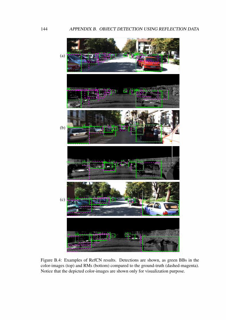
144 APPENDIX B. OBJECT DETECTION USING REFLECTION DATA
(a)0.83 0.7 0.62 0.7 0.55 0.71 0.63 0.770.81
0.87
0.83 0.7 0.62 0.7 0.55 0.71 0.63 0.770.81
0.87
(b)0.58 0.7 0.56 0.37
0.36 0.5 0.780.91 0.46
0.9
0.58 0.7 0.56 0.370.36 0.5 0.78
0.91 0.46
0.9
(c)0.78 0.7 0.68 0.39 0.490.3
0.80.93
0.78 0.7 0.68 0.39 0.490.30.8
0.93
Figure B.4: Examples of RefCN results. Detections are shown, as green BBs in thecolor-images (top) and RMs (bottom) compared to the ground-truth (dashed-magenta).Notice that the depicted color-images are shown only for visualization purpose.

Bibliography
[1] Martin Ester, Hans-Peter Kriegel, Jorg Sander, Xiaowei Xu, et al. A density-based algorithm for discovering clusters in large spatial databases with noise. InKDD, volume 96, pages 226–231, 1996.
[2] K Bhalla, M Shotten, A Cohen, M Brauer, S Shahraz, R Burnett, K Leach-Kemon, G Freedman, and CJ Murray. Transport for health: the global burdenof disease from motorized road transport. World Bank Group: Washington, DC,2014.
[3] Etienne Krug. Decade of action for road safety 2011–2020. Injury, 43(1):6–7,2012.
[4] Santokh Singh. Critical reasons for crashes investigated in the national motorvehicle crash causation survey. Technical report, Traffic Safety Facts Crash Stats,National Highway Traffic Safety Administration, Washington, DC, 2015.
[5] Chris Urmson, Joshua Anhalt, Drew Bagnell, Christopher Baker, Robert Bittner,M. N. Clark, John Dolan, Dave Duggins, Tugrul Galatali, Chris Geyer, MicheleGittleman, Sam Harbaugh, Martial Hebert, Thomas M. Howard, Sascha Kol-ski, Alonzo Kelly, Maxim Likhachev, Matt McNaughton, Nick Miller, KevinPeterson, Brian Pilnick, Raj Rajkumar, Paul Rybski, Bryan Salesky, Young-Woo Seo, Sanjiv Singh, Jarrod Snider, Anthony Stentz, William Red Whittaker,Ziv Wolkowicki, Jason Ziglar, Hong Bae, Thomas Brown, Daniel Demitrish,Bakhtiar Litkouhi, Jim Nickolaou, Varsha Sadekar, Wende Zhang, Joshua Stru-ble, Michael Taylor, Michael Darms, and Dave Ferguson. Autonomous drivingin urban environments: Boss and the urban challenge. Journal of Field Robotics,25(8):425–466, 2008.
[6] Michael Montemerlo, Jan Becker, Suhrid Bhat, Hendrik Dahlkamp, DmitriDolgov, Scott Ettinger, Dirk Haehnel, Tim Hilden, Gabe Hoffmann, BurkhardHuhnke, et al. Junior: The stanford entry in the urban challenge. Journal of fieldRobotics, 25(9):569–597, 2008.
145

146 BIBLIOGRAPHY
[7] Peter Corke. Robotics, Vision and Control: Fundamental Algorithms In MAT-LAB® Second, Completely Revised, volume 118. Springer, 2017.
[8] Paul J Besl, Neil D McKay, et al. A method for registration of 3-d shapes. IEEETransactions on pattern analysis and machine intelligence, 14(2):239–256, 1992.
[9] Jon Louis Bentley. Multidimensional binary search trees used for associativesearching. Communications of the ACM, 18(9):509–517, 1975.
[10] Hugh F Durrant-Whyte. Sensor models and multisensor integration. The inter-national journal of robotics research, 7(6):97–113, 1988.
[11] Belur V Dasarathy. Decision fusion, volume 1994. IEEE Computer Society PressLos Alamitos, CA, 1994.
[12] R Boudjemaa and AB Forbes. Parameter estimation methods for data fusion,national physical laboratory report no. CMSC 38, 4, 2004.
[13] Federico Castanedo. A review of data fusion techniques. The Scientific WorldJournal, 2013, 2013.
[14] Shai Shalev-Shwartz and Shai Ben-David. Understanding machine learning:From theory to algorithms. Cambridge university press, 2014.
[15] Ian Goodfellow, Yoshua Bengio, Aaron Courville, and Yoshua Bengio. Deeplearning, volume 1. MIT press Cambridge, 2016.
[16] Kurt Hornik, Maxwell Stinchcombe, and Halbert White. Multilayer feedforwardnetworks are universal approximators. Neural networks, 2(5):359–366, 1989.
[17] Yanming Guo, Yu Liu, Ard Oerlemans, Songyang Lao, Song Wu, and Michael SLew. Deep learning for visual understanding: A review. Neurocomputing,187:27–48, 2016.
[18] Nitish Srivastava, Geoffrey E Hinton, Alex Krizhevsky, Ilya Sutskever, and Rus-lan Salakhutdinov. Dropout: a simple way to prevent neural networks from over-fitting. Journal of machine learning research, 15(1):1929–1958, 2014.
[19] Y. LeCun, L. Bottou, Y. Bengio, and P. Haffner. Gradient-based learning appliedto document recognition. Proceedings of the IEEE, 86(11):2278–2324, 1998.
[20] A Geiger, P Lenz, C Stiller, and R Urtasun. Vision meets robotics: The KITTIdataset. The International Journal of Robotics Research, 32(11):1231–1237,2013.

BIBLIOGRAPHY 147
[21] Joel Janai, Fatma Guney, Aseem Behl, and Andreas Geiger. Computer vision forautonomous vehicles: Problems, datasets and state-of-the-art. ARXIV, 2017.
[22] Mark Everingham, Luc Van Gool, Christopher KI Williams, John Winn, and An-drew Zisserman. The pascal visual object classes (voc) challenge. Internationaljournal of computer vision, 88(2):303–338, 2010.
[23] Andreas Geiger, Philip Lenz, and Raquel Urtasun. Are we ready for autonomousdriving? the kitti vision benchmark suite. In CVPR, 2012.
[24] Joseph Redmon, Santosh Divvala, Ross Girshick, and Ali Farhadi. You only lookonce: Unified, real-time object detection. In CVPR, pages 779–788, 2016.
[25] Joseph Redmon and Ali Farhadi. Yolo9000: Better, faster, stronger. In CVPR,2017.
[26] Andreas Nuchter, Kai Lingemann, Joachim Hertzberg, and Hartmut Surmann. 6dslam with approximate data association. In Advanced Robotics, 2005. ICAR’05.Proceedings., 12th International Conference on, pages 242–249. IEEE, 2005.
[27] Daniel Sack and Wolfram Burgard. A comparison of methods for line extractionfrom range data. In Proc. of the 5th IFAC symposium on intelligent autonomousvehicles (IAV), 2004.
[28] Miguel Oliveira, Victor Santos, Angel Sappa, and P.Dias. Scene representationsfor autonomous driving: an approach based on polygonal primitives. In 2ndIberian Robotics Conference, 2015.
[29] Ricardo Pascoal, Vitor Santos, Cristiano Premebida, and Urbano Nunes. Simul-taneous segmentation and superquadrics fitting in laser-range data. VehicularTechnology, IEEE Transactions on, 64(2):441–452, 2015.
[30] Hans P Moravec and Alberto Elfes. High resolution maps from wide angle sonar.In Robotics and Automation. Proceedings. 1985 IEEE International Conferenceon, volume 2, pages 116–121. IEEE, 1985.
[31] M Herbert, C Caillas, Eric Krotkov, In So Kweon, and Takeo Kanade. Terrainmapping for a roving planetary explorer. In Robotics and Automation, 1989.Proceedings., 1989 IEEE International Conference on, pages 997–1002. IEEE,1989.
[32] Patrick Pfaff, Rudolph Triebel, and Wolfram Burgard. An efficient extension toelevation maps for outdoor terrain mapping and loop closing. The InternationalJournal of Robotics Research, 26(2):217–230, 2007.

148 BIBLIOGRAPHY
[33] Rudolph Triebel, Patrick Pfaff, and Wolfram Burgard. Multi-level surface mapsfor outdoor terrain mapping and loop closing. In Intelligent Robots and Systems,2006 IEEE/RSJ International Conference on, pages 2276–2282. IEEE, 2006.
[34] Yuval Roth-Tabak and Ramesh Jain. Building an environment model using depthinformation. Computer, 22(6):85–90, 1989.
[35] H Moravec. Robot spatial perceptionby stereoscopic vision and 3d evidencegrids. Perception,(September), 1996.
[36] D. Haehnel. Mapping with Mobile Robots. PhD thesis, University of Freiburg,Department of Computer Science, December 2004.
[37] Julian Ryde and Huosheng Hu. 3d mapping with multi-resolution occupied voxellists. Autonomous Robots, 28(2):169–185, 2010.
[38] Bertrand Douillard, J Underwood, Narek Melkumyan, S Singh, Shrihari Vasude-van, C Brunner, and A Quadros. Hybrid elevation maps: 3d surface models forsegmentation. In Intelligent Robots and Systems (IROS), 2010 IEEE/RSJ Inter-national Conference on, pages 1532–1538. IEEE, 2010.
[39] Donald Meagher. Geometric modeling using octree encoding. Computer graph-ics and image processing, 19(2):129–147, 1982.
[40] Armin Hornung, KaiM. Wurm, Maren Bennewitz, Cyrill Stachniss, and WolframBurgard. Octomap: an efficient probabilistic 3d mapping framework based onoctrees. Autonomous Robots, 34(3):189–206, 2013.
[41] Ivan Dryanovski, William Morris, and Jizhong Xiao. Multi-volume occupancygrids: An efficient probabilistic 3d mapping model for micro aerial vehicles. InIntelligent Robots and Systems (IROS), 2010 IEEE/RSJ International Conferenceon, pages 1553–1559. IEEE, 2010.
[42] Anca Discant, Alexandrina Rogozan, Calin Rusu, and Abdelaziz Bensrhair. Sen-sors for obstacle detection-a survey. In Electronics Technology, 30th Interna-tional Spring Seminar on, pages 100–105. IEEE, 2007.
[43] Nicola Bernini, Massimo Bertozzi, Luca Castangia, Marco Patander, and MarioSabbatelli. Real-time obstacle detection using stereo vision for autonomousground vehicles: A survey. In Intelligent Transportation Systems (ITSC), 2014IEEE 17th International Conference on, pages 873–878. IEEE, 2014.
[44] Anna Petrovskaya, Mathias Perrollaz, Luciano Oliveira, Luciano Spinello,Rudolph Triebel, Alexandros Makris, John-David Yoder, Christian Laugier, Ur-bano Nunes, and Pierre Bessiere. Awareness of road scene participants for
BIBLIOGRAPHY 149
autonomous driving. In Handbook of Intelligent Vehicles, pages 1383–1432.Springer, 2012.
[45] Sayanan Sivaraman and Mohan Manubhai Trivedi. Looking at vehicles on theroad: A survey of vision-based vehicle detection, tracking, and behavior analy-sis. Intelligent Transportation Systems, IEEE Transactions on, 14(4):1773–1795,2013.
[46] Zhongfei Zhang, Richard Weiss, and Allen R Hanson. Obstacle detection basedon qualitative and quantitative 3d reconstruction. Pattern Analysis and MachineIntelligence, IEEE Transactions on, 19(1):15–26, 1997.
[47] D. Pfeiffer and U. Franke. Efficient representation of traffic scenes by meansof dynamic stixels. In Intelligent Vehicles Symposium (IV), 2010 IEEE, pages217–224, June 2010.
[48] A. Broggi, S. Cattani, M. Patander, M. Sabbatelli, and P. Zani. A full-3d voxel-based dynamic obstacle detection for urban scenario using stereo vision. In In-telligent Transportation Systems - (ITSC), 2013 16th International IEEE Confer-ence on, pages 71–76, Oct 2013.
[49] A. Azim and O. Aycard. Layer-based supervised classification of moving objectsin outdoor dynamic environment using 3d laser scanner. In Intelligent VehiclesSymposium Proceedings, 2014 IEEE, pages 1408–1414, June 2014.
[50] Raphael Labayrade, Didier Aubert, and Jean-Philippe Tarel. Real time obstacledetection in stereovision on non flat road geometry through” v-disparity” repre-sentation. In Intelligent Vehicle Symposium, 2002. IEEE, volume 2, pages 646–651. IEEE, 2002.
[51] Angel D Sappa, Rosa Herrero, Fadi Dornaika, David Geronimo, and AntonioLopez. Road approximation in euclidean and v-disparity space: a comparativestudy. In Computer Aided Systems Theory–EUROCAST 2007, pages 1105–1112.Springer, 2007.
[52] Florin Oniga and Sergiu Nedevschi. Processing dense stereo data using elevationmaps: Road surface, traffic isle, and obstacle detection. Vehicular Technology,IEEE Transactions on, 59(3):1172–1182, 2010.
[53] Martin A Fischler and Robert C Bolles. Random sample consensus: a paradigmfor model fitting with applications to image analysis and automated cartography.Communications of the ACM, 24(6):381–395, 1981.

150 BIBLIOGRAPHY
[54] Anna V Petrovskaya. Towards dependable robotic perception. Stanford Univer-sity, 2011.
[55] John Leonard, Jonathan How, Seth Teller, Mitch Berger, Stefan Campbell, Gas-ton Fiore, Luke Fletcher, Emilio Frazzoli, Albert Huang, Sertac Karaman, et al.A perception-driven autonomous urban vehicle. Journal of Field Robotics,25(10):727–774, 2008.
[56] Jaebum Choi, Simon Ulbrich, Bernd Lichte, and Markus Maurer. Multi-targettracking using a 3d-lidar sensor for autonomous vehicles. In 16th InternationalIEEE Conference on Intelligent Transportation Systems (ITSC 2013), pages 881–886. IEEE, 2013.
[57] Christoph Mertz, Luis E Navarro-Serment, Robert MacLachlan, Paul Rybski,Aaron Steinfeld, Arne Suppe, Christopher Urmson, Nicolas Vandapel, MartialHebert, Chuck Thorpe, et al. Moving object detection with laser scanners. Jour-nal of Field Robotics, 30(1):17–43, 2013.
[58] Andreas Ess, Konrad Schindler, Bastian Leibe, and Luc Van Gool. Object de-tection and tracking for autonomous navigation in dynamic environments. TheInternational Journal of Robotics Research, 29(14):1707–1725, 2010.
[59] Siavash Hosseinyalamdary, Yashar Balazadegan, and Charles Toth. Tracking 3dmoving objects based on gps/imu navigation solution, laser scanner point cloudand gis data. ISPRS International Journal of Geo-Information, 4(3):1301–1316,2015.
[60] Anna Petrovskaya and Sebastian Thrun. Model based vehicle detection and track-ing for autonomous urban driving. Autonomous Robots, 26(2-3):123–139, 2009.
[61] Takeo Miyasaka, Yoshihiro Ohama, and Yoshiki Ninomiya. Ego-motion estima-tion and moving object tracking using multi-layer lidar. In Intelligent VehiclesSymposium, 2009 IEEE, pages 151–156. IEEE, 2009.
[62] Josip Cesic, Ivan Markovic, Srecko Juric-Kavelj, and Ivan Petrovic. Short-termmap based detection and tracking of moving objects with 3d laser on a vehicle.In Informatics in Control, Automation and Robotics, pages 205–222. Springer,2016.
[63] Andrei Vatavu, Radu Danescu, and Sergiu Nedevschi. Stereovision-based mul-tiple object tracking in traffic scenarios using free-form obstacle delimitersand particle filters. Intelligent Transportation Systems, IEEE Transactions on,16(1):498–511, 2015.

BIBLIOGRAPHY 151
[64] David Held, Jesse Levinson, and Sebastian Thrun. Precision tracking with sparse3d and dense color 2d data. In Robotics and Automation (ICRA), 2013 IEEEInternational Conference on, pages 1138–1145. IEEE, 2013.
[65] Frank Moosmann and Christoph Stiller. Joint self-localization and tracking ofgeneric objects in 3d range data. In Robotics and Automation (ICRA), 2013 IEEEInternational Conference on, pages 1146–1152. IEEE, 2013.
[66] Pedro F Felzenszwalb, Ross B Girshick, David McAllester, and Deva Ramanan.Object detection with discriminatively trained part-based models. Pattern Anal-ysis and Machine Intelligence, IEEE Transactions on, 32(9):1627–1645, 2010.
[67] Andreas Geiger, Martin Lauer, Christian Wojek, Christoph Stiller, and RaquelUrtasun. 3d traffic scene understanding from movable platforms. Pattern Analysisand Machine Intelligence (PAMI), 2014.
[68] Li Zhang, Yuan Li, and Ramakant Nevatia. Global data association for multi-object tracking using network flows. In Computer Vision and Pattern Recogni-tion, 2008. CVPR 2008. IEEE Conference on, pages 1–8. IEEE, 2008.
[69] Hamed Pirsiavash, Deva Ramanan, and Charless C Fowlkes. Globally-optimalgreedy algorithms for tracking a variable number of objects. In Computer Visionand Pattern Recognition (CVPR), 2011 IEEE Conference on, pages 1201–1208.IEEE, 2011.
[70] Anton Milan, Stefan Roth, and Konrad Schindler. Continuous energy minimiza-tion for multitarget tracking. IEEE transactions on pattern analysis and machineintelligence, 36(1):58–72, 2014.
[71] Philip Lenz, Andreas Geiger, and Raquel Urtasun. Followme: Efficient onlinemin-cost flow tracking with bounded memory and computation. In Proceedingsof the IEEE International Conference on Computer Vision, pages 4364–4372,2015.
[72] Ju Hong Yoon, Chang-Ryeol Lee, Ming-Hsuan Yang, and Kuk-Jin Yoon. Onlinemulti-object tracking via structural constraint event aggregation. In Proceed-ings of the IEEE Conference on Computer Vision and Pattern Recognition, pages1392–1400, 2016.
[73] Laura Leal-Taixe, Anton Milan, Ian Reid, Stefan Roth, and Konrad Schindler.Motchallenge 2015: Towards a benchmark for multi-target tracking. arXivpreprint arXiv:1504.01942, 2015.

152 BIBLIOGRAPHY
[74] Anton Milan, Laura Leal-Taixe, Ian Reid, Stefan Roth, and KonradSchindler. Mot16: A benchmark for multi-object tracking. arXiv preprintarXiv:1603.00831, 2016.
[75] Aljosa Osep, Alexander Hermans, Francis Engelmann, Dirk Klostermann, ,Markus Mathias, and Bastian Leibe. Multi-scale object candidates for genericobject tracking in street scenes. In ICRA, 2016.
[76] Alex Teichman and Sebastian Thrun. Tracking-based semi-supervised learning.The International Journal of Robotics Research, 31(7):804–818, 2012.
[77] Ralf Kaestner, Jerome Maye, Yves Pilat, and Roland Siegwart. Generative objectdetection and tracking in 3d range data. In Robotics and Automation (ICRA),2012 IEEE International Conference on, pages 3075–3081. IEEE, 2012.
[78] Kamel Mekhnacha, Yong Mao, David Raulo, and Christian Laugier. Bayesianoccupancy filter based” fast clustering-tracking” algorithm. In IROS 2008, 2008.
[79] Qadeer Baig, Mathias Perrollaz, and Christian Laugier. A robust motion detec-tion technique for dynamic environment monitoring: A framework for grid-basedmonitoring of the dynamic environment. IEEE Robotics & Automation Maga-zine, 21(1):40–48, 2014.
[80] Hernan Badino, Uwe Franke, and David Pfeiffer. The stixel world-a compactmedium level representation of the 3d-world. In Pattern Recognition, pages 51–60. Springer, 2009.
[81] Ayush Dewan, Tim Caselitz, Gian Diego Tipaldi, and Wolfram Burgard. Motion-based detection and tracking in 3d lidar scans. In Proc. of the IEEE Int. Conf. onRobotics & Automation (ICRA), Stockholm, Sweden, 2016.
[82] Uwe Franke, Clemens Rabe, Hernan Badino, and Stefan Gehrig. 6d-vision: Fu-sion of stereo and motion for robust environment perception. In Pattern Recog-nition, pages 216–223. Springer, 2005.
[83] Paul Viola and Michael Jones. Rapid object detection using a boosted cascade ofsimple features. In CVPR, volume 1, pages I–I, 2001.
[84] Navneet Dalal and Bill Triggs. Histograms of oriented gradients for human de-tection. In Computer Vision and Pattern Recognition, 2005. CVPR 2005. IEEEComputer Society Conference on, volume 1, pages 886–893. IEEE, 2005.
[85] Pedro F Felzenszwalb, Ross B Girshick, David McAllester, and Deva Ramanan.Object detection with discriminatively trained part-based models. IEEE TPAMI,32(9):1627–1645, 2010.

BIBLIOGRAPHY 153
[86] Jasper RR Uijlings, Koen EA Van De Sande, Theo Gevers, and Arnold WMSmeulders. Selective search for object recognition. IJCV, 104(2):154–171, 2013.
[87] Yann LeCun, Bernhard Boser, John S Denker, Donnie Henderson, Richard EHoward, Wayne Hubbard, and Lawrence D Jackel. Backpropagation applied tohandwritten zip code recognition. Neural computation, 1(4):541–551, 1989.
[88] Alex Krizhevsky, Ilya Sutskever, and Geoffrey E Hinton. Imagenet classificationwith deep convolutional neural networks. In NIPS, pages 1097–1105, 2012.
[89] Pierre Sermanet, David Eigen, Xiang Zhang, Michael Mathieu, Rob Fergus, andYann LeCun. Overfeat: Integrated recognition, localization and detection usingconvolutional networks. In ICLR, 2014.
[90] Ross Girshick, Jeff Donahue, Trevor Darrell, and Jitendra Malik. Rich featurehierarchies for accurate object detection and semantic segmentation. In CVPR,pages 580–587, 2014.
[91] Ross Girshick. Fast R-CNN. In ICCV, 2015.
[92] Kaiming He, Xiangyu Zhang, Shaoqing Ren, and Jian Sun. Spatial pyramidpooling in deep convolutional networks for visual recognition. IEEE PAMI,37(9):1904–1916, 2015.
[93] Shaoqing Ren, Kaiming He, Ross Girshick, and Jian Sun. Faster R-CNN: To-wards real-time object detection with region proposal networks. In NIPS, 2015.
[94] Ross Girshick, Jeff Donahue, Trevor Darrell, and Jitendra Malik. Region-basedconvolutional networks for accurate object detection and segmentation. IEEEPAMI, 38(1):142–158, 2016.
[95] Evan Shelhamer, Jonathon Long, and Trevor Darrell. Fully convolutional net-works for semantic segmentation. IEEE PAMI, 2016.
[96] Wei Liu, Dragomir Anguelov, Dumitru Erhan, Christian Szegedy, Scott Reed,Cheng-Yang Fu, and Alexander C Berg. SSD: Single shot multibox detector. InECCV, pages 21–37, 2016.
[97] J Javier Yebes, Luis M Bergasa, and Miguel Garcıa-Garrido. Visual object recog-nition with 3D-aware features in KITTI urban scenes. Sensors, 15(4):9228–9250,2015.
[98] Heiko Hirschmuller. Stereo processing by semiglobal matching and mutual in-formation. IEEE TPAMI, 30(2):328–341, 2008.

154 BIBLIOGRAPHY
[99] Yu Xiang, Wongun Choi, Yuanqing Lin, and Silvio Savarese. Subcategory-awareconvolutional neural networks for object proposals and detection. In WACV,pages 924–933, 2017.
[100] Yu Xiang, Wongun Choi, Yuanqing Lin, and Silvio Savarese. Data-driven 3dvoxel patterns for object category recognition. In CVPR, pages 1903–1911, 2015.
[101] Zhaowei Cai, Quanfu Fan, Rogerio S Feris, and Nuno Vasconcelos. A unifiedmulti-scale deep convolutional neural network for fast object detection. In ECCV,2016.
[102] Florian Chabot, Mohamed Chaouch, Jaonary Rabarisoa, Celine Teuliere, andThierry Chateau. Deep MANTA: A coarse-to-fine many-task network for joint2D and 3D vehicle analysis from monocular image. In CVPR, 2017.
[103] Xiaozhi Chen, Kaustav Kundu, Ziyu Zhang, Huimin Ma, Sanja Fidler, andRaquel Urtasun. Monocular 3d object detection for autonomous driving. InCVPR, pages 2147–2156, 2016.
[104] Fan Yang, Wongun Choi, and Yuanqing Lin. Exploit all the layers: Fast andaccurate cnn object detector with scale dependent pooling and cascaded rejectionclassifiers. In CVPR, pages 2129–2137, 2016.
[105] Jens Behley, Volker Steinhage, and Armin B Cremers. Laser-based segment clas-sification using a mixture of bag-of-words. In IROS, 2013.
[106] Dominic Zeng Wang and Ingmar Posner. Voting for voting in online point cloudobject detection. In Robotics: Science and Systems, 2015.
[107] Bo Li, Tianlei Zhang, and Tian Xia. Vehicle detection from 3D LIDAR usingfully convolutional network. In RSS, 2016.
[108] Bo Li. 3d fully convolutional network for vehicle detection in point cloud. InIROS, 2017.
[109] Yin Zhou and Oncel Tuzel. Voxelnet: End-to-end learning for point cloud based3d object detection. arXiv preprint arXiv:1711.06396, 2017.
[110] Cristiano Premebida, Joao Carreira, Jorge Batista, and Urbano Nunes. Pedestriandetection combining RGB and dense LIDAR data. In IROS, 2014.
[111] Alejandro Gonzalez, David Vazquez, Antonio M Loopez, and Jaume Amores.On-board object detection: Multicue, multimodal, and multiview random forestof local experts. IEEE Transactions on Cybernetics, 2016.

BIBLIOGRAPHY 155
[112] Sang-Il Oh and Hang-Bong Kang. Object detection and classification bydecision-level fusion for intelligent vehicle systems. Sensors, 17(1):207, 2017.
[113] Xiaozhi Chen, Huimin Ma, Ji Wan, Bo Li, and Tian Xia. Multi-view 3d objectdetection network for autonomous driving. In CVPR, 2017.
[114] Hugh Durrant-Whyte and Thomas C Henderson. Multisensor data fusion. InSpringer Handbook of Robotics, pages 867–896. Springer, 2016.
[115] Joel Schlosser, Christopher K Chow, and Zsolt Kira. Fusing lidar and imagesfor pedestrian detection using convolutional neural networks. In ICRA, pages2198–2205, 2016.
[116] Saurabh Gupta, Ross Girshick, Pablo Arbelaez, and Jitendra Malik. Learningrich features from rgb-d images for object detection and segmentation. In ECCV,pages 345–360, 2014.
[117] Alireza Asvadi, Cristiano Premebida, Paulo Peixoto, and Urbano Nunes. 3d lidar-based static and moving obstacle detection in driving environments: an approachbased on voxels and multi-region ground planes. Robotics and Autonomous Sys-tems, 83:299–311, 2016.
[118] Alireza Asvadi, Paulo Peixoto, and Urbano Nunes. Two-stage static/dynamic en-vironment modeling using voxel representation. In Robot 2015: Second IberianRobotics Conference, pages 465–476. Springer, 2016.
[119] Alireza Asvadi, Paulo Peixoto, and Urbano Nunes. Detection and tracking ofmoving objects using 2.5 d motion grids. In Intelligent Transportation Systems(ITSC), 2015 IEEE 18th International Conference on, pages 788–793. IEEE,2015.
[120] Alireza Asvadi, Pedro Girao, Paulo Peixoto, and Urbano Nunes. 3d object track-ing using rgb and lidar data. In ITSC, 2016.
[121] Pedro Girao, Alireza Asvadi, Paulo Peixoto, and Urbano Nunes. 3d object track-ing in driving environment: A short review and a benchmark dataset. In Intel-ligent Transportation Systems (ITSC), 2016 IEEE 19th International Conferenceon, pages 7–12. IEEE, 2016.
[122] Paul J Besl and Neil D McKay. Method for registration of 3-d shapes. InRobotics-DL tentative, pages 586–606. International Society for Optics and Pho-tonics, 1992.
[123] Rudolph Emil Kalman. A new approach to linear filtering and prediction prob-lems. Journal of basic Engineering, 82(1):35–45, 1960.

156 BIBLIOGRAPHY
[124] Yizong Cheng. Mean shift, mode seeking, and clustering. Pattern Analysis andMachine Intelligence, IEEE Transactions on, 17(8):790–799, 1995.
[125] JB Gao and Chris J Harris. Some remarks on kalman filters for the multisensorfusion. Information Fusion, 3(3):191–201, 2002.
[126] Alireza Asvadi, Luis Garrote, Cristiano Premebida, Paulo Peixoto, and Urbano JNunes. Multimodal vehicle detection: fusing 3d-lidar and color camera data.Pattern Recognition Letters, 2017.
[127] Alireza Asvadi, Luis Garrote, Cristiano Premebida, Paulo Peixoto, and Urbano JNunes. Depthcn: Vehicle detection using 3d-lidar and convnet. In ITSC, 2017.
[128] Cristiano Premebida, Luis Garrote, Alireza Asvadi, A Pedro Ribeiro, and UrbanoNunes. High-resolution lidar-based depth mapping using bilateral filter. In ITSC,pages 2469–2474, 2016.
[129] Alireza Asvadi, Luis Garrote, Cristiano Premebida, Paulo Peixoto, and Urbano JNunes. Real-time deep convnet-based vehicle detection using 3d-lidar reflectionintensity data. In Robot 2017: Third Iberian Robotics Conference, 2017.
[130] Isaac Amidror. Scattered data interpolation methods for electronic imaging sys-tems: a survey. Journal of electronic imaging, 11(2):157–176, 2002.
[131] Imran Ashraf, Soojung Hur, and Yongwan Park. An investigation of interpolationtechniques to generate 2d intensity images from lidar data. IEEE Access, 2017.
[132] Thorsten Franzel, Uwe Schmidt, and Stefan Roth. Object Detection in Multi-viewX-Ray Images, pages 144–154. Springer Berlin Heidelberg, 2012.
[133] Dorin Comaniciu, Visvanathan Ramesh, and Peter Meer. Kernel-based objecttracking. Pattern Analysis and Machine Intelligence, IEEE Transactions on,25(5):564–577, 2003.
[134] Jicai Ning, Leiqi Zhang, Dejing Zhang, and Chunlin Wu. Robust mean-shifttracking with corrected background-weighted histogram. Computer Vision, IET,6(1):62–69, 2012.
[135] Andreas Geiger, Philip Lenz, and Raquel Urtasun. Are we ready for autonomousdriving? the kitti vision benchmark suite. In Conference on Computer Vision andPattern Recognition (CVPR), 2012.
[136] Leonard Plotkin. Pydriver: Entwicklung eines frameworks fur raumliche de-tektion und klassifikation von objekten in fahrzeugumgebung. Bachelor thesis,Bachelor’s Thesis, Karlsruhe Institute of Technology, Germany, 2015.

BIBLIOGRAPHY 157
[137] Andreas Geiger, Martin Lauer, Christian Wojek, Christoph Stiller, and RaquelUrtasun. 3d traffic scene understanding from movable platforms. Pattern Analysisand Machine Intelligence (PAMI), 2014.
[138] Yi Wu, Jongwoo Lim, and Ming-Hsuan Yang. Object tracking benchmark. IEEETransactions on Pattern Analysis and Machine Intelligence, 37(9):1834–1848,2015.
[139] Luka Cehovin, Ales Leonardis, and Matej Kristan. Visual object tracking perfor-mance measures revisited. IEEE Transactions on Image Processing, 25(3):1261–1274, 2016.
[140] Matej Kristan, Jiri Matas, Ales Leonardis, Michael Felsberg, Luka Cehovin,Gustavo Fernandez, Tomas Vojir, Gustav Hager, Georg Nebehay, and RomanPflugfelder. The visual object tracking vot2015 challenge results. In Proceedingsof the IEEE International Conference on Computer Vision Workshops, pages 1–23, 2015.
[141] Wei Zhong, Huchuan Lu, and Ming-Hsuan Yang. Robust object tracking viasparse collaborative appearance model. IEEE Transactions on Image Processing,23(5):2356–2368, 2014.
[142] Xu Jia, Huchuan Lu, and Ming-Hsuan Yang. Visual tracking via adaptive struc-tural local sparse appearance model. In Computer vision and pattern recognition(CVPR), 2012 IEEE Conference on, pages 1822–1829. IEEE, 2012.