+ polynomials chapter 6. + 6.1 - polynomial functions
TRANSCRIPT

+
PolynomialsChapter 6
+6.1 - Polynomial Functions
+Objectives
By the end of today, you will be able to…
Classify polynomials
Model data using polynomial functions

+http://www.youtube.com/watch?v=udS-OcNtSWo

+Vocabulary A polynomial is a monomial or the sum of
monomials.
The exponent of the variable in a term determines the degree of that polynomial.
Ordering the terms by descending order by degree. This order demonstrates the standard form of a polynomial. P(x) = 2x³ - 5x² - 2x + 5
Leading Coefficient
Cubic Term
Quadratic Term
Linear Term
Constant Term

+ Standard Form of a Polynomial
For example: P(x) = 2x3 – 5x2 – 2x + 5
PolynomialStandard Form
Polynomial

+Parts of a Polynomial
P(x) = 2x3 – 5x2 – 2x + 5Leading Coefficient:
Cubic Term:
Quadratic Term:
Linear Term:
Constant Term:

+Parts of a Polynomial
P(x) = 4x2 + 9x3 + 5 – 3xLeading Coefficient:
Cubic Term:
Quadratic Term:
Linear Term:
Constant Tem:

+Classifying Polynomials
We can classify polynomials in two ways:
1) By the number of terms
# of Terms Name Example
1 Monomial 3x
2 Binomials 2x2 + 5
3 Trinomial 2x3 + 3x + 4
4 Polynomial with 4 terms
2x3 – 4x2 + 5x + 4

+ Classifying Polynomials
2) By the degree of the polynomial (or the largest degree of any term of the polynomial.
Degree Name Example
0 Constant 7
1 Linear 2x + 5
2 Quadratic 2x2
3 Cubic 2x3 – 4x2 + 5x + 4
4 Quartic x4 + 3x2
5 Quintic 3x5 – 3x + 7

+Classifying Polynomials
Write each polynomial in standard form. Then classify it by degree AND number of terms.
1. -7x2 + 8x5 2. x2 + 4x + 4x3 + 4
3. 4x + 3x + x2 + 5 4. 5 – 3x

+ Cubic Regression
We have already discussed regression for linear functions, and quadratic functions. We can also determine the Cubic model for a given set of points using Cubic Regression.
STAT Edit
x-values in L1, y-values in L2
STAT CALC
6:CubicReg

+ Cubic Regression
Find the cubic model for each function:
1. (-1,3), (0,0), (1,-1), (2,0)
2. (10, 0), (11,121), (12, 288), (13,507)

+Picking a Model
Given Data, we need to decide which type of model is the best fit.

+
x y0 2.82 54 66 5.58 4
Using a graphing calculator, determine whether a linear, quadratic, or cubic model best fits the values in the table.
Enter the data. Use the LinReg, QuadReg, and CubicReg options of a graphing calculator to find the best-fitting model for each polynomial classification.
Graph each model and compare.
The quadratic model appears to best fit the given values.
Linear model Quadratic model Cubic model
Comparing Models

+
You have already used lines and parabolas to model data. Sometimes you can fit data more closely by using a polynomial model of degree three or greater.
Using a graphing calculator, determine whether a linear model, a quadratic model, or a cubic model best fits the values in the table.
x 0 5 10 15 20
y 10.1 2.8 8.1 16.0 17.8

+6.2 - Polynomials & Linear Factors

+ Factored Form
The Factored form of a polynomial is a polynomial broken down into all linear factors.
We can use the distributive property to go from factor form to standard form.

+ Factored to Standard
Write the following polynomial in standard form:
(x+1)(x+2)(x+3)

+Factored to StandardWrite the following polynomial in standard form:
(x+1)(x+1)(x+2)

+Factored to Standard
Write the following polynomial in standard form:
x(x+5)2
+Standard to Factored form
To Factor:
1. Factor out the GCF of all the terms
2. Factor the Quadratic
Example: 2x3 + 10x2 + 12x

+Standard to Factored formWrite the following in Factored Form
3x3 – 3x2 – 36x
+Standard to Factored form
Write the following in Factored Form
x3 – 36x

+The Graph of a Cubic

+Vocabulary
Relative Maximum: The greatest Y-value of the points in a region.
Relative Minimum: The least Y-value of the points in a region.
Zeros: Place where the graph crosses x-axis
y-intercept: Place where the graph crosses y-axis
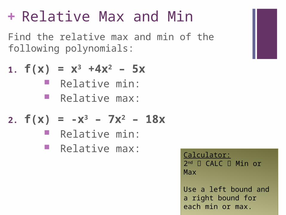
+ Relative Max and MinFind the relative max and min of the following polynomials:
1. f(x) = x3 +4x2 – 5x Relative min: Relative max:
2. f(x) = -x3 – 7x2 – 18x Relative min: Relative max:
Calculator:2nd CALC Min or Max
Use a left bound and a right bound for each min or max.

+Finding Zeros
When a Polynomial is in factored form, it is easy to find the zeros, or where the graph crosses the x-axis.
EX: Find the Zeros of y = (x+4)(x – 3)
+Factor Theorem
The Expression x – a is a linear factor of a polynomial if and only if the value a is a zero of the related polynomial function.

+Find the Zeros
Find the Zeros of the Polynomial Function.
1. y = (x – 2)(x + 1)(x + 3)
2. y = (x – 7)(x – 5)(x – 3)

+Writing a Polynomial Function
Give the zeros -2, 3, and -1, write a polynomial function. Then classify it by degree and number of terms.
Give the zeros 5, -1, and -2, write a polynomial function. Then classify it by degree and number of terms.

+Repeated Zeros
A repeated zero is called a MULITIPLE ZERO.
A multiple zero has a MULTIPLICITY equal to the number of times the zero repeats.

+Find the Multiplicity of a Zero
Find any multiple zeros and their multiplicity
y = x4 + 6x3 + 8x2
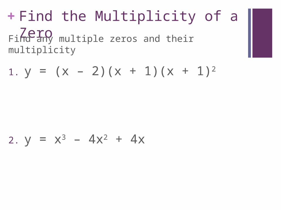
+Find the Multiplicity of a Zero
Find any multiple zeros and their multiplicity
1. y = (x – 2)(x + 1)(x + 1)2
2. y = x3 – 4x2 + 4x

+6.3 Dividing Polynomials

+Vocabulary
Dividend: number being divided
Divisor: number you are dividing by
Quotient: number you get when you divide
Remainder: the number left over if it does not divide evenly
Factors: the DIVISOR and QUOTIENT are FACTORS if there is no remainder

+Long Division
Divide WITHOUT a calculator!!
1. 2.
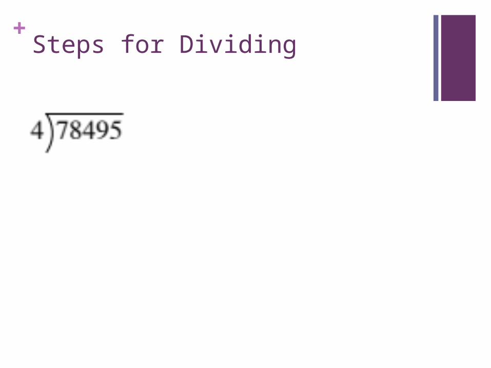
+Steps for Dividing
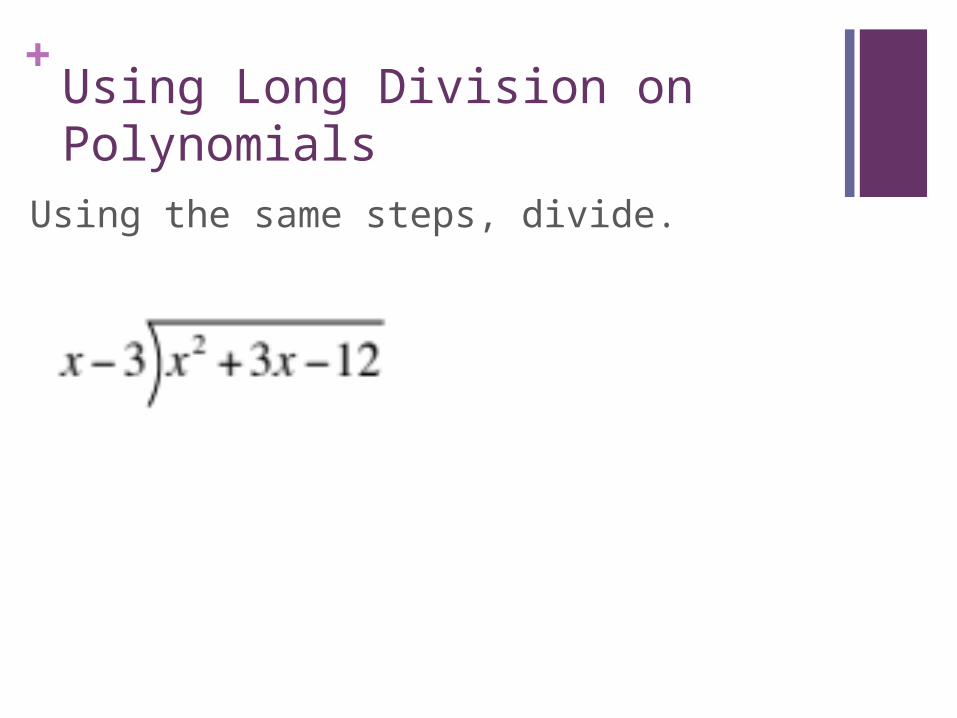
+Using Long Division on Polynomials
Using the same steps, divide.

+Using Long Division on Polynomials
Using the same steps, divide.

+Using Long Division on Polynomials
Using the same steps, divide.

+Synthetic Division

+Synthetic Division
Step 1: Switch the sign of the constant term in the divisor. Write the coefficients of the polynomial in standard form.
Step 2: Bring down the first coefficient.
Step 3: Multiply the first coefficient by the new divisor.
Step 4: Repeat step 3 until remainder is found.

+Example
Use Synthetic division to divide
3x3 – 4x2 + 2x – 1 by x + 1

+Example
Use Synthetic division to divide
X3 + 4x2 + x – 6 by x + 1

+Example
Use Synthetic division to divide
X3 + 3x2 – x – 3 by x – 1

+Remainder Theorem
Remainder Theorem: If a polynomial P(x) is divided by (x – a), where a is a constant, then the remainder is P(a).

+Using the Remainder Theorem
Find P(-4) for P(x) = x4 – 5x2 + 4x + 12.

+6.4 Solving Polynomials by Graphing

+Solving by Graphing: 1st Way
Solutions are zeros on a graph
Step 1: Solve for zero on one side of the equation.
Step 2: Graph the equation
Step 3: Find the Zeros using 2nd CALC
(Find each zero individually)

+
Step 1: Graph both sides of the equal sign as two separate equations in y1 and y2.
Use 2nd CALC Intersect to find the x values at the points of intersection
Solving by Graphing: 2nd Way

+Solve by Graphing
x3 + 3x2 = x + 3
x3 – 4x2 – 7x = -10
+Solve by Graphing
x3 + 6x2 + 11x + 6 = 0

+Solving by Factoring

+Factoring Sum and Difference
Factoring cubic equations:
Note: The second factor is prime (cannot be factored anymore)

+ Factor:
1) x3 - 8
2) 27x3 + 1

+You Try! Factor:
1) x3 + 64
2) 8x3 - 1
3) 8x3 - 27

+
Solving a Polynomial Equation

+Solving By Factoring
Remember: Once a polynomial is in factored form, we can set each factor equal to zero and solve.
4x3 – 8x2 + 4x = 0
+Solve by factoring:
1. 2x3 + 5x2 = 7x
2. x2 – 8x + 7 = 0

+Using the patterns to Solve
So solve cubic sum and differences use our pattern to factor then solve.
X3 – 8 = 0

+Using the patterns to Solve
x3 – 64 = 0

+Using the patterns to Solve
x3 + 27 = 0

+
Factoring by Using Quadratic Form

+Factoring by using Quadratic Formx4 – 2x2 – 8

+Factoring by using Quadratic Formx4 + 7x2 + 6

+Factoring by using Quadratic Formx4 – 3x2 – 10

+Solving Using Quadratic Form
x4 – x2 = 12

+
6.5 Theorems About Roots

+The Degree
Remember: the degree of a polynomial is the highest exponent.
The Degree also tells us the number of Solutions (Including Real AND Imaginary)

+Solutions/Roots
How many solutions will each equation have? What are they?
1. x3 – 6x2 – 16x = 0
2. x3 + 343 = 0
+Solving by Graphing
Solving by Graphing ONLY works for REAL SOLUTIONS. You cannot find Imaginary solutions from a Graph.
Roots: This is another word for zeros or solutions.

+Rational Root Theorem
If p/q is a rational root (solution) then:
p must be a factor of the constant
and
q must be a factor of the leading coefficient

+Example
x3 – 5x2 - 2x + 24 = 0
Lets look at the graph to find the solutions
Factored (x + 2)(x – 3)(x – 4) = 0
Note: Roots are all factors of 24 (the constant term) since a = 1.

+Example
24x3 – 22x2 - 5x + 6 = 0
Lets look at the graph to find the solutions:
Factored (x + ½ )(x – ⅔)(x – ¾ ) = 0 1,2, and 3 (the numerators) are all factors of 6 (the
constant).
2, 3, and 4 (the denominators) are all factors of 24 (the leading coefficient).

+ 8) x3 – 5x2 + 7x – 35 = 0

+ 10) 4x3 + 16x2 -22x -10 = 0
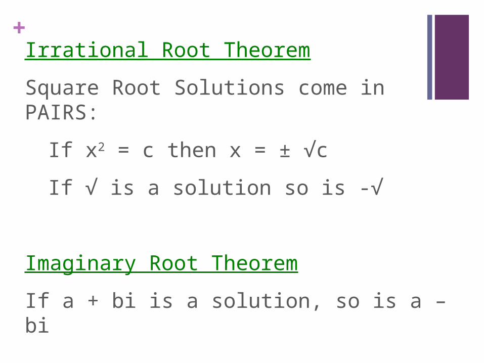
+Irrational Root Theorem
Square Root Solutions come in PAIRS:
If x2 = c then x = ± √c
If √ is a solution so is -√
Imaginary Root Theorem
If a + bi is a solution, so is a – bi

+Recall
Solve the following by taking the square root:
X2 – 49 = 0
X2 + 36 = 0
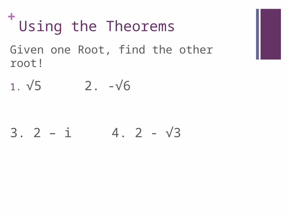
+Using the Theorems
Given one Root, find the other root!
1. √5 2. -√6
3. 2 – i 4. 2 - √3

+Zeros to Factors
If a is a zero, then (x – a) is a factor!!
When you have factors
(x – a)(x – b) = x2 + (a+b)x + (ab)
SUM PRODUCT

+Examples
1. Find a 2nd degree equation with roots 2 and 3
(x - _______)(x - ______)
2. Find a 2nd degree equation with roots -1 and 6

+Example
1. Find a 2nd degree equation with roots ±√7

+Examples
1. Find a 2nd degree equation with roots ±2√5
2. Find a 2nd degree equation with roots ±6i

+Examples
Find a 2nd degree equation with a root of 7 + i

+Example
Find a 3rd degree equation with roots 4 and 3i
(x - _______)(x - ______)(x - ______)

+Example
Find a third degree polynomial equation with roots 3 and 1 + i.