+ model article in press - university of adelaide · article in press 1 2 correction of ... (lake,...

ARTICLE IN PRESS

1

2

3

45

6

7

8

9

10111213141516171819202122232425

26

27

28

29303132

www.elsevier.com/locate/petrol

+ model

Journal of Petroleum Science and E

F

Correction of basic equations for deep bed filtration with dispersion

J.E. Altoe F. a, P. Bedrikovetsky a,*, A.G. Siqueira b, A.L.S. de Souza b, F.S. Shecaira b

a Department of Petroleum Exploration and Production Engineering, North Fluminense State University Lenep/UENF,

Rod. Amaral Peixoto, km 163 – Av. Brenand, s/n8 Imboacica – Macae, RJ 27.925-310, Brazilb Petrobras/Cenpes, Cidade Universitaria Q.7, Ilha Do Fundao, 21949-900 – Rio De Janeiro — RJ, Brazil

Accepted 4 November 2005
O
RRECTED PROAbstract

Deep bed filtration of particle suspensions in porous media occurs during water injection into oil reservoirs, drilling fluid

invasion into reservoir productive zones, fines migration in oil fields, bacteria, virus or contaminant transport in groundwater,

industrial filtering, etc. The basic features of the process are advective and dispersive particle transport and particle capture by the

porous medium.

Particle transport in porous media is determined by advective flow of carrier water and by hydrodynamic dispersion in micro-

heterogeneous media. Thus, the particle flux is the sum of advective and dispersive fluxes. Transport of particles in porous media is

described by an advection–diffusion equation and by a kinetic equation of particle capture. Conventional models for deep bed

filtration take into account hydrodynamic particle dispersion in the mass balance equation but do not consider the effect of

dispersive flux on retention kinetics.

In the present study, a model for deep bed filtration with particle size exclusion taking into account particle hydrodynamic

dispersion in both mass balance and retention kinetics equations is proposed. Analytical solutions are obtained for flows in infinite

and semi-infinite reservoirs and in finite porous columns. The physical interpretation of the steady-state flow regimes described by

the proposed and the traditional models favours the former.

Comparative matching of experimental data on particle transport in porous columns by the two models is performed for two sets

of laboratory data.

D 2005 Published by Elsevier B.V.

Keywords: Deep bed filtration; Dispersion; Suspension; Governing equations; Modelling; Porous media; Emulsion

333435363738

NCO1. Introduction

Severe injectivity decline during sea/produced water

injection is a serious problem in offshore waterflood

projects. The permeability impairment occurs due to

capture of particles from injected water by the rock.
U 3940414243
0920-4105/$ - see front matter D 2005 Published by Elsevier B.V.

doi:10.1016/j.petrol.2005.11.010

* Corresponding author. Tel.: +55 22 27733391; fax: +55 22

27736565.

E-mail addresses: [email protected], [email protected]

(P. Bedrikovetsky).

The reliable modelling-based prediction of injectivity

decline is important for the injected-water-treatment

design, for injected water management (injection of

sea- or produced water, their combinations, water fil-

tering), etc.

The formation damage induced by penetration of

drilling fluid into a reservoir also occurs due to particle

capture by rocks and consequent permeability reduc-

tion. Other petroleum applications include sand produc-

tion control, fines migration and deep bed filtration in

gravel packs.

ngineering xx (2005) xxx–xxx

PETROL-01339; No of Pages 17

T

ARTICLE IN PRESS

44454647484950515253545556575859606162636465666768697071727374757677787980818283848586878889909192939495

96979899100101102103104105106107108109110111112113114115116

117

118119120121122123

124125126127128129130131

132

133134135136137138139140141142

J.E. Altoe F. et al. / Journal of Petroleum Science and Engineering xx (2005) xxx–xxx2

UNCORREC

The basic equations for deep bed filtration taking

into account advective particle transport and the kinet-

ics of particle retention, and neglecting hydrodynamic

dispersion have been derived essentially following the

filtration equation proposed by Iwasaki (1937). A num-

ber of predictive models have been presented in the

literature (Sharma and Yortsos, 1987a,b,c; Elimelech et

al., 1995; Tiab and Donaldson, 1996, Khilar and Fogler,

1998; Logan, 2001). The equations allow for various

analytical solutions, which have been used for the

treatment of laboratory data and for prediction of po-

rous media contamination and clogging (Herzig et al.,

1970; Pang and Sharma, 1994; Wennberg and Sharma,

1997; Bedrikovetsky et al., 2001, 2002).

However, particle dispersion in heterogeneous po-

rous media is important for both small and large scales

(Lake, 1989; Jensen et al., 1997). The typical core sizes

in laboratory experiments are small, and hence the

Peclet number is relatively high. The typical dispersiv-

ity values for large formation scales are high, and

consequently the Peclet number may also take high

values. The Peclet number for either situation may

amount up to 10–20.

The effect of dispersion on deep bed filtration is

particularly important near to wells, where the disper-

sivity may already arise to the bed scale, and the forma-

tion damage occurs in one two-meter neighbourhood.

Therefore, several deep bed filtration studies take

into account dispersion of particles (Grolimund et al.,

1998; Kretzschmar et al., 1997; Bolster et al., 1998;

Unice and Logan, 2000; Logan, 2001; Tufenkji et al.,

2003). A detailed description of such early work is

presented in the review paper by Herzig et al. (1970).

The models developed account for particle dispersion in

the mass balance for particles but do not consider the

dispersion flux contribution to the retention kinetics.

In the present study, the proposed deep bed filtration

model takes into account dispersion in both the equa-

tion of mass balance and in that of capture kinetics.

Several analytical models for constant filtration coeffi-

cient and for dynamic blocking filtration coefficient

have been developed. If compared with the traditional

model, the proposed model exhibits more realistic

physics behaviour. The difference between the tradi-

tional and proposed model is significant for small Pec-

let numbers.

The structure of the paper is as follows. In Section 2

we formulate the corrected model for deep bed filtration

of particulate suspensions in porous media accounting

for hydrodynamic dispersion of suspended particles.

The dispersion-free deep bed filtration model is pre-

sented in Section 3 as a particulate case of the general

ED PROOF

system with dispersion. The analytical models for flow

in infinite and semi-infinite reservoirs for constant fil-

tration coefficient are presented in Sections 4 and 5,

respectively. An analytical solution for deep bed filtra-

tion in semi-infinite reservoirs with the fixed inlet

concentration is given in Section 6. Analytical steady

state solution for laboratory coreflood in discussed in

Section 7. The analytical models allow for laboratory

data treatment (Section 8). Travelling wave flow

regimes for dynamic blocking filtration coefficient are

described in Section 9. In Section 10, three dimensional

equations for deep bed filtration with dispersion are

derived. Mathematical details of the derivations are

presented in Appendices. Dimensionless form of gov-

erning equations and initial-boundary conditions are

given in Appendix A. The transient solutions for flow

in infinite and semi-infinite reservoirs and constant

filtration coefficient are derived in Appendices B, C

and D. Appendix E contains derivations for steady state

solution in a finite core. Appendix F contains deriva-

tions for travelling wave flow.

2. Model formulation

Let us derive governing equations for deep bed

filtration taking into account particle dispersion. The

usual assumptions of constant suspension density and

porosity for low particle concentrations are adopted.

The balance equation for suspended and retained parti-

cles (Iwasaki, 1937; Herzig et al., 1970) is:

B

Bt/cþ rð Þ þ Bq

Bx¼ 0 ð1Þ

Here, the concentration c is a number of suspended

particles per unit volume of the fluid, and the retained

particle concentration r is a number of captured parti-

cles per unit volume of the rock.

The particle flux q consists of the advective and

dispersive components:

q ¼ Uc� DBc

Bxð2Þ

D ¼ aDU ð3Þ

Here the dispersion coefficient D is assumed to be

proportional to the flow velocity U, and the proportion-

ality coefficient aD is called the longitudinal dispersiv-

ity (Lake, 1989; Nikolaevskij, 1990; Sorbie, 1991).

Let us consider the following physical model for the

size exclusion particle capture in porous media (Santos

and Bedrikovetsky, 2005). Particles are not captured

during flow through the pore system, but there is a

T

F

ARTICLE IN PRESS

143144145146147148149150151152153154155156157158159160161162163164165166

167168169170171172173174175176

177178179180181182183184185186187188189190

191192193194195196197198199200201202203204205206207208209210211212213214215216217218219220221222223224

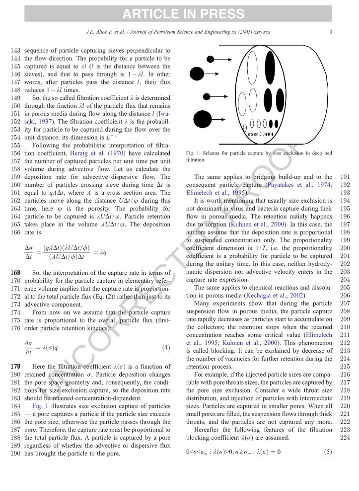
Fig. 1. Schema for particle capture by size exclusion in deep bed

filtration.

J.E. Altoe F. et al. / Journal of Petroleum Science and Engineering xx (2005) xxx–xxx 3

UNCORREC

sequence of particle capturing sieves perpendicular to

the flow direction. The probability for a particle to be

captured is equal to kl (l is the distance between the

sieves), and that to pass through is 1�kl. In other

words, after particles pass the distance l, their flux

reduces 1�kl times.

So, the so called filtration coefficient k is determined

through the fraction kl of the particle flux that remains

in porous media during flow along the distance l (Iwa-

saki, 1937). The filtration coefficient k is the probabil-

ity for particle to be captured during the flow over the

unit distance; its dimension is L�1.

Following the probabilistic interpretation of filtra-

tion coefficient, Herzig et al. (1970) have calculated

the number of captured particles per unit time per unit

volume during advective flow. Let us calculate the

deposition rate for advective–dispersive flow. The

number of particles crossing sieve during time Dt is

equal to qADt, where A is a cross section area. The

particles move along the distance UDt /u during this

time, here u is the porosity. The probability for

particle to be captured is kUDt /u. Particle retention

takes place in the volume AUDt /u. The deposition

rate is

DrDt

¼ qADtð Þ kUDt=/ð ÞAUDt=/ð ÞDt ¼ kq

So, the interpretation of the capture rate in terms of

probability for the particle capture in elementary refer-

ence volume implies that the capture rate is proportion-

al to the total particle flux (Eq. (2)) rather than just to its

advective component.

From now on we assume that the particle capture

rate is proportional to the overall particle flux (first-

order particle retention kinetics):

BrBt

¼ k rð Þq ð4Þ

Here the filtration coefficient k(r) is a function of

retained concentration r. Particle deposition changes

the pore space geometry and, consequently, the condi-

tions for size exclusion capture, so the deposition rate

should be retained-concentration-dependent.

Fig. 1 illustrates size exclusion capture of particles

— a pore captures a particle if the particle size exceeds

the pore size, otherwise the particle passes through the

pore. Therefore, the capture rate must be proportional to

the total particle flux. A particle is captured by a pore

regardless of whether the advective or dispersive flux

has brought the particle to the pore.

ED PROO

The same applies to bridging build-up and to the

consequent particle capture (Payatakes et al., 1974;

Elimelech et al., 1995).

It is worth mentioning that usually size exclusion is

not dominant in virus and bacteria capture during their

flow in porous media. The retention mainly happens

due to sorption (Kuhnen et al., 2000). In this case, the

authors assume that the deposition rate is proportional

to suspended concentration only. The proportionality

coefficient dimension is 1 /T, i.e. the proportionality

coefficient is a probability for particle to be captured

during the unitary time. In this case, neither hydrody-

namic dispersion nor advective velocity enters in the

capture rate expression.

The same applies to chemical reactions and dissolu-

tion in porous media (Kechagia et al., 2002).

Many experiments show that during the particle

suspension flow in porous media, the particle capture

rate rapidly decreases as particles start to accumulate on

the collectors; the retention stops when the retained

concentration reaches some critical value (Elimelech

et al., 1995; Kuhnen et al., 2000). This phenomenon

is called blocking. It can be explained by decrease of

the number of vacancies for further retention during the

retention process.

For example, if the injected particle sizes are compa-

rable with pore throats sizes, the particles are captured by

the pore size exclusion. Consider a wide throat size

distribution, and injection of particles with intermediate

sizes. Particles are captured in smaller pores. When all

small pores are filled, the suspension flows through thick

throats, and the particles are not captured any more.

Hereafter the following features of the filtration

blocking coefficient k(r) are assumed:

0brbrm : k rð ÞN0; rzrm : k rð Þ ¼ 0 ð5Þ

T

ARTICLE IN PRESS

225226

227

228229

230

231

232233234235236237

238239240241242

243244245246247248249250251252253254255256257258259

260

261262263264265266267268269270271272273

274275276277278279280281282283

284285286287288289290291292293294295296297298299300301302303304305306307308309310311312

313314315316317

318319320321322

323324


UNCORREC

The important particular case of Eq. (5) is the linear

filtration coefficient

k rð Þ ¼ k0 1� brð Þ ð6Þ

so called Langmuir blocking function (Kuhnen et al.,

2000). It is typical where the capture is realized by a

mono-layer adsorption.

This case corresponds to the situation where one

vacancy can be filled by one particle. So, retention of

some particles results in filling of the same number of

vacancies, i.e. the total of deposited particle concentra-

tion r(x, t) and the vacant pore concentration h(x, t) is

equal to initial concentration of vacancies h(x,0):

h x; tð Þ ¼ h x; 0ð Þ � r x; tð Þ ð7Þ

The capture rate is proportional to the product of

particle flux and vacancy concentration (acting mass

law). Using Eq. (7), we obtain:

BrBt

¼ k0 1� rh x; 0ð Þ

� �q ð8Þ

The filtration function k(r) depends on porous media

structure. Therefore, for heterogeneous porous media

where initial vacancy concentration depends on x, the

filtration function is x-dependent: k=k(r,x). Further inthe paper we assume a uniform initial vacancy concen-

tration and use the dependency k =k(r).So, the Langmuir linear blocking function (Eq. (6))

corresponds to bone particle – one poreQ kinetics [Eq.

(8)]. The comparison of formulae Eqs. (8) and (4)

results in Eq. (6).

If k0 in Eq. (8) is also a function of r, the blocking

filtration coefficient k(r) is non-linear.Darcy’s law for suspension flow in porous media

includes the effect of permeability decline during par-

ticle retention:

U ¼ � k0k rð Þl

Bp

Bxð9Þ

k rð Þ ¼ 1

1þ brð10Þ

Here k(r) is called the permeability reduction function,

and b is the formation damage coefficient.

Eqs. (1), (2), (4) and (9) form a closed system of four

equations that govern the colloid filtration with size

exclusion particle capture in porous media. The

unknowns are suspended concentration c, deposited

r, particle flux q and pressure p.

The independence of the filtration and dispersion

coefficients of pressure allows separation of Eqs. (1),

(2) and (4) from Eq. (9), which means that the sus-

pended and retained concentrations and the particle flux

ED PROOF

can be found from the system of Eqs. (1), (2) and (4)

and then the pressure distribution can be found from

Eq. (9).

Form of the system of governing equations in

non-dimensional co-ordinates is presented in Appen-

dix A, (Eqs. (A-2)–(A-5)). The system contains the

dimensionless parameter eD that is the inverse to the

Peclet number; it is equal to the dispersion-to-advective

flux ratio (Nikolaevskij, 1990). From Eq. (3) it follows

that:

eD ¼ 1

Pe¼ D

LU¼ aD

Lð11Þ

The dispersion–advective ratio eD is equal to the ratio

between the micro heterogeneity size aD (dispersivity)

and the reference size of the boundary problem L.

Let us estimate the contribution of dispersion to the

total particle flux (Eq. (2)). In the majority of papers,

deep bed filtration model has been modelled under the

laboratory floods conditions, where homogeneous sand

columns are employed (Elimelech et al., 1995; Unice

and Logan, 2000; Tufenkji et al., 2003). On the core

scale in homogeneous cores, we have L~0.1 m,

aD~0.001 m, eD~0.01, and hence the dispersion can

be neglected. In natural heterogeneous cores, eD can

amount to 0.1 or more, and dispersion should be taken

into account (Lake, 1989; Bedrikovetsky, 1993). In a

well neighbourhood, the reference radius of formation

damage zone is 1 m, the heterogeneity reference size is

also 1 m, so eD has order of magnitude of unity.

The dispersivity aD can reach several tens or even

hundreds of meters at formation scales (Lake, 1989;

Jensen et al., 1997); thus, the dimensionless dispersion

can have the order of magnitude of unity, and hence

hydrodynamic dispersion should be taken into account.

Now we formulate one dimensional problem for

suspension injection into a porous core/reservoir.

The absence of suspended and retained particles in

porous media before the injection is represented by the

initial conditions:

t ¼ 0 : c ¼ r ¼ 0 ð12ÞFixing the inlet particle flux during the injection of

particulate suspension in a reservoir determines the

boundary condition:

x ¼ 0 : Uc� DBc

Bx¼ c0U ð13Þ

Sometimes the dispersive term in the boundary con-

dition (Eq. (13)) is neglected (van Genuchten, 1981 and

Nikolaevskij, 1990):

x ¼ 0 : c ¼ c0 ð14Þ

T

ARTICLE IN PRESS

325326327328329330331332333

334335336337338

339

340341342343

344345346347348349350351352353354355356357358359360361362363364365366367368369370371372

373374375376377378379380381382383384385386387388389390391392393394395396397398399400401402403

404

405406407408409

410411

412413414415


UNCORREC

The particle motion in porous media can be decom-

posed into an advective flow with constant velocity and

the dispersive random walks around the front that

moves with advective velocity (Kampen, 1984). It is

assumed that once a particle leaves the core outlet by

advection it cannot come back by dispersion. This

assumption leads to the boundary condition of absence

of dispersion at the core outlet (Danckwerts, 1953;

Nikolaevskij, 1990):

x ¼ L :Bc

Bx¼ 0 ð15Þ

In dimensionless coordinates (Eq. (A-1)), the pro-

posed model with a constant filtration coefficient takes

the form (Eqs. (A-10) and (11)):

BC

BTþ m

BC

BX¼ eD

B2C

BX 2� KC ð16Þ

m ¼ 1� KeD ð17Þ

Neglecting the dispersion term in the capture kinet-

ics Eqs. (16) and (17) results in:

BC

BTþ BC

BX¼ eD

B2C

BX 2� KC ð18Þ

Eq. (18) is a traditional advective–diffusive model

with a sink term. The boundary condition (Eq. (13))

fixes the inlet flux in this model.

Eq. (16) looks like the advective–diffusive model

(Eq. (18)) with advective velocity m, and seems this

velocity should appear in the expression for the inlet

flux (Eq. (13)). However, the real advective velocity in

Eq. (16) is equal to one, and the delay term �KeDappears due to the capture of particles transported by

the dispersive flux and is not a part of the flux. From

conservation law (Eqs. (1) and (A-2)) it follows that the

particle flux is continuous at the inlet; the boundary

condition for Eq. (16) should be given by Eq. (13) that

differs from the inlet boundary condition for the equiv-

alent advective–diffusive model with the advective

velocity m.Following Logan (2001), from now on the model

(Eq. (18)) will be referred to as the HLL model in order

to honour the fundamental work by Herzig et al.

(1970).

The difference between the presented and the HLL

model is the delay term KeD that appears in the advec-

tive flux velocity (Eq. (17)). This is the collective effect

of the particle dispersion and capture. Appearance of

the delay term KeD in the advective flux velocity (Eq.

(17)) is due to accounting for diffusive flux in the

capture kinetics (Eq. (2) and Eq. (4)).

ED PROOF

A delay in the particle pulse arrival to the column

effluent if compared with the tracer pulse breakthrough

was observed by Massei et al. (2002).

The length L used in dimensionless parameters (Eq.

(A-1)) is a reference size of the boundary problem. It

affects the dimensionless filtration coefficient K (Eq.

(A-1)) and the inverse to Peclet number eD, (Eq. (11))and drops out the delay term: KeD =kaD. The dimen-

sionless time T corresponding to the length L (Eq. (A-

1)) is measured in bpore volume injectedQ, which is the

common unit in laboratory coreflooding and in field

data presentation.

Also, often the injected suspension is traced, and

the particle breakthrough curves are presented togeth-

er with tracer curves (Jin et al., 1997; Ginn, 2000). In

this case, the inverse to Peclet number eD in Eq. (16)

is already known from the tracer data and it is conve-

nient to use dimensionless variables and parameters

(Eq. (A-1)).

Nevertheless, Eq. (16) depends on two independent

dimensionless parameters —eD and K.

The inverse to filtration coefficient is an average

penetration depth of suspended particles (Herzig et

al., 1970), so the inverse to reference value of filtration

coefficient 1 /k0 can be used as a reference length in

dimensionless linear co-ordinate (Eq. (A-12)). For

corresponding dimensionless variables (Eq. (A-12)),

the dimensionless K becomes equal to unit in the

case of constant filtration coefficient, and Eq. (16)

becomes dependent of one dimensionless parameter eonly, (Eq. (A-13)):

BC

BTVþ m

BC

BXV¼ e

B2C

BXV2� C ð19Þ

m ¼ 1� e; e ¼ k0aD

In the case of filtration function K =K(S), Eq. (16)

includes deposited concentration S, and the model con-

sists of two equations

BC

BTþ 1� K Sð ÞeDð Þ BC

BX¼ eD

B2C

BX 2� K Sð ÞC

BS

BT¼ K Sð Þ 1� eD

BC

BX

� �ð20Þ

for dimensionless parameters (Eq. (A-1)).

For dimensionless variables (Eq. (A-12)), eD must

be changed to e=k0aD.The HLL in this case is also obtained by neglecting

dispersion term in capture rate expression.

T

ARTICLE IN PRESS

416417

418419

420421422

423424425426427428

429430431432433434

435436437438439

440

441442443444

445446447448449450

451452453454455456457

458

459460461462463464465466467468469470471472473474475476477478479480

481482

483484485486487488489

Fig. 2. Concentration wave dynamics in an infinite reservoir by the

presented model and by the HLL model.


UNCORREC

The order of the governing system (Eq. (20)) can be

reduced by one. Introducing the function

U Sð Þ ¼Z S

0

1

K sð Þ ds ð21Þ

from Eq. (A-3) we obtain:

BU Sð ÞBT

¼ Q ð22Þ

Substitution of Eq. (22) into Eq. (A-2) results in

B

BTC þ Sð Þ þ B

BX

BU Sð ÞBT

� �¼ 0 ð23Þ

Changing order of differentiation in the second term in

the right hand side of Eq. (23) and integrating in T from

zero to T, we obtain first order partial differential

equation:

C þ S þ BU Sð ÞBX

¼ 0 ð24Þ

The integration constant that should appear in right

hand side of Eq. (24) was calculated from initial con-

ditions (Eq. (12)) — it is equal zero.

Eq. (22) becomes

BU Sð ÞBT

¼ 1� eDBC

BXð25Þ

Eqs. (24) and (25) form quasi-linear system of first

order equations modeling deep bed filtration with size

exclusion particle capture accounting for dispersion.

3. Dispersion free model

Neglecting the dispersion in Eq. (16) results in the

simplified deep bed filtration model (Sharma and Yort-

sos, 1987a,b,c; Elimelech et al., 1995; Tiab and

Donaldson, 1996):

BC

BTþ BC

BX¼ � KC ð26Þ

The boundary condition (Eq. (13)) automatically takes

the form of Eq. (14).

The solution of the dispersion-free deep bed filtra-

tion problem (Eqs. (26) (12) and (14)) is given by

C X ; Tð Þ ¼ exp � KXð Þ XVT0 XNT

�ð27Þ

Concentration is zero ahead of the concentration front

X0(T)=T. Particles arrive at the column outlet after one

pore volume injection. Once the advancing front passes

a given location, a steady concentration distribution is

immediately established behind the front.

ED PROOF

4. Transient flow in infinite reservoir

Let us consider flow in an infinite reservoir where,

initially, water with particles fills the semi-infinite res-

ervoir X b0, and clean water fills the semi-infinite

reservoir X N0. Formula for concentration wave propa-

gation (Eq. (B-2)) is presented in Appendix B.

Fig. 2 shows the concentration profiles for the times

T=0.1, 1.0 and 4.0 with eD =1.0 and K =0.5. Solid

lines correspond to the proposed model and dotted

lines correspond to the HLL model. Both models ex-

hibit advective propagation of the concentration wave

with diffusive smoothing of the initial shock; the mix-

ture zone expands with time. Suspended concentration

is zero ahead of the mixture zone. Behind the mixture

zone, concentration does not vary along the reservoir

and exponentially decays with time due to deep bed

filtration with a constant filtration coefficient. One can

observe a delay in the concentration front propagation

for the proposed model (Eq. (16)) if compared with the

HLL model (Eq. (18)). The difference in the profiles in

the two models appears in the mixture zone, while the

concentrations ahead of and behind the mixture zone

coincide for both models.

5. Analytical model for suspension injection into

semi-infinite reservoir

In this section we consider the particulate suspension

injection into a semi-infinite reservoir, X N0. The ex-

pression for suspension concentration (Eq. (C-2)) is

presented in Appendix C.

Fig. 3 epicts particle flux profiles for the dispersi

shows the concentration profiles at the moments

T=0.5, 1.0, 2.0 and 6.0 as obtained by explicit formula

T

ARTICLE IN PRESS

490491492493494495496497498499500501502503504505506507508509510511512513514

515516517518519520521522523524525526527528529530531532533534535536537538539540541542543544545546547548549550

Fig. 3. Dynamics of concentration waves in a semi-infinite reservoir.


RREC

(Eq. (C-2)). The envelope curve corresponds to the

steady-state solution (Eq. (C-5)). Furthermore, for any

moment T there exists such position of a mixture zone

X0(T) that the transient and steady-state profiles behind

the zone (X bX0(T)) almost coincide. Once the transi-

tion zone passes a given location, the steady-state sus-

pended concentration distribution is established behind.

After establishing the steady state, all newly arrived

particles are captured by the rock, and the suspended

concentration is time-independent.

The term bsteady stateQ is applied to the suspended

concentration only. The retained concentration

increases during the flow.

The particle flux profile in the steady-state regime

(Eq. (C-6)) shows that the kth fraction of the particle

flux is captured under the steady-state conditions, and

(1�k)th fraction passes through. The result must be

independent of the particle flux partition into the ad-

vective and dispersive parts, i.e. the formula for the

steady-state flux profile must not contain the dispersion

coefficient (Eq. (C-6)).

Fig. 4 depicts particle flux profiles for the disper-

sion-free model (solid line) and for the proposed model

using the solution (Eq. (C-5)) (dotted line) for

eD=0.002 and K =1. The suspended concentration

UNCO

Fig. 4. Particle flux profile for T=0.5 (semi-infinite reservoir) by the

proposed model and the dispersion-free model.

ED PROOF

and the particle flux coincide for dispersion-free flow,

and the profile is discontinuous. The introduction of

particle dispersion leads to smoothing the shock out.

The larger is the dispersion coefficient, the wider is the

smoothed zone around the shock.

Fig. 5 presents particle flux histories at the point

X =1 in a semi-infinite reservoir for the dispersion-free

case (curve eD =0) and three different dispersion values

eD=0.01, 0.1 and 0.5. On the one side, the higher is

the dispersion, the larger is the delay in the arrival of the

concentration front. On the other side, the larger is

the dispersion, the wider is the mixture zone about the

shock. Thus, the effect of the delay in advection com-

petes with that of the dispersion zone expansion. Fig. 5

shows fast breakthrough for large dispersion values.

Let us compare the stationary particle flux profiles

behind the moving mixture zone as obtained by the

proposed and HLL models. The solution can be

obtained from Eq. (C-2) by setting m =1 and tending

T to infinity. The calculation of the flux profile shows

that it is dispersion-dependent.

The asymptotic steady-state particle flux profile

(Eq. (C-6)) for the presented model coincides

with that for the dispersion-free model and is

dispersion-independent.

The comparative results are displayed in Fig. 6. The

flux is equal to 0.37 at X =1 for both the proposed and

dispersion-free models. The HLL model profiles were

calculated for eD =0.1, 1.0 and 3.0; the corresponding

particle fluxes at X =1 were found to be 0.40, 0.54 and

0.65, respectively.

The directions of diffusive and advective fluxes co-

incide. Therefore, inclusion of the diffusive flux into the

particle capture rate (Eq. (4)) increases the retention, and

the flux profile as calculated by the proposed model is

located below that as obtained by HLL model (Fig. 6).

Fig. 5. Particle flux history at the point X =1 in semi-infinite reservoir

for different dispersion coefficients.

T

OF

ARTICLE IN PRESS

551552553554555556557558559560561562563564565566567568

569570571572573574

575576

577578579580581582583

Fig. 6. Steady-state particle flux profiles for the dispersion-free case

and by the presented model (the same solid curve) and by the HLL

model with eD =0.1, eD =1.0 and eD =3 (dotted, dot-and-dash and

dashed lines, respectively).

Fig. 8. Comparison between steady-state concentration profiles for

deep bed filtration in a semi-infinite reservoir taking into account and

neglecting dispersion in the inlet boundary conditions.


EC

One may notice a significant difference between the

two profiles as calculated by the proposed and the HLL

model for large dimensionless dispersion (eD =1.0 and

3.0); the difference is negligible for eD less than 0.1.

The dependence of the particle flux at X =1 on the

dimensionless dispersion eD is plotted in Fig. 7 for

the proposed model (solid line) and the HLL model

(dashed line). As mentioned before, the particle flux

predicted by the proposed model is independent of

dispersion for the steady-state regime (Eq. (C-6)),

which implies that the solid line is horizontal.

Consider the asymptotic case where the Peclet num-

ber vanishes. As eDH1, the flux in the HLL model

tends to unity; hence the steady-state flux is constant

along the column and no particle is captured, which is

unphysical. For large dispersion, the advective flux is

relatively low; the capture rate in the HLL model is

proportional to the advective flux and, therefore, is also

UNCORR 584585586587588589590591592593594595

596

597598599

Fig. 7. Effect of dispersion on the flux at X= 1 for the steady-state

mode in a semi-infinite reservoir for proposed and HLL models.

ED PROlow. Thus, particle capture vanishes as eDH1. No

particle retention occurs when the dispersive mass

transfer dominates over the advection.

The obtained contradiction occurs because the HLL

model does not account for capture of particles trans-

ported by dispersive flux (Fig. 8).

6. Filtration in semi-infinite reservoir with simplified

inlet boundary conditions

Let us discuss the case where dispersion is neglected

in the inlet boundary condition (Eq. (14)). The exact

solution is obtained in Appendix D, (Eq. (D-1)).

The concentration profile in steady-state regime (Eq.

(D-2)) coincides with the concentration profile for the

dispersion-free model. The simplified inlet boundary

condition (Eq. (14)) is the same as the one for the

dispersion-free model. Hence, the introduction of dis-

persion into the deep bed filtration model while keeping

the same boundary condition (Eq. (14)) does not change

the asymptotic profile of the suspended concentration.

Fig. 6 shows steady-state concentration profiles for

the simplified inlet boundary condition, given by Eq.

(D-2) (solid line) and for the complete inlet boundary

condition, given by Eq. (C-5) (dotted curves). Three

dotted curves correspond to eD =0.1, 1.0 and 3.0. The

inlet concentration for dotted lines is always less than

unity. The higher is the dispersion the lower is the

stationary concentration under the fixed inlet flux.

7. Steady-state solution for filtration in finite cores

The expression for the particle flux profile in steady-

state regime (Eq. (E-2)) coincides with the flux profile

behind the mixture zone in semi-infinite media. The

T

ARTICLE IN PRESS

600601602603604605606607608609610611612613614615616617618619620621622623624625626627628629

630

631632

633634

635636637638639640641642643644645646647648649650651652653654655656657658659660661662663664665666

Fig. 9. Steady-state suspended concentration profiles for filtration in a

limited core for eD =0, 0.1, 1.0 and 3.0 (solid, dotted, dashed and dot-

and-dash lines, respectively).

Fig. 10. Effect of dispersion on the particle flux at the core outlet fo

steady-state flows.


UNCORREC

concentration profiles are different because the bound-

ary condition of the dispersion absence is set at the core

outlet X =1 for the finite cores and at XYl for semi-

infinite media.

The inlet concentration (Eq. (E-4)) is less than unity.

It decreases as dispersion increases. By letting eDYlin Eq. (E-4), we find that the inlet concentration tends

to exp(�K), which is the outlet concentration (Eq. (E-

5)). Hence, as dispersion tends to infinity, the sus-

pended concentration profile becomes uniform.

Fig. 9 shows suspended concentration profiles for

eD=0.1, 1.0 and 3.0. The inlet concentration for eD =0.1is equal to 0.91. For eD =3.0 the profile is almost uniform.

It is important to emphasize that the outlet concentra-

tion (Eq. (E-5)) is independent of the dispersion coeffi-

cient and is determined by the filtration coefficient only.

This fact is in agreement with the presented above

interpretation of the filtration coefficient: kl is the prob-ability for a particle to be captured by the sieve. The

outlet concentration coincides with the particle flux due

to the outlet boundary condition (Eq. (A-7)). Therefore,

the outlet concentration under the steady-state condi-

tions must be determined by the probability for a particle

to be captured and must be independent of dispersion.

The outlet concentration predicted by the HLL

model depends on the dispersion coefficient.

It is worth mentioning that the retention profile (Eq.

(E-6)) is dispersion independent. This is because the

capture rate is proportional to the total particle flux

(Eq. (E-2)).

8. Treatment of laboratory data

The formula for steady state limit of the outlet

concentration (Eq. (E-5)) allows determining the filtra-

ED PROOF

tion coefficient from the asymptotic value of the break-

through curve. From Eq. (E-5) it follows that

K ¼ � lnC 1ð Þ ð28Þ

Formula Eq. (28) coincides with that for determining

the filtration coefficient from the asymptotic value of

the breakthrough curve using the dispersion-free model

(Eq. (26)), see (Pang and Sharma, 1994). The disper-

sion acts only in the concentration front neighbourhood,

the asymptotic value for the breakthrough concentration

is dispersion-independent.

Let us find out which model provides better fit to the

experimental data. First, we determine the intervals for

the test parameters where the difference between the

modelling data by the two models is significant.

The proposed and HLL models differ by the delay

term KeD in the advective velocity. The models coincide

as eD =0. Hence, the larger is the dispersivity, the highershould be the difference between the two models.

Fig. 10 shows the core outlet flux for the steady-state

regime with different K and eD as calculated by the

proposed model (solid line) and the HLL model

(dashed line). The marked points on dashed curves

correspond to the value of eD where the difference

between the proposed and HLL models starts to exceed

10%. For K =4, 1 and 0.55, the 10%, the difference

between the outlet fluxes can be observed for eD greater

than 0.006, 0.13 and 1.74, respectively. The value K =4

is typical for seawater injected in medium permeability

cores. The value K =0.55 is typical for virus transport

in highly permeable porous columns. The typical core

size L=0.1 m. So, in order to validate the proposed and

HLL models, one should perform laboratory coreflood

with seawater in cores with dispersivity exceeding

r

TED PROOF

ARTICLE IN PRESS

685686687688689690691692693694695696697698699700701702703704705706707708709710711712713714715716717718719720721722723724

725726727728729730731732733734

t1.1

t1.3

t1.4t1.5t1.6t1.7t1.8t1.9

Fig. 11. Matching the breakthrough curves by the proposed and the

HLL models (solid and dashed lines, respectively).


ORREC

10�3 m; the core dispersivity for virus transport should

exceed 0.2 m.

In papers by Ginn, 2000 and Jin et al., 1997, the

outlet concentrations during the injection of particulate

suspensions into sand porous columns were measured

in laboratory tests. Flow experiments on the transport of

oocysts bacteria and pathogenic viruses were carried

out in these studies. Laboratory test parameters are

presented in Table 1, where the first and the second

lines correspond to tests presented in Ginn, 2000, four

other tests are taken from the paper by Jin et al., 1997.

The breakthrough curves in Fig. 11a, b correspond to

tests 2 and 3. The filtration coefficients are calculated

from the asymptotic values C(X =1, TYl) by Eq.

(28) and are presented in Table 2.

In the laboratory tests in both works, the injected

water was traced, and the tracer outlet concentrations

were measured. Chloride and bromide tracers were used

in order to determine the dispersion coefficient. The

particle dispersion was assumed to be equal to the tracer

dispersion. The values of dispersion coefficient are

given in Table 1. Comparing the eD values in Fig. 10

and those in Table 1, one could conclude that there

should be no significant difference between the pro-

posed and HLL models for low values of dispersion in

the laboratory tests.

Matching the laboratory data in limited cores by the

analytical model for flow in a semi-infinite reservoir

was suggested by Unice and Logan (2000). Fig. 11a

and b depict breakthrough curves calculated by the

analytical model (Eq. (C-2)) using the values of Kand eD from Tables 1 and 2.

From Fig. 11a and b it is apparent that both models

describe the experimental data equally well.

The difference between the filtration coefficients as

predicted by the different models (second and third

columns of the table) is not very high due to low

dispersion of the porous media used in laboratory

tests. A typical value of the filtration coefficient in

Table 2 is K =1.4, and hence the two models would

UNC 735736737738739740741742743744745746

Table 1

Summary of experiments by Ginn (2002) and Jin et al. (1997)

Test no Column

length L

(cm)

Flow

rate Jw(cm/h)

Dispersion

coeff. D

(cm2/h)

Dispersivity

aD (cm)

Dimensionless

dispersion eD

Exp.1 10.0 29.6 7.70 0.26 0.026

Exp.2 10.0 2.96 0.53 0.18 0.018

Exp.3 20.0 3.35 1.23 0.37 0.02

Exp.4 20.0 3.19 1.13 0.35 0.02

Exp.5 20.0 3.11 1.13 0.36 0.02

Exp.6 10.5 2.99 0.76 0.25 0.02

give different results for eD greater higher 0.15. The

Table 1 shows that typical values of eD for tests 3–6 are

0.02, and hence a noticeable difference between the two

models cannot be anticipated.

The proposed model assumes that the capture rate is

proportional to the total flux, while the HLL model

assumes that the capture rate is proportional to the

advective flux only. Consequently, the flux in the cap-

ture kinetics of the HLL model is lower than that of the

presented model. Therefore, the filtration coefficient

should be higher in the HLL model rather than in the

proposed model in order to fit the same retaining ki-

netics value.

The comparison between the second and the third

columns of Table 1 shows that the filtration coefficient

predicted by the HLL model is higher than that pre-

dicted by the proposed model which confirms the above

presented speculations.

However, due to low dispersion in laboratory tests,

the difference in the values of the filtration coefficient

values from the two models is not sufficiently high for

validation of the proposed and HLL models.

T

ARTICLE IN PRESS

747748749750751752753754755756

757

758759760

761762

763764765766767768769770

771772773774775776777778779780781782783784

785786787788789790791792793794795796797798799800801802

t2.1 Table 2

Filtration coefficient as obtained from breakthrough curves by the

proposed and the HLL modelst2.2

Test no K by proposed

modeland by

dispersion free model

K by HLL

modelt2.3

Exp.1 0.59 0.6t2.4Exp.2 2.40 2.51t2.5Exp.3 1.48 1.52t2.6Exp.4 1.56 1.60t2.7Exp.5 1.38 1.42t2.812 /exp.6 0.75 0.76t2.9


ORREC

The proposed and dispersion-free models give the

same filtration coefficient value, because they use the

same equation for the inverse problem (Eq. (28)).

For large eD, the values of K calculated by the two

models would differ significantly. For example, for

eD=1 and asymptotic outlet concentration C =0.06,

the filtration coefficients predicted by the proposed

and the HLL models are 2.8 and 7.1, respectively. The

data from natural reservoir cores rather than that from

sand columns may be used for validation of the model.

9. Travelling dispersion wave

Let us find the travelling wave solution for system

(Eq. (20)) with dynamic blocking filtration coefficient

(Eq. (5)):

C ¼ C wð Þ; S ¼ S wð Þ;w ¼ X � uT ð29Þ

where u is the unknown wave speed.

The travelling wave solution of the deep bed filtra-

tion system (Eq. (20)) is described by non-linear dy-

namic system (Eq. (F-7)) in plane (C, S). The phase

portrait is shown in Fig. 12. The analysis of the dy-

namic system is analogous to that performed by D.

Logan (2001), for HLL model.

The system has two singular points. The point (0, 0)

correspond to the initial conditions (Eq. (12)), i.e. to the

UNC

Fig. 12. Phase portrait of the dynamic system for dynamic blocking

function.

ED PROOF

absence of particles before the injection, and point (1,

Sm), corresponds to the boundary condition (Eq. (14)),

i.e. to the final equilibrium state (1,Sm), where Sm is the

maximum number of retained particles per unit of rock

volume. Point (0, 0) is a saddle point, the two orbits

leaving the origin are unstable manifolds, and the two

orbits entering the origin are stable manifolds. Point (1,

Sm) is an unstable repulsive node.

As shown in Fig. 12, there is only one trajectory that

links the two singular points, and this trajectory is the

travelling wave solution. The travelling wave joins

initial and final equilibrium states of a system.

The travelling wave speed (Eq. (F-6)) was calculated

in Appendix F:

0bu ¼ 1

1þ Smb1 ð30Þ

At large length scale exceeding the travelling wave

thickness, the wave (Eq. (29)) degenerates into shock

wave. The speed (Eq. (30)) fulfils the Hugoniot condi-

tion of mass balance on the shock that corresponds to

conservation law (Eq. (1)) (Bedrikovetsky, 1993).

Therefore, the speed (Eq. (30)) for the proposed system

(Eq. (20)) is the same as that for HLL model (Logan,

2001), since conservation law (Eq. (1)) is the same for

either model.

The solution of initial-boundary value problem (Eqs.

(12) and (14)) asymptotically tends to travelling wave

for the case of blocking filtration function, (Eq. (5)).

The travelling wave solution is invariant with respect to

a shift along the axes x. The shift can be fixed at any

time in order to provide an approximate solution for the

initial-boundary value problem (Tikhonov and Samars-

Fig. 13. Travelling wave solution without dispersion (traced line) and

with dispersion (solid lines), for D =0.03, 0.1, 0.2, 0.5, 1 and 2.

T

ARTICLE IN PRESS

803804805806807808809810811812813814815816

817818

819820821822823824825826827828829830831832833834835836837838839840841842843844845846847848849

850851

852853854

855856857858

859860861862863864865866

867868869

870871

872873874

875876877878879

880881882883884885886887888889890891892893


UNCORREC

kii, 1990). Calculations in Appendix F show that the

travelling wave fulfils the total mass balance for sus-

pended and retained particles (Eq. (1)) if and only if it

obeys the Goursat condition at the inlet x =0. It allows

choosing the shift at any time T that the total mass

balance is fulfilled, see Eqs. (F-14) and (15).

The retained concentration profiles are shown in Fig.

13 for several dispersion coefficients. The following

data were used: linear blocking function (Eq. (6))

K(S)=10�2S, c0=100 ppm and / =0.2. The disper-

sive wave (eD N0) travels ahead of the dispersion-free

wave, and the wave velocities are equal. The higher is

the dispersion coefficient the more advanced is the

travelling wave.

10. Three dimensional deep bed filtration with

dispersion

Let us derive three dimensional deep bed filtration of

multi component suspension in porous media with size

exclusion mechanism of particle capture on the macro

scale. Particle populations with densities qi, i =1,2..n,

flow in porous rock with velocities Ui.

Particle capture in one dimension is modelled in

Section 2 by a sieve sequence. The filtration coefficient

ki for each population is defined as a fraction of parti-

cles captured per unit of the particle trajectory. We

introduce the reference distance l between the sieve

surfaces. Generally speaking, l is a continuous function

of (x, y, z), where (x, y, z) is a point of three dimen-

sional flow domain. A sieve captures kil-th fraction of

passing particles of i-th population, i.e. if qiUi is a flux

of i-th population particles entering the bcoreQ which is

perpendicular to the sieves, the particle capture rate is

kilqiUi, (Fig. 1).

The sieve surface has locally a plane form, so the

sieves filling the three dimensional domain form two-

dimensional vector bundle. Existence of a reference

distance l between the sieve surfaces is consistent

with the assumption of integrability of the vector bun-

dle. Therefore, we consider the foliation case where the

sieves are located on the surfaces where a smooth

function f(x,y, z) is constant.

For i-th population flux, the particle capture rate in a

reference volume V is proportional to the flux projec-

tion on the vector perpendicular to the sieve. So, one-

dimensional product kilqiUi (Eq. (4)) is substituted by

the scalar product of the flux vector and the unit length

vector perpendicular to the sieve:

kijf

jjf j ; qiUi

� �V ð31Þ

ED PROOF

Therefore, the particle mass balance for i-th

population with the consumption rate (Eq. (31))

becomes:

Bqi

Btþ div qiUið Þ ¼ � ki

jf

jjf j ; qiUi

� �ð32Þ

Introduce average mass density and velocity of the

overall multi component flux

q ¼Xi

qi;U ¼Xi

qiUi

qð33Þ

The diffusive flux of i-th component around the

front moving with the average velocity U is defined

as a difference between the i-th component flux moving

with the i-th component velocity and that with the

average velocity (Landau and Lifshitz, 1987; Niko-

laevskij, 1990)

qiUi ¼ ciqU � Diqjci ð34Þ

Assuming incompressibility of the mixture

q ¼ const; divU ¼ 0 ð35Þ

and substituting Eqs. (34) and (35) into Eq. (32), we

obtain the following form of the particle mass balance

for i-th population accounting for particle dispersion

and capture

Bci

BtþhU ;jcii¼DiDci�ki

jf

jjf j ;ciU�Dijci

� �ð36Þ

Opening brackets of the scalar product in right hand

side of Eq. (36) and grouping terms in the left and right

hand sides, we obtain

Bci

Btþ U�kiDi

jf

jjf j ;jci

� �¼DiDci�ki

jf

jjf j ;U� �

ci

ð37Þ

Eq. (37) is a three dimensional generalization of Eq.

(16). It allows describing the anisotropy capture effect

where the filtration coefficient depends on the flow

direction, while three dimensional generalization of

HLL Eq. (18) can describe just a scalar (isotropic)

particle capture.

The first term in the scalar product in the left hand

side of Eq. (37) consists of the average flow velocity U

and the velocity with module kiDi directed perpendic-

ular to sieve surfaces. So, the collective effect of dis-

persion with capture results in slowing down the

advective particle flux.

T

ARTICLE IN PRESS

894

895896897898899900901902903904905906907908909910911912913914915916917918919920921922923924925926927928929930931932933934935936937938939940941942943944

945946947948

949

950951952953954955956957958959960961962963964965966967968969970971972973974975976977978979980

981

982983984985986987988989990991992


UNCORREC

11. Summary and conclusions

The particle size exclusion capture rate in deep bed

filtration is proportional to the total particle flux includ-

ing both the advective and the dispersive flux compo-

nents. Therefore, the dispersion term must be present

not only in the particle balance equation but also in the

capture kinetics equation.

The outlet concentration for steady-state flow in a

limited core is completely determined by the particle

capture probability; therefore, it is independent of the

dispersion coefficient. The outlet concentration by the

model proposed is independent of dispersion, while

that by the traditional HLL model is dispersion

dependent.

The steady state flux profile in semi-infinite and

limited size porous media should be also dispersion-

independent, as the proposed model shows. The HLL

model exhibits dependency of steady state flux profile

on dispersion.

It allows concluding that for steady state flows the

proposed model exhibits physically coherent results,

while the traditional model exhibits physically unreal-

istic behaviour.

The collective effect of dispersion and capture on

deep bed filtration in the model proposed is a delay

in the propagation of the advective concentration

wave.

A constant filtration coefficient can be determined

from the asymptotical steady-state outlet concentration

during a transient coreflood test using the proposed

model without knowing the dispersion coefficient,

while the dispersion coefficient should be known in

order to calculate the filtration coefficient by the HLL

model.

The constant filtration coefficient as determined

from the asymptotical value of effluent concentration

using the proposed model is equal to that determined by

the dispersion-free model. Therefore, the HLL and the

proposed models show equally satisfactory fit with the

data of available experiments under small dispersivity.

Laboratory experiments in heterogeneous cores with

high dispersivity should be carried out in order to

validate the proposed model.

The travelling wave regime of deep bed filtration

with dispersion exists for the blocking type of filtra-

tion coefficient only. The velocity of the travelling

wave is determined by the maximum concentration

of retained particles and is independent of dispersion

coefficient. The higher is the maximum retained par-

ticle concentration the lower is the travelling wave

speed.

ED PROOF

The proposed three dimensional model allows de-

scribing anisotropic particle capture while 3D HLL

model describes only scalar (isotropic) capture of sus-

pended particles.

12. Uncited reference

Harter et al., 2000

Nomenclature

c Suspended particles concentration

c0 Inlet suspended particles concentration

C Dimensionless suspended particle concentration

D Dispersion coefficient

k0 Original permeability

l Distance between sieves

p Pressure

P Dimensionless pressure

q Particle flux

Q Dimensionless particle flux

s Laplace coordinate

S Dimensioless retained particles concentration

t Time

T Dimensionless time

U Darcy’s velocity

v Delay term in the advective velocity

x Linear co-ordinate

X Dimensionless co-ordinate

w Transformation variable

aD Dispersivity

b Formation damage coefficient

eD Dimensionless dispersion coefficient

/ porosity

k Filtration coefficient

K Dimensionless filtration coefficient

l Suspension viscosity

r Retained particle concentration

Acknowledgements

The authors are grateful to Profs. Yannis Yortsos

(South California University, USA), Oleg Dinariev

(Institute of Earth Physics, Russian Academy of

Sciences), Dan Marchesin (Institute of Pure and Ap-

plied Mathematics, Brazil) and Mikhael Panfilov

(ENSG — INPL, Nancy, France) for the fruitful dis-

cussions. The collaboration with Adriano Santos

(North Fluminense State University, UENF/Lenep,

Brazil) is highly acknowledged.

Special thanks are due to Prof. Themis Carageorgos

(UENF/Lenep) for support and encouragement.

T

ARTICLE IN PRESS

993

994995

996997

998

999

1000

1001

1002100310041005

1006

100710081009

10101011101210131014

1015101610171018

1019

1020102110221023

10241025

1026

10271028

1029

1030103110321033

10341035103610371038103910401041

10421043

10441045

1046104710481049105010511052

10531054

1055

1056


UNCORREC

Appendix A. Dimensionless governing equations

Introduction of dimensionless variables and

parameters

X ¼ x

L; T ¼ Ut

/L;C ¼ c

c0; S ¼ r

c0/;K Sð Þ ¼ k rð ÞL;

P ¼ k0p

UlL;Q ¼ q

c0U; eD ¼ aD

LðA� 1Þ

transforms the governing Eqs. (1) (2) (4) and (9)

to the following form:

B

BTC þ Sð Þ þ BQ

BX¼ 0 ðA� 2Þ

BS

BT¼ KQ ðA� 3Þ

Q ¼ C � eDBC

BXðA� 4Þ

� 1

1þ b/c0Sð ÞBP

BX¼ 1 ðA� 5Þ

The boundary conditions (Eqs. (13) and (15)) in

dimensionless variables (Eq. (A-1)) take the form:

X ¼ 0 : Q ¼ C � eDBC

BX¼ 1 ðA� 6Þ

X ¼ 1 :BC

BX¼ 0 ðA� 7Þ

The simplified boundary condition (Eq. (14)) becomes:

X ¼ 0 : C ¼ 1 ðA� 8Þ

The initial conditions (Eq. (12)) remain the same.

Substituting the capture rate expression (Eq. (A-3))

into the mass balance Eq. (A-2), we obtain:

BC

BTþ BQ

BX¼ � KQ ðA� 9Þ

Substituting Eq. (A-4) into Eq. (A-9) yields the follow-

ing parabolic equation:

BC

BTþ m

BC

BX¼ eD

B2C

BX 2� KC ðA� 10Þ

m ¼ 1� KeD ðA� 11Þ

Introduction of other dimensionless time, linear co-

ordinate, pressure and filtration coefficient

XV ¼ k0x; TV ¼ Uk0t/

;KV Sð Þ ¼ k rð Þk0

;PV ¼ k0pk0Ul

ðA� 12Þ

ED PROOF

keeps Eqs. (A-2) (A-3) and (A-5) the same; Eq. (A-4)

becomes

Q ¼ C � eBC

BXV; e ¼ aDk0 ðA� 13Þ

Appendix B. Flow in an infinite reservoir

Let us consider flow in an infinite reservoir where,

initially, water with particles was filling the semi-infinite

reservoir X b0, and clean water was filling the semi-

infinite reservoir X N0 (so-called Riemann problem):

T ¼ 0 : C X ; 0ð Þ ¼ 1;Xb0

0;XN0

�ðB� 1Þ

Boundary conditions C =0 and C =1 must be satis-

fied at XYl and XY�l, respectively.

The filtration coefficient is supposed to be constant.

The solution for deep bed filtration in an infinite

reservoir Eqs. (A-10) and (B-1) can be obtained in

explicit form (Polyanin, 2002):

C X ; Tð Þ ¼ 1

2exp � KTð Þerfc X � mT

2ffiffiffiffiffiffiffiffieDT

p� �

ðB� 2Þ

Appendix C. Transient solution for a semi-infinite

reservoir

Let us discuss the particulate suspension injection

into a semi-infinite reservoir, X N0. The initial and

boundary conditions are defined by Eqs. (12) (A-6)

(A-7), respectively. The condition C =0 for a semi-

infinite reservoir should be satisfied at XYl.

The explicit solution of the problem is obtained by

substitution

C X ; Tð Þ ¼ exp � KTð Þw X ; Tð Þ ðC� 1Þ

and by Laplace transform in T (Polyanin, 2002):

C X ; Tð Þ ¼ 1

Aexp

m � Að ÞX2eD

erfc

X � AT

B

� �

� 1

Aexp

m þ Að ÞX2eD

erfc

X þ AT

B

� �

� 2� mð Þ2eD

expX

eD

� �

Z T

0

erfcX þ 2� mð Þt

2ffiffiffiffiffiffieDt

p� �

dt ðC� 2Þ

A ¼ffiffiffiffiffiffiffiffiffiffiffiffiffiffiffiffiffiffiffiffiffim2 þ 4KeD

pðC� 3Þ

B ¼ 2ffiffiffiffiffiffiffiffieDT

pðC� 4Þ

T

ARTICLE IN PRESS

10571058

105910601061106210631064

10651066

10671068

1069107010711072107310741075

1076

10771078

10791080

10811082

10831084

10851086

108710881089109010911092

10931094

1095

10961097

109810991100

110111021103

1104110511061107

1108110911101111111211131114

11151116

1117

1118

11191120

1121

11221123

1124

112511261127112811291130

1131113211331134113511361137


UNCORREC

The solution (Eq. (C-2)) reaches steady state as TYl:

C X ;lð Þ ¼ 1

1þ KeDexp � KXð Þ ðC� 5Þ

Formula Eq. (C-5) is a steady-state solution of the

boundary-value problem (x) and (x).

Eq. (C-5) allows calculation of the particle flux

profile in the steady-state regime:

Q Xð Þ ¼ exp � KXð Þ ðC� 6Þ

Appendix D. Filtration in semi-infinite reservoir

with simplified inlet boundary conditions

Let us discuss the simplified case where dispersion

is neglected in the inlet boundary conditions. Eq. (A-

10) is subject to initial condition Eq. (12), inlet bound-

ary condition (Eq. (A-8)/Eq. (14)); the condition C =0

must be satisfied as XYl.

The problem is solved using the Laplace transform

in T (Polyanin, 2002):

C X ; Tð Þ ¼ 1

2exp

X

eD

� �erfc

X þMT

B

� �

þ exp � KXð Þerfc X �MT

B

� �ðD� 1Þ

M ¼ 1þ KeD

where constant B is given by formula Eq. (C-16).

The solution (Eq. (D-1)) tends to steady-state as-

ymptotic as TYl:

C X ;lð Þ ¼ exp � KXð Þ ðD� 2Þ

Appendix E. Steady-state solution for filtration in

finite cores

The equation for steady state in finite cores corre-

sponds to zero time derivative in Eq. (A-9):

dQ

dX¼ � KQ ðE� 1Þ

The direct integration of the ordinary differential Eq.

(E-1) taking into account the inlet boundary condition

(Eq. (A-6)) results in the expression for the particle flux

profile

Q ¼ exp � KXð Þ ðE� 2Þ

which coincides with the flux profile (Eq. (C-18)) in

semi-infinite media.

Substitution of the flux expression Eq. (E-2) into Eq.

(A-4) leads to a first-order ordinary differential equa-

ED PROOF

tion for suspended concentration profile. The solution

that takes account of the outlet boundary condition Eq.

(A-7) is given by

C Xð Þ ¼ 1

1þ KeDexp � KXð Þ

þ KeDexp1

eDX � 1ð Þ � K

� �: ðE� 3Þ

The inlet concentration is calculated from Eq. (E-3):

C 0ð Þ ¼ 1

1þ KeD1þ KeDexp � 1

eD� K

� �

ðE� 4Þ

The outlet concentration at X =1 is also obtained di-

rectly from Eq. (E-3):

C 1ð Þ ¼ exp � Kð Þ ðE� 5Þ

The outlet boundary condition (A-7) implies that the

particle flux and the suspended concentration coincide

at X =1.

The retention dynamics can be found from Eq. (A-3)

using the expression for the particle flux (Eq. (E-2)):

S X ; Tð Þ ¼ KTexp � KXð Þ ðE� 6Þ

Appendix F. Travelling wave solutions

Let us find travelling wave solutions

C ¼ C wð Þ; S ¼ S wð Þ; w ¼ X � uT ðF� 1Þ

for system Eq. (20), where u is an unknown wave

speed.

The corresponding system of ordinary differential

equations as obtained from Eq. (20) is

dS

dw¼ � K Sð Þ C þ Sð Þ ðF� 2Þ

dC

dw¼ 1

eD1� uð ÞC � uS½ � ðF� 3Þ

The initial condition (12) for system Eq. (20) was

already used during integration (Eqs. (21)–(24)), so the

dynamic system (Eqs. (F-2) and (F-3)) fulfils the

corresponding boundary condition:

wYþl : CY0 ; SY0 ðF� 4Þ

The existence of the limited solution at minus infin-

ity implies for Eq. (F-2) that K(Sm)=0, i.e. the filtration

coefficient should be a blocking function, see Eq. (5).

The corresponding boundary condition at minus infin-

ity for the dynamic system (Eqs. (F-2) and (F-3)) is

T

ARTICLE IN PRESS

1138

1139114011411142

11431144114511461147114811491150

115111521153115411551156115711581159116011611162

1163116411651166116711681169

1170

117111721173117411751176117711781179

11801181

1182118311841185

11861187118811891190119111921193

119411951196119711981199120012011202

12031204

1205

1206120712081209121012111212

1213121412151216


UNCORREC

obtained from the boundary condition (14):

wY�l : CY1; SYSm ðF� 5Þ

Substituting Eq. (F-5) with Eq. (F-3), we obtain the

wave speed:

0bu ¼ 1

1þ Smb1 ðF� 6Þ

The wave speed (Eq. (F-6)) fulfils the Hugoniot

condition of mass balance on the shock for conserva-

tion law (Eq. (1)).

The autonomous system (Eqs. (F-2) and (F-3)) can

be reduced to one ordinary differential equation with

unknown C =C(S):

dC

dS¼ � 1� uð ÞC � uS

eDK Sð Þ C þ Sð Þ ðF� 7Þ

A phase portrait of the dynamic system (Eq. (F-7)) is

presented in Fig. 12. The analysis repeats that for the

HLL system as performed by Logan, 2000. The system

has a saddle singular point (0, 0) and an unstable

repulsive node singular point (Sm, 0). There does

exist the unique trajectory connecting two critical

points that corresponds to the solution of the problem

(Eqs. (F-2) and (F-3)).

The travelling wave solution is obtained by integrat-

ing Eq. (F-2):

w Sð Þ ¼ �Z S 1

K sð Þ C sð Þ þ sð Þ dsþ const: ðF� 8Þ

The solution of the initial-boundary value problem

(Eqs. (12) and (14)) tends asymptotically to the travel-

ling wave (Eqs. (F-7) and (F-8)). It happens when T

tends to infinity along each characteristic

X�uT=w =const:

limCTYl

X ; Tð Þjw¼const ¼ limCTYl

wþ uT ; Tð Þ ¼ C wð Þ

ðF� 9Þ

limSTYl

X ; Tð Þjw¼const ¼ limSTYl

wþ uT ; Tð Þ ¼ S wð Þ

ðF� 10Þ

Following Tikhonov and Samarskii (1990), we approx-

imate the solution of the problem (Eqs. (20) (12) and

(14)) by the travelling wave for any finite T.

The initial-boundary problem (Eqs. (20) (12) and

(14)) has the Goursat type and allows determination

of the retained concentration at the inlet without finding

the global solution. Fixing C =1 at X =0 in the retention

ED PROOF

kinetics (Eq. (A-3)) and dividing variables in the ordi-

nary differential equation, we obtain

X ¼ 0 : T ¼Z S 0;Tð Þ

0

dy

K yð Þ ¼ U Sð Þ ðF� 11Þ

The expression for retained concentration is obtained

from Eq. (F-11) applying the inverse function

S 0; Tð Þ ¼ U�1 Tð Þ ðF� 12Þ

The travelling wave solution is invariant with re-

spect to a shift (X,T)Y (X +const,T). Let us fix the

constant w in Eq. (F-8) for each moment T in such a

way, that the inlet retained concentration is the same as

that in the solution of the initial-boundary value prob-

lem (Eq. (F-12)). So, Eq. (F-8) takes the form:

w S; Tð Þ ¼ �Z S

U�1 Tð Þ

1

K sð Þ C sð Þ þ sð Þ ds� uT

ðF� 13Þ

Finally, the delay term in the travelling wave variable is

chosen for any T in such a way, that the Goursat

condition (Eq. (F-12)) is fulfilled.

Let us show that it provides with the total mass

balance for the conservation law (Eq. (1)).

Substituting the travelling wave form (Eq. (F-1))

into the mass balance (Eq. (A-2))

Z l

�uT

C þ Sð Þdw ¼ T ðF� 14Þ

and performing integration in x , from the Eq. (F-13)

we obtain

T ¼Z l

�uT

C þ Sð Þdw ¼Z S �uTð Þ

0

ds

K sð Þ

¼ U S � uTð Þð Þ ¼ U S 0; Tð Þð Þ ðF� 15Þ

So, the solution (Eq. (F-13)) fulfils the integral mass

balance for the domain 0bX b8.

Solution in the plane (X, T) for the retained particle

concentration can be obtained by substituting

w =X� uT into Eq. (F-13):

X S; Tð Þ ¼ �Z S

U�1 Tð Þ

1

K sð Þ C sð Þ þ sð Þ ds ðF� 16Þ

Eq. (F-16) is an approximate solution for initial-

boundary value problem (Eqs. (12) and (14)).

T

ARTICLE IN PRESS

121712181219

1220

12211222

1223

12241225

1226

1227

12281229

1230

1231

12321233

1234

12351236

1237

1238

12391240

1241

1242

12431244

1245

1246

12471248

1249

12501251

1252

1253

12541255

1256

1257

12581259

1260

12611262

1263

1264

12651266

1267

1268

1269

12701271

1272

12731274

1275

1276

12771278

1279

1280

12811282

1283

12841285

1286

1287

12881289

1290

1291

12921293

1294

1295

12961297

1298

12991300

1301

1302

13031304

1305

1306

13071308

1309

13101311

1312

1313

1314

1315


CORREC

References

Bedrikovetsky, P.G., 1993. Mathematical Theory of Oil and Gas

Recovery. Kluwer Academic Publishers, Dordrecht.

Bedrikovetsky, P.G., Marchesin, D., Checaira, F., Serra, A.L.,

Resende, E., 2001. Characterization of deep bed filtration system

from laboratory pressure drop measurements. J. Pet. Sci. Eng. 64,

167.

Bedrikovetsky, P., Marchesin, D., Hime, G., Alvarez, A., Marchesin,

A.O., Siqueira, A.G., Souza, A.L.S., Shecaira, F.S., Rodrigues,

J.R., 2002. bPorous media deposition damage from injection of

water with particles,Q VIII Ecmor European Conference on Math-

ematics in Oil Recovery, Sept. 3–6, Austria, Leoben.

Bolster, C.H., et al., 1998. A method for calculating bacterial depo-

sition coefficients using the fraction of bacteria recovered from

laboratory columns. Environ. Sci. Technol. 32, 1329.

Danckwerts, P.V., 1953. Continuous flow systems: distribution of

residence times. Chem. Eng. Sci. 2, 1.

Elimelech, M., et al., 1995. Particle Deposition and Aggregation:

Measurement, Modelling, and Simulation. Butterworth-Heine-

mann, Oxford, England.

Ginn, T.R., 2002. A travel approach to exclusion on transport in

porous media. Water Resour. Res. 38, 1129.

Grolimund, D., et al., 1998. Transport of in situ solubilized colloidal

particles in packed soil columns. Environ. Sci. Technol. 32, 3562.

Harter, T., et al., 2000. Colloid transport and filtration of Cryptospo-

ridium parvum in sandy soils and aquifer sediments. Environ. Sci.

Technol. 34, 62.

Herzig, J.P., Leclerc, D.M., Goff, P.L., 1970, May. Flow of suspen-

sions through porous media — application to deep filtration. Ind.

Eng. Chem. 62 (5), 8.

Iwasaki, T., 1937. Some notes on sand filtration. J. Am. Water Works

Assoc. 29, 1591.

Jensen, J.L., et al., 1997. J. Statistics for Petroleum Engineers and

Geoscientists. Prentice Hall PTR, New Jersey.

Jin, Y., et al., 1997. Sorption of viruses during flow through saturated

sand columns. Environ. Sci. Technol. 31, 548.

Kampen, Van N.G., 1984. Stochastic Processes in Physics and Chem-

istry. North-Holland, Amsterdan–Oxford.

Kechagia, P., Tsimpanogiannis, I., Yortsos, Y., et al., 2002. On the

upscaling of reaction-transport processes in porous media with

fast or finite kinetics. Chem. Eng. Sci. 57 (13), 2565.

Khilar, K.C., Fogler, H.S., 1998. Migration of Fines in Porous Media.

Kluwer Academic Publishers, Dordrecht–Boston–London.

Kretzschmar, R., Barmettler, K., et al., 1997. Experimental determi-

nation of colloid deposition rates and collision efficiencies in

natural porous media. Water Resour. Res. 33, 1129.

Kuhnen, F., Barmettler, K., et al., 2000. Transport of iron oxide

colloids in packed quartz sand media. J. Colloid Interface Sci.

231.

UN

ED PROOF

Lake, L.W., 1989. Enhanced Oil Recovery. Prentice Hall, Englewood

Cliffs.

Landau, L.D., Lifshitz, E.M., 1987. Fluid mechanics. (2nd ed.).

Course of Theoretical Physics, vol. 6. Pergamon Press, Oxford.

Logan, D.J., 2001. Transport Modeling in Hydrogeochemical Sys-

tems. Springer.

Massei, N., et al., 2002. Transport of particulate material and dis-

solved tracer in a highly permeable porous medium: comparison

of the transfer parameters. J. Contam. Hydrol. 57, 21.

Nikolaevskij, V.N., 1990. Mechanics of Porous and Fractured Media.

World Scientific, New Jersey–Hong Kong.

Pang, S., Sharma, M.M., 1994. A model for predicting injectivity

decline in water injection wells. SPE paper 28489 presented at

69th Annual Technical Conference and Exhibition held in New

Orleans, LA, 25–28 September.

Payatakes, A.C., et al., 1974. Application of porous medium models

to the study of deep bed filtration. Can. J. Chem. Eng. 52, 727.

Polyanin, A.D., 2002. Handbook on linear partial differential equa-

tions for scientists and engineers. Chapman and Hall CRC Press,

Boca Raton–London.

Santos, A., Bedrikovetsky, P., 2005. Size exclusion during particle

suspension transport in porous media: stochastic and averaged

equations. J. Comput. Appl. Math 3.

Sharma, M.M., Yortsos, Y.C., 1987a. Transport of particulate suspen-

sions in porous media: model formulation. AIChe J. 33 (10),

1636.

Sharma, M.M., Yortsos, Y.C., 1987b. A network model for deep bed

filtration processes. AIChE J. 33 (10), 1644–1653.

Sharma, M.M., Yortsos, Y.C., 1987c. Fines migration in porous

media. AIChE J. 33 (10), 1654–1662.

Sorbie, K., 1991. Polymer-improved Oil Recovery. CRC Press, Boca

Raton–London.

Tiab, D., Donaldson, E.C., 1996. Petrophysics. Gulf Publishing,

Houston.

Tikhonov, A.N., Samarskii, A.A., 1990. Equations of Mathematical

Physics. Dover, New York.

Tufenkji, N., et al., 2003. Interpreting deposition patterns of microbial

particles in laboratory-scale column experiments. Environ. Sci.

Technol. 37, 616.

Unice, K.M., Logan, B.E., 2000. Insignificant role of hydrodynamic

dispersion on bacterial transport. J. Environ. Eng. 126, 491.

van Genuchten, Th.W., 1981. Analytical solutions for chemical trans-

port with simultaneous adsorption, zero-order production and

first-order decay. J. Hydrol. 49, 213.

Wennberg, K.E., Sharma, M.M., 1997. Determination of the filtration

coefficient and the transition time for water injection. Proceedings

of the SPE European Formation Damage Conference, SPE 38181,

The Hague, The Netherlands, June 2–3.

+ model article in press - university of adelaide · article in press 1 2 correction of ... (lake,...

Documents