microsoft.selftestengine.77-420.v2016-07-15.by.benni.17q · exam d question 1 crop the picture....
TRANSCRIPT
http://www.gratisexam.com/
77-420.exam
Number: 77-420Passing Score: 800Time Limit: 120 min
MICROSOFT
77-420
Excel 2013
http://www.gratisexam.com/
Exam D
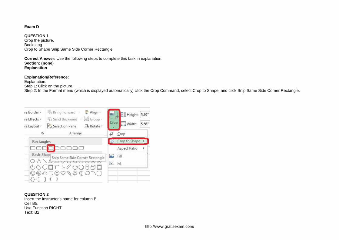
QUESTION 1Crop the picture.Books.jpgCrop to Shape Snip Same Side Corner Rectangle.
Correct Answer: Use the following steps to complete this task in explanation:Section: (none)Explanation
Explanation/Reference:Explanation:Step 1: Click on the picture.Step 2: In the Format menu (which is displayed automatically) click the Crop Command, select Crop to Shape, and click Snip Same Side Corner Rectangle.
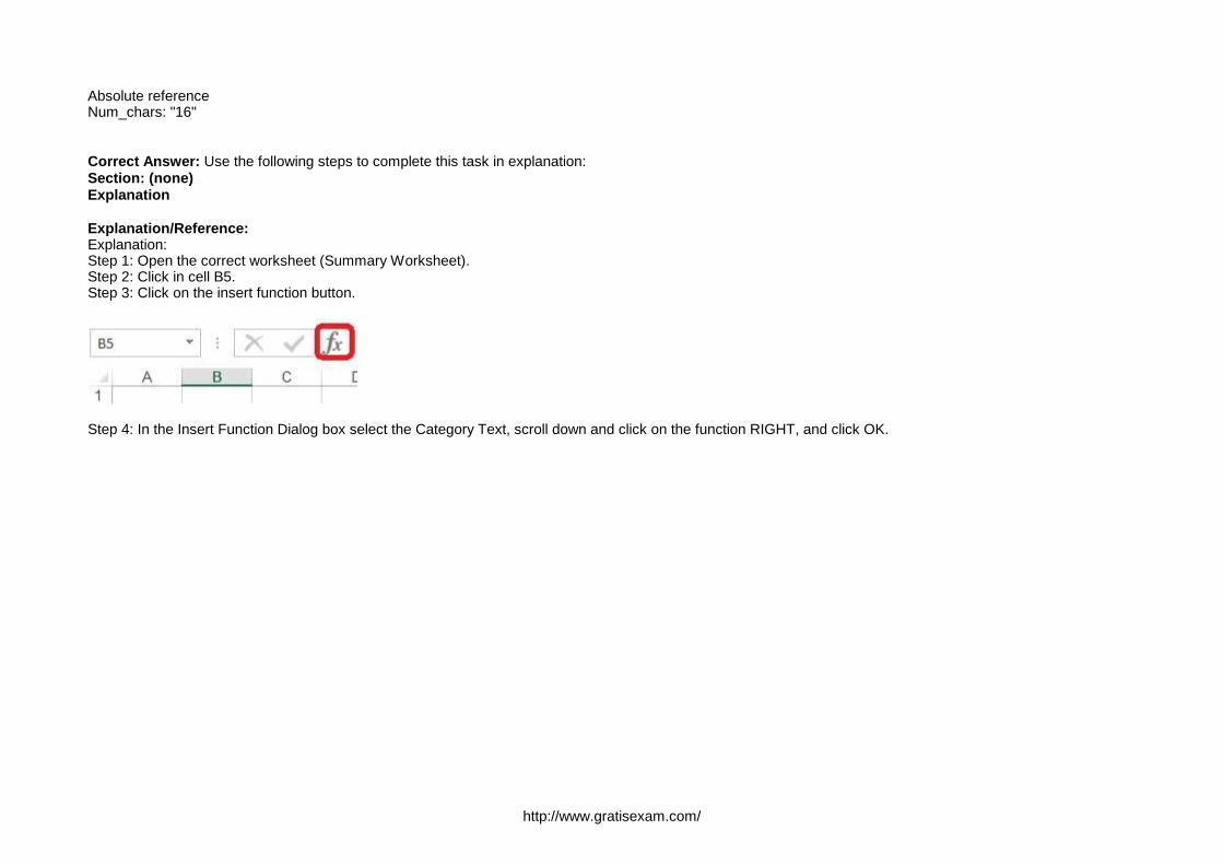
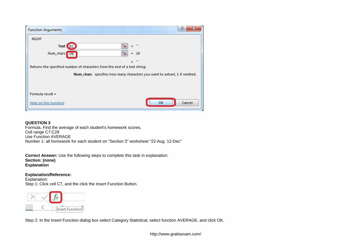
QUESTION 2Insert the instructor's name for column B.Cell B5.Use Function RIGHTText: B2
http://www.gratisexam.com/
Absolute referenceNum_chars: "16"
Correct Answer: Use the following steps to complete this task in explanation:Section: (none)Explanation
Explanation/Reference:Explanation:Step 1: Open the correct worksheet (Summary Worksheet).Step 2: Click in cell B5.Step 3: Click on the insert function button.
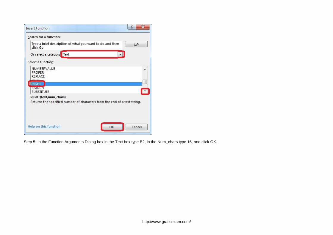
Step 4: In the Insert Function Dialog box select the Category Text, scroll down and click on the function RIGHT, and click OK.
http://www.gratisexam.com/
Step 5: In the Function Arguments Dialog box in the Text box type B2, in the Num_chars type 16, and click OK.
http://www.gratisexam.com/
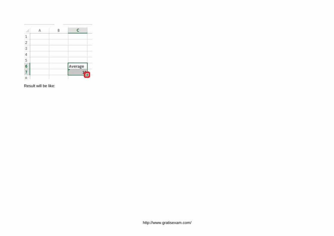
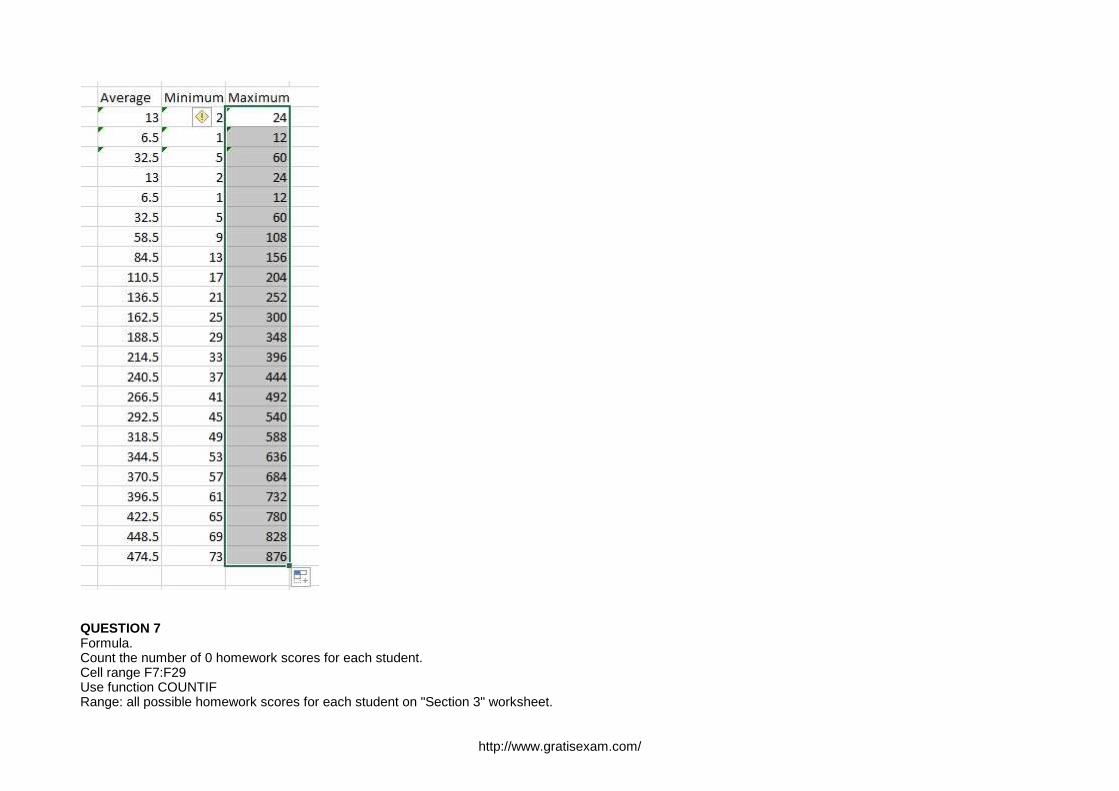
QUESTION 3Formula. Find the average of each student's homework scores.Cell range C7:C29Use Function AVERAGENumber 1: all homework for each student on "Section 3" worksheet "22-Aug 12-Dec"
Correct Answer: Use the following steps to complete this task in explanation:Section: (none)Explanation
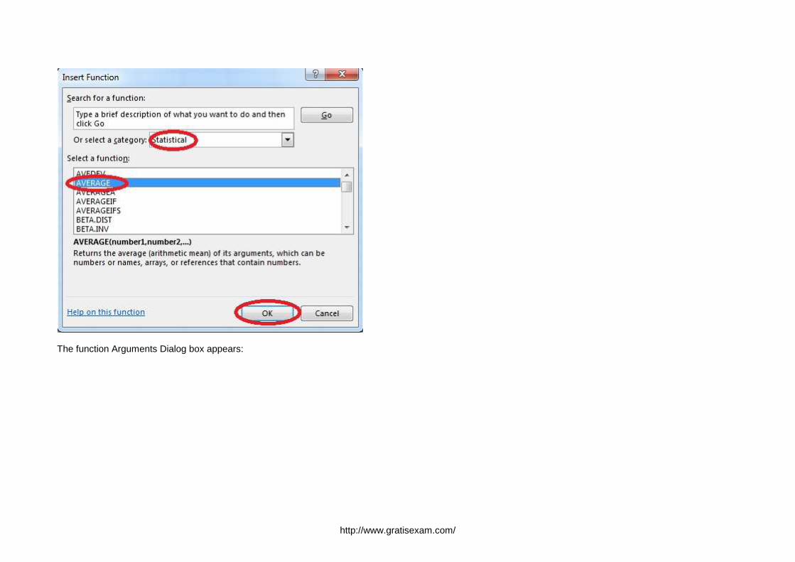
Explanation/Reference:Explanation:Step 1: Click cell C7, and the click the Insert Function Button.
Step 2: In the Insert Function dialog box select Category Statistical, select function AVERAGE, and click OK.
http://www.gratisexam.com/
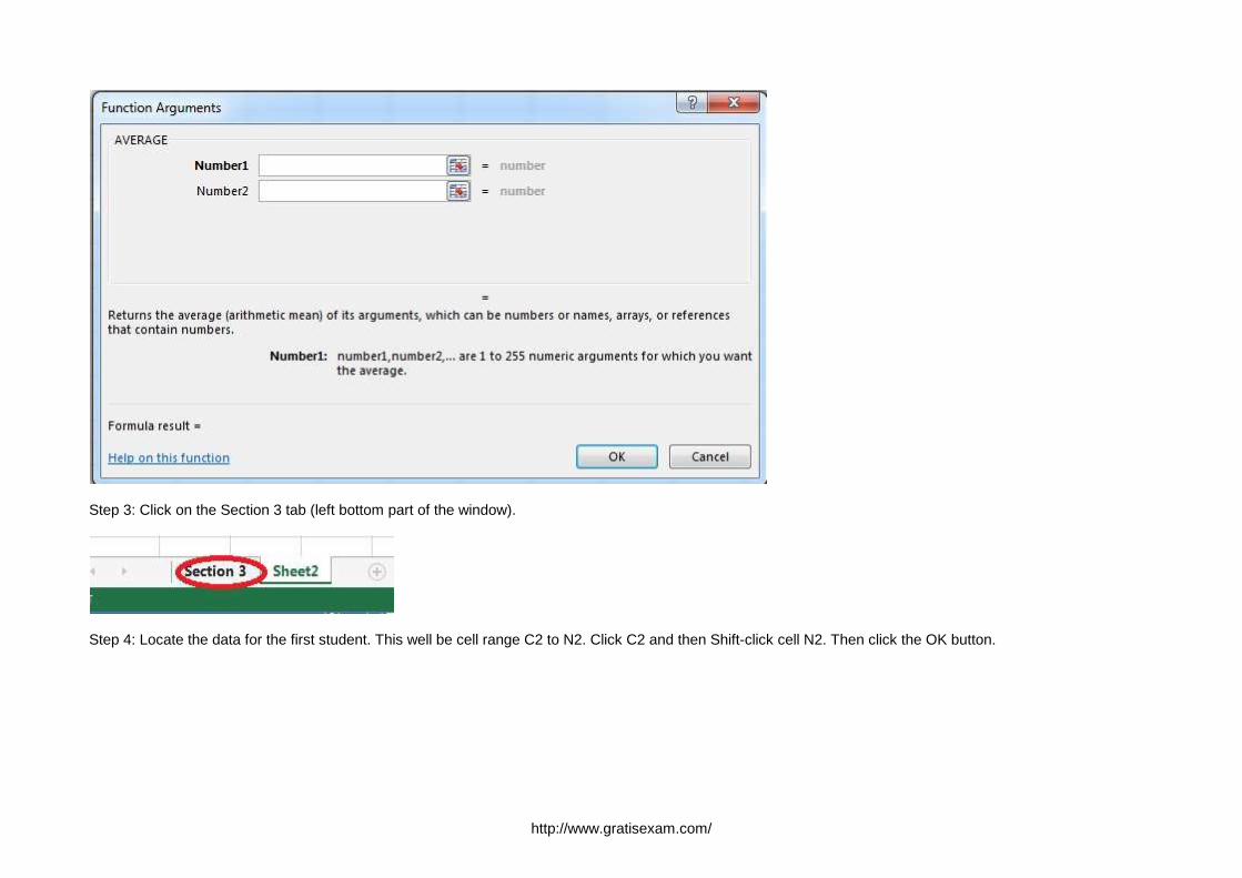
The function Arguments Dialog box appears:
http://www.gratisexam.com/
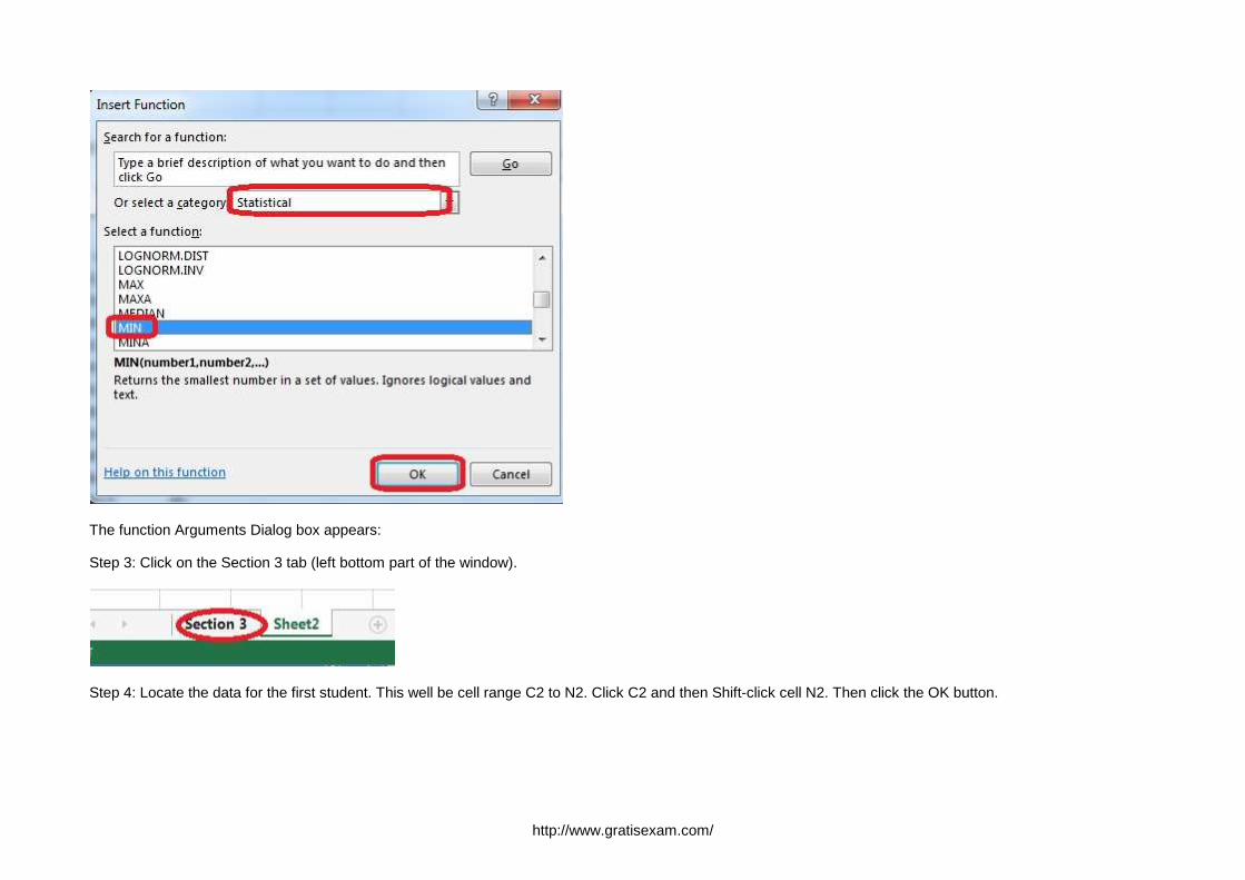
Step 3: Click on the Section 3 tab (left bottom part of the window).
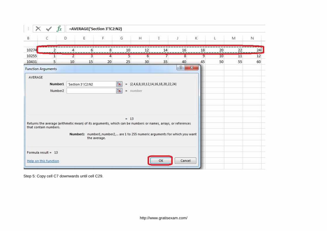
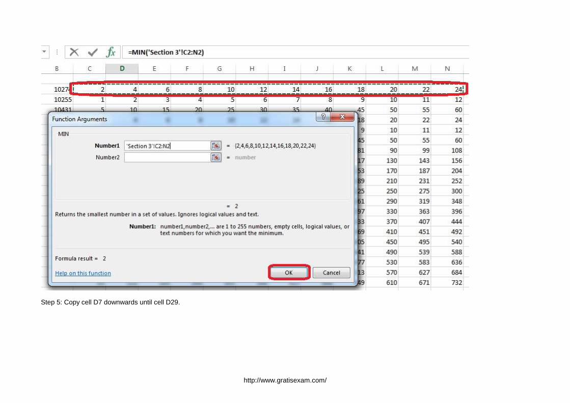
Step 4: Locate the data for the first student. This well be cell range C2 to N2. Click C2 and then Shift-click cell N2. Then click the OK button.
http://www.gratisexam.com/
Step 5: Copy cell C7 downwards until cell C29.
http://www.gratisexam.com/
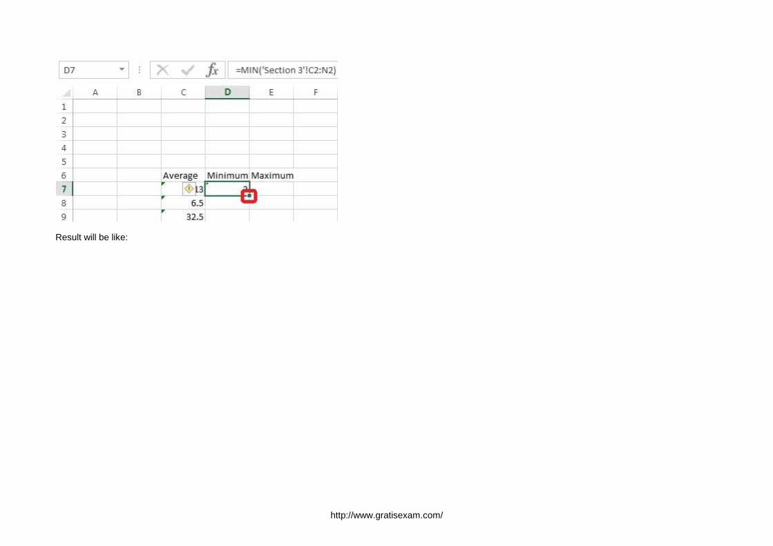
Result will be like:
http://www.gratisexam.com/
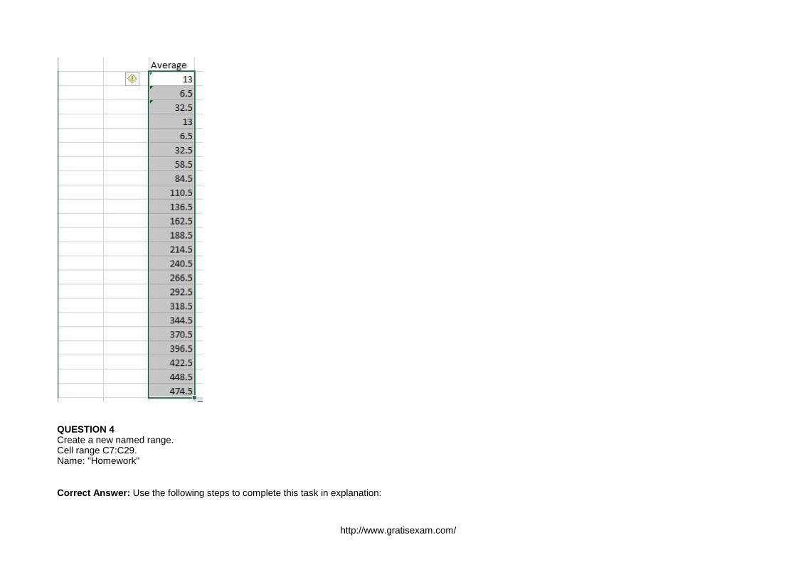
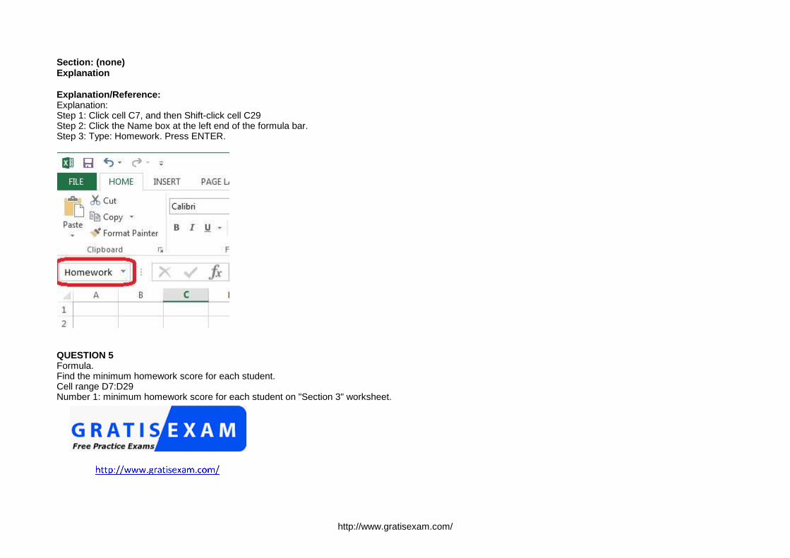
QUESTION 4Create a new named range.Cell range C7:C29.Name: "Homework"
Correct Answer: Use the following steps to complete this task in explanation:
http://www.gratisexam.com/
Section: (none)Explanation
Explanation/Reference:Explanation:Step 1: Click cell C7, and then Shift-click cell C29Step 2: Click the Name box at the left end of the formula bar. Step 3: Type: Homework. Press ENTER.
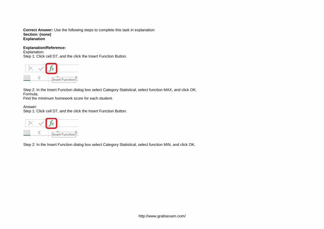
QUESTION 5Formula.Find the minimum homework score for each student.Cell range D7:D29Number 1: minimum homework score for each student on "Section 3" worksheet.
http://www.gratisexam.com/
Correct Answer: Use the following steps to complete this task in explanation:Section: (none)Explanation
Explanation/Reference:Explanation:Step 1: Click cell D7, and the click the Insert Function Button.
Step 2: In the Insert Function dialog box select Category Statistical, select function MAX, and click OK.Formula.Find the minimum homework score for each student.
Answer: Step 1: Click cell D7, and the click the Insert Function Button.
Step 2: In the Insert Function dialog box select Category Statistical, select function MIN, and click OK.
http://www.gratisexam.com/
The function Arguments Dialog box appears:
Step 3: Click on the Section 3 tab (left bottom part of the window).
Step 4: Locate the data for the first student. This well be cell range C2 to N2. Click C2 and then Shift-click cell N2. Then click the OK button.
http://www.gratisexam.com/
Step 5: Copy cell D7 downwards until cell D29.
http://www.gratisexam.com/
Result will be like:
http://www.gratisexam.com/
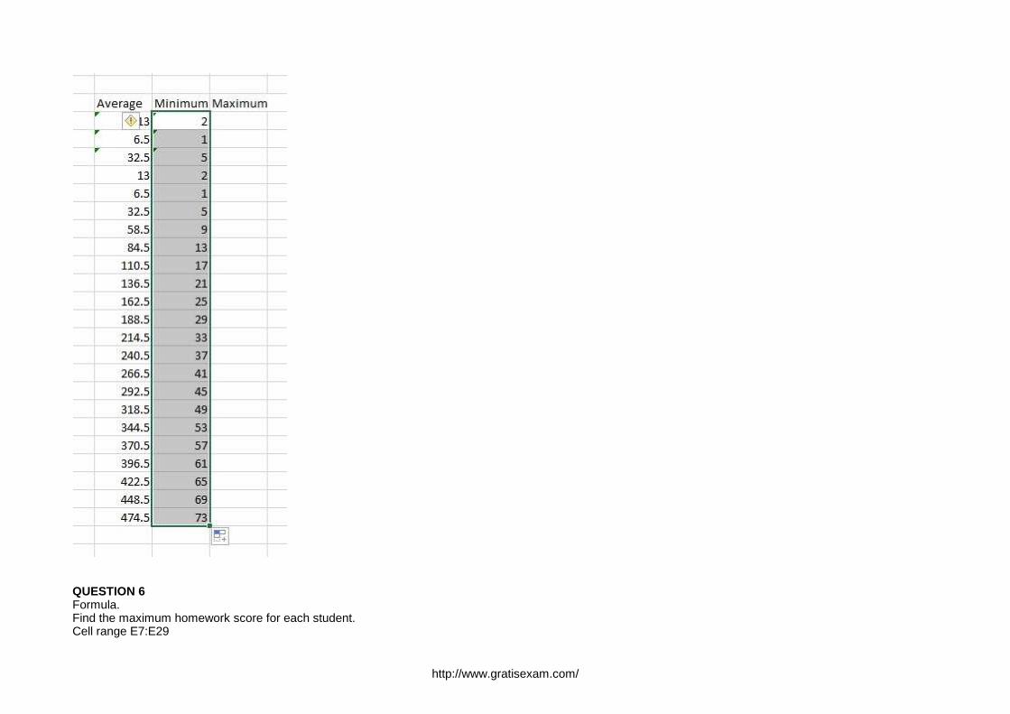
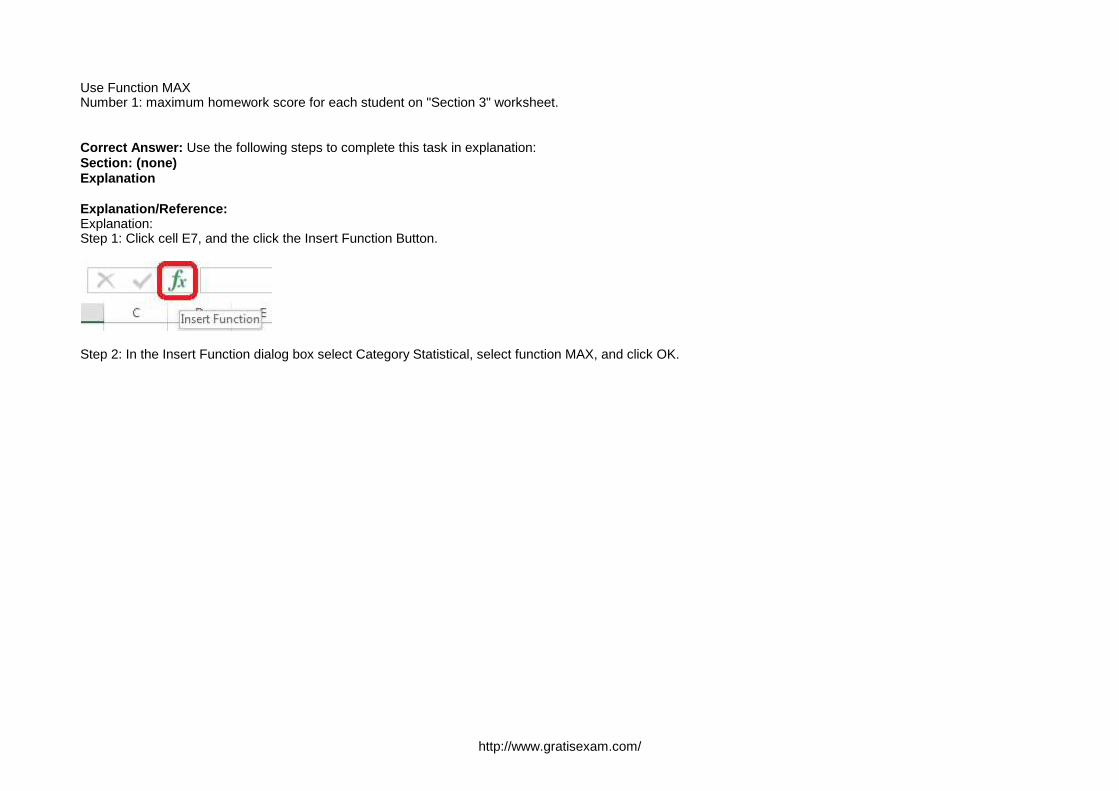
QUESTION 6Formula.Find the maximum homework score for each student.Cell range E7:E29
http://www.gratisexam.com/
Use Function MAXNumber 1: maximum homework score for each student on "Section 3" worksheet.
Correct Answer: Use the following steps to complete this task in explanation:Section: (none)Explanation
Explanation/Reference:Explanation:Step 1: Click cell E7, and the click the Insert Function Button.
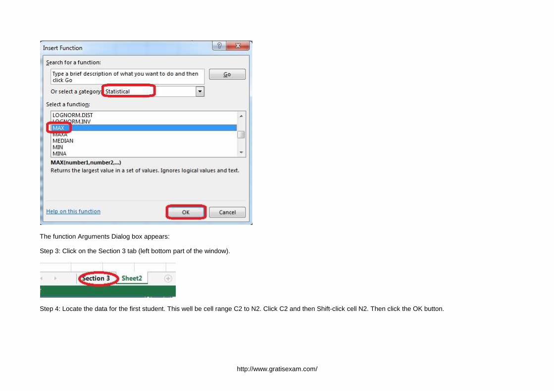
Step 2: In the Insert Function dialog box select Category Statistical, select function MAX, and click OK.
http://www.gratisexam.com/
The function Arguments Dialog box appears:
Step 3: Click on the Section 3 tab (left bottom part of the window).
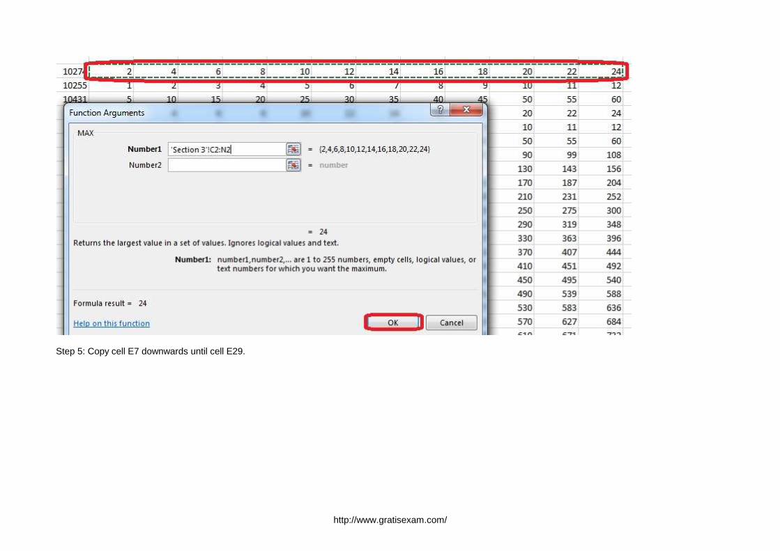
Step 4: Locate the data for the first student. This well be cell range C2 to N2. Click C2 and then Shift-click cell N2. Then click the OK button.
http://www.gratisexam.com/
Step 5: Copy cell E7 downwards until cell E29.
http://www.gratisexam.com/
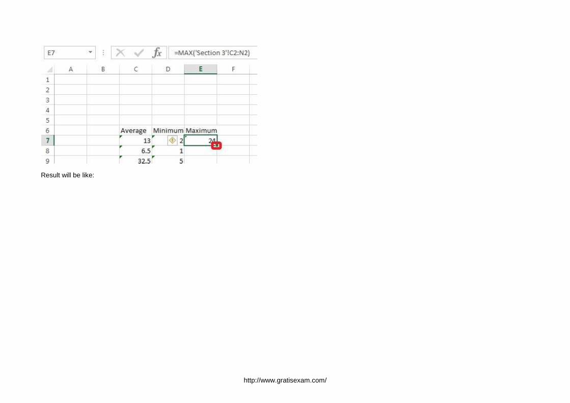
Result will be like:
http://www.gratisexam.com/
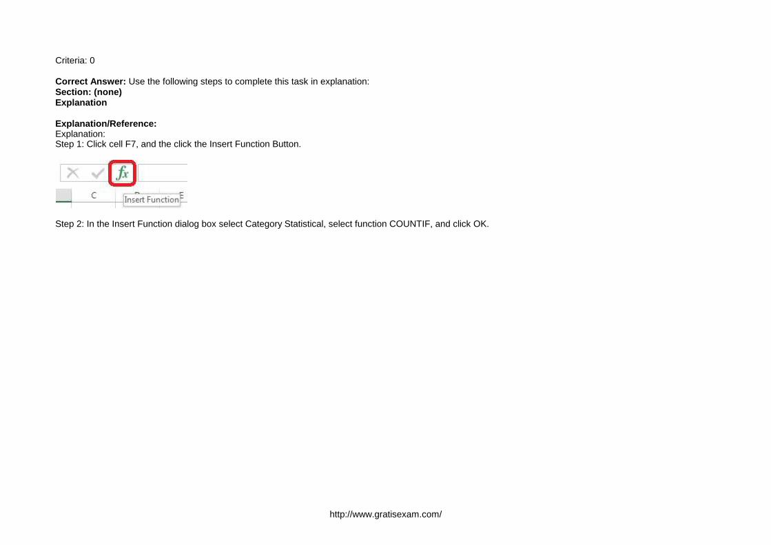
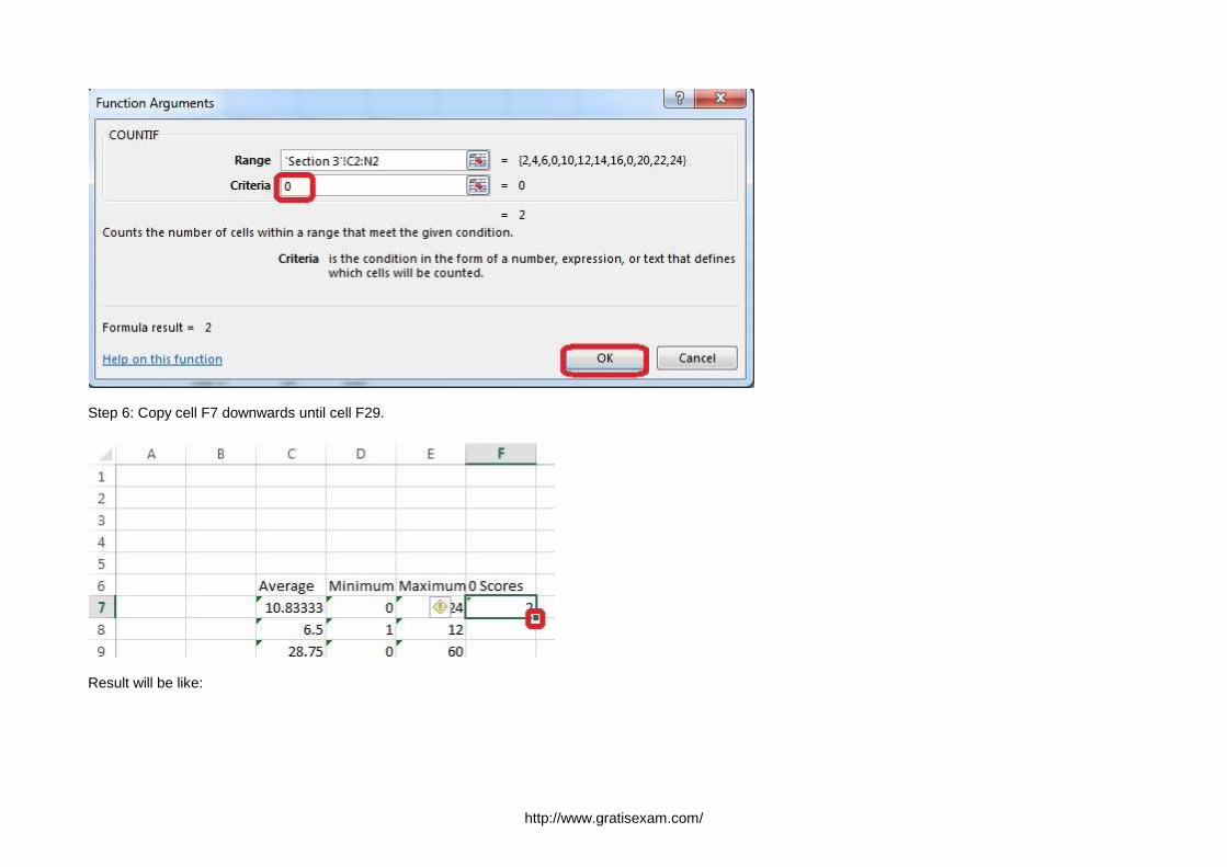
QUESTION 7Formula.Count the number of 0 homework scores for each student.Cell range F7:F29Use function COUNTIFRange: all possible homework scores for each student on "Section 3" worksheet.
http://www.gratisexam.com/
Criteria: 0
Correct Answer: Use the following steps to complete this task in explanation:Section: (none)Explanation
Explanation/Reference:Explanation:Step 1: Click cell F7, and the click the Insert Function Button.
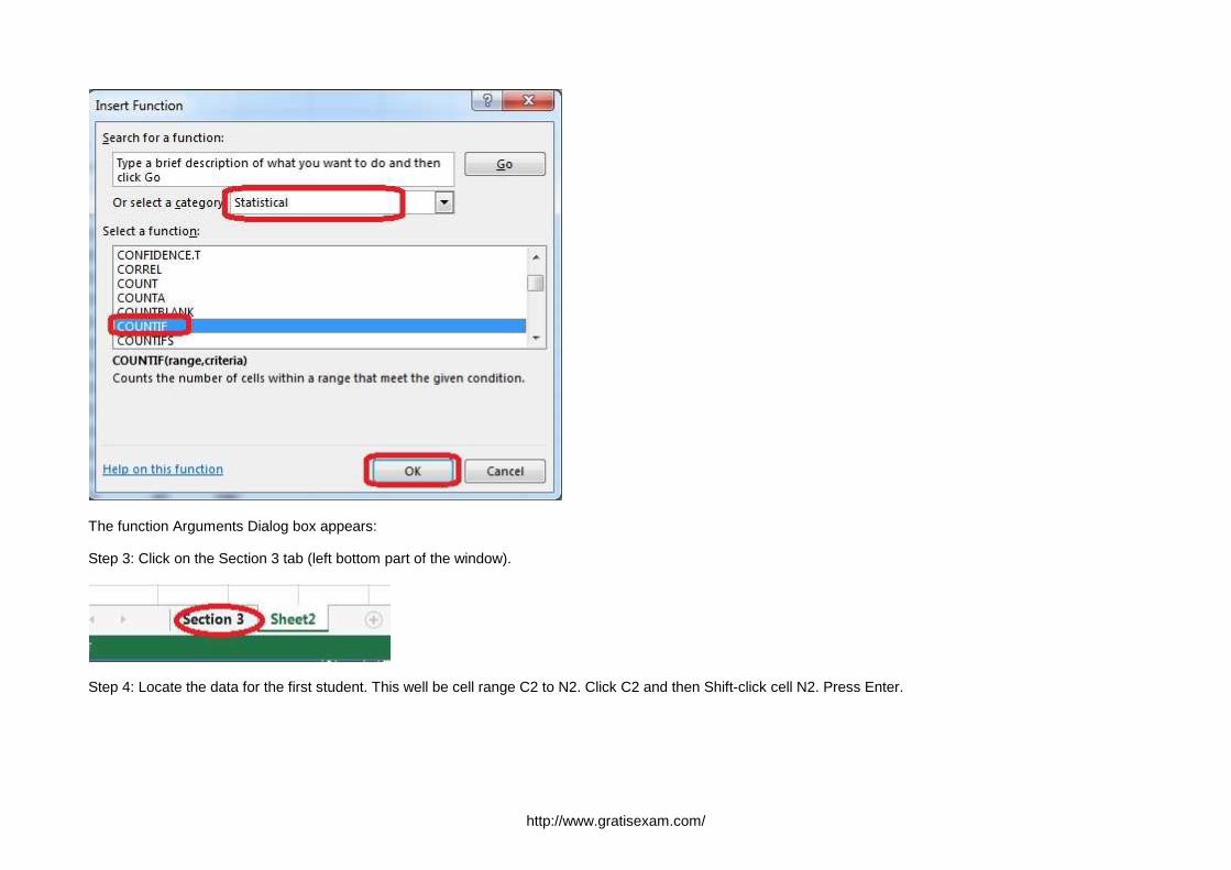
Step 2: In the Insert Function dialog box select Category Statistical, select function COUNTIF, and click OK.
http://www.gratisexam.com/
The function Arguments Dialog box appears:
Step 3: Click on the Section 3 tab (left bottom part of the window).
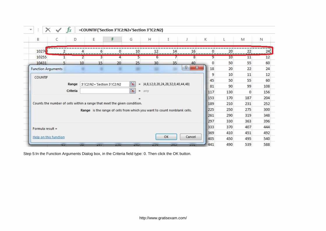
Step 4: Locate the data for the first student. This well be cell range C2 to N2. Click C2 and then Shift-click cell N2. Press Enter.
http://www.gratisexam.com/
Step 5:In the Function Arguments Dialog box, in the Criteria field type: 0. Then click the OK button.
http://www.gratisexam.com/
Step 6: Copy cell F7 downwards until cell F29.
Result will be like:
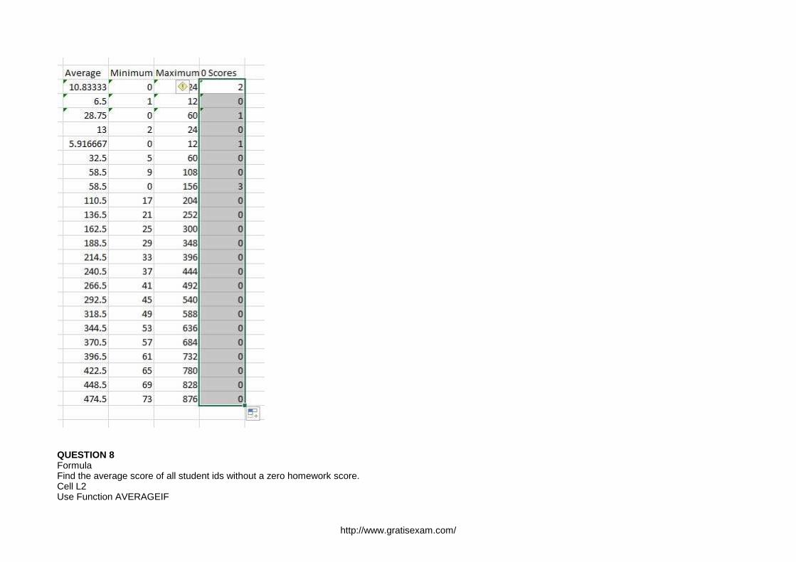
http://www.gratisexam.com/
QUESTION 8FormulaFind the average score of all student ids without a zero homework score.Cell L2Use Function AVERAGEIF
http://www.gratisexam.com/
Range F7:F29Criteria: "0"Average_range: "Homework"
Correct Answer: Use the following steps to complete this task in explanation:Section: (none)Explanation
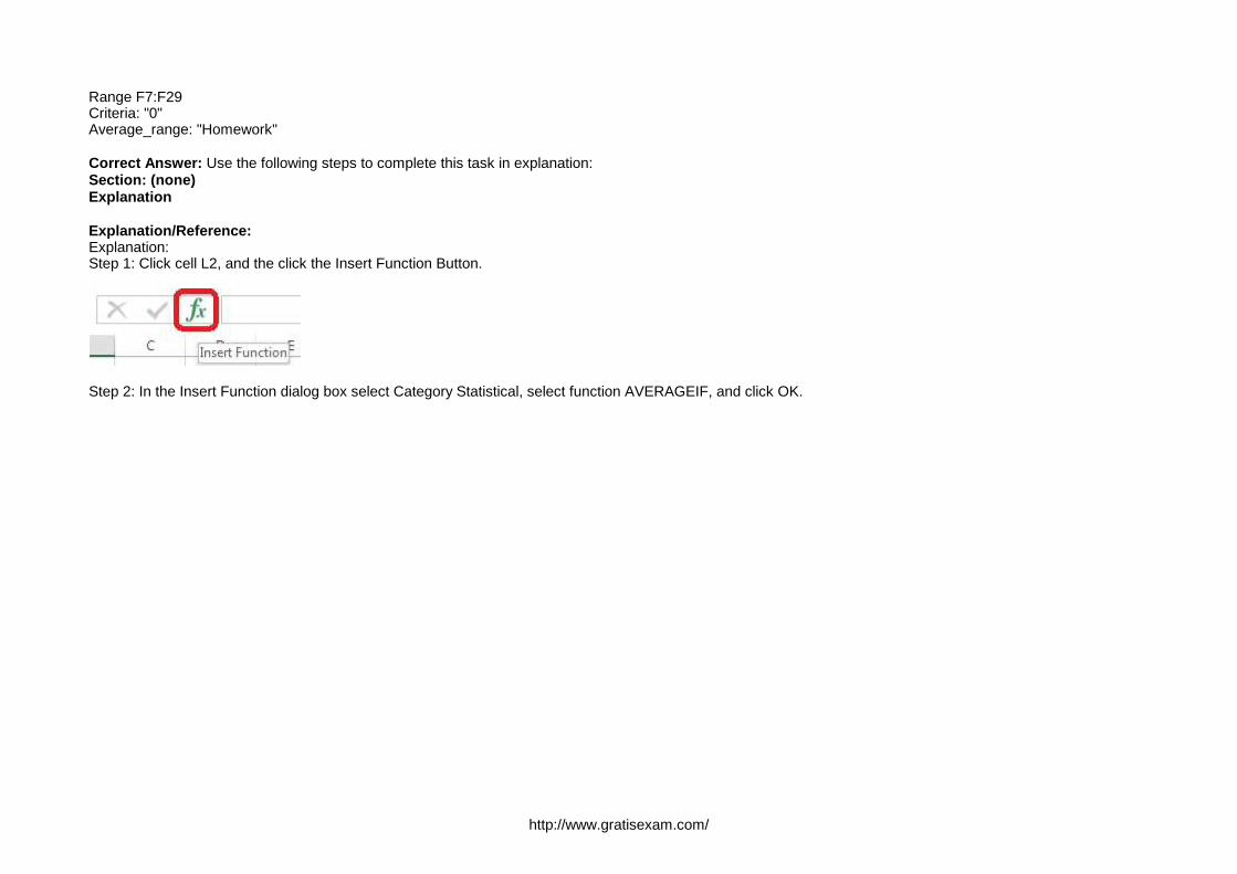
Explanation/Reference:Explanation:Step 1: Click cell L2, and the click the Insert Function Button.
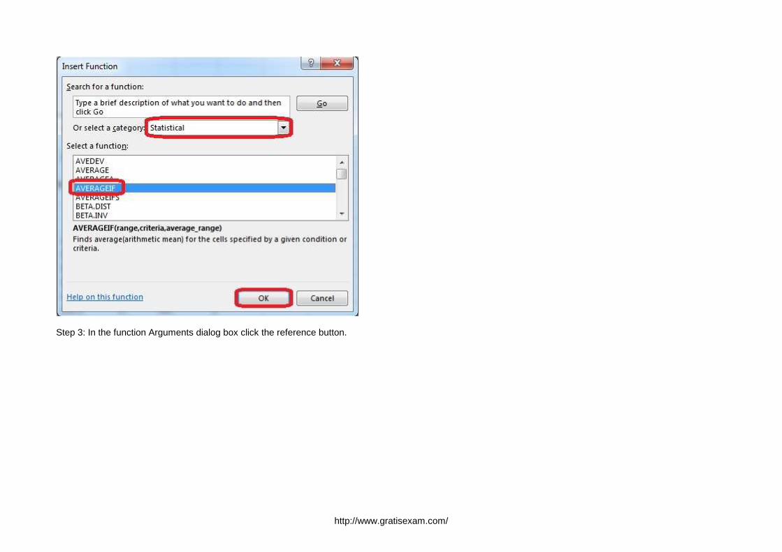
Step 2: In the Insert Function dialog box select Category Statistical, select function AVERAGEIF, and click OK.
http://www.gratisexam.com/
Step 3: In the function Arguments dialog box click the reference button.
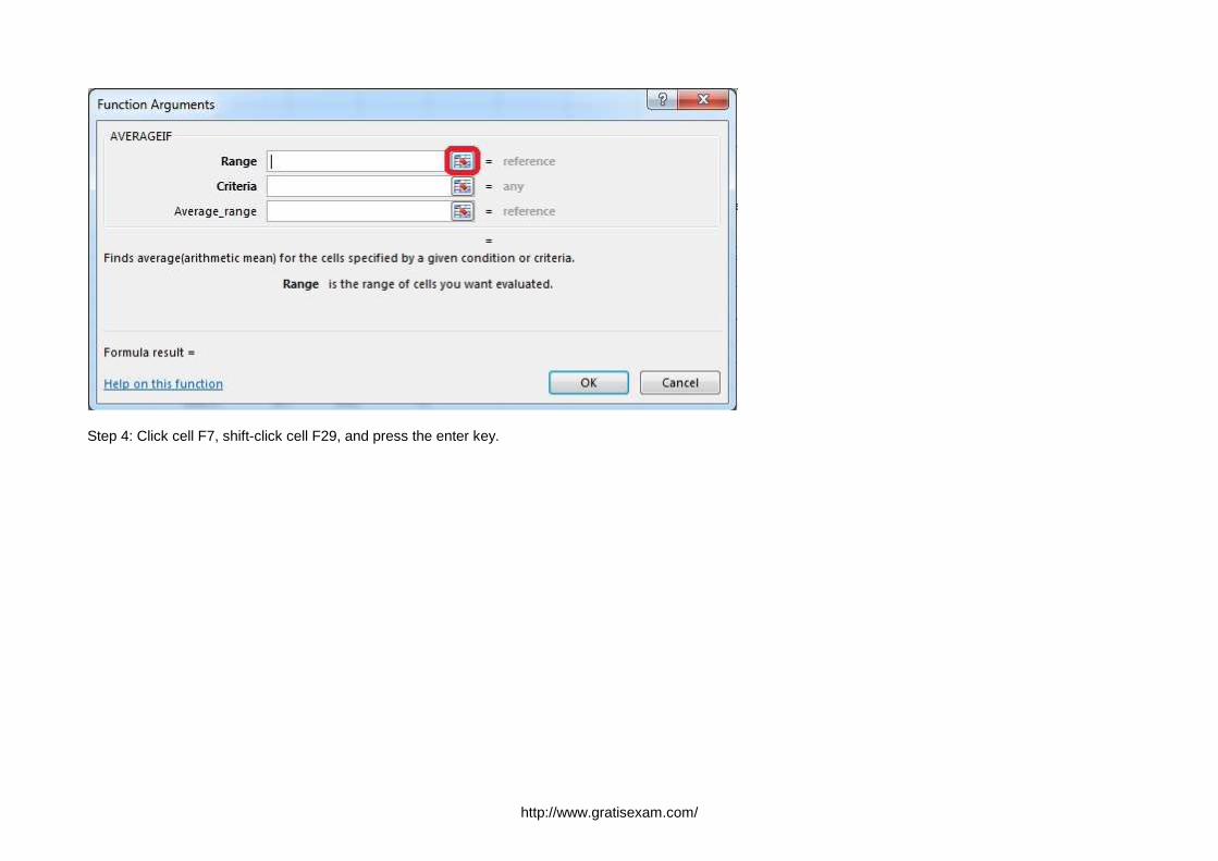
http://www.gratisexam.com/
Step 4: Click cell F7, shift-click cell F29, and press the enter key.
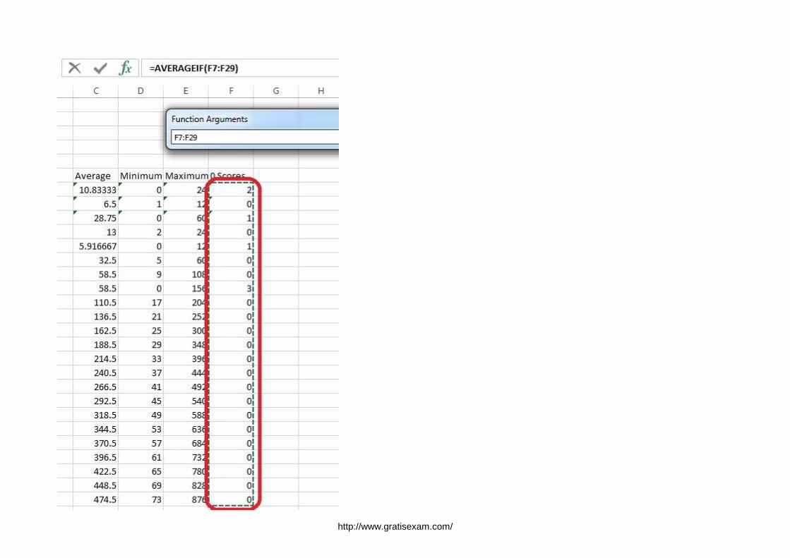
http://www.gratisexam.com/
http://www.gratisexam.com/
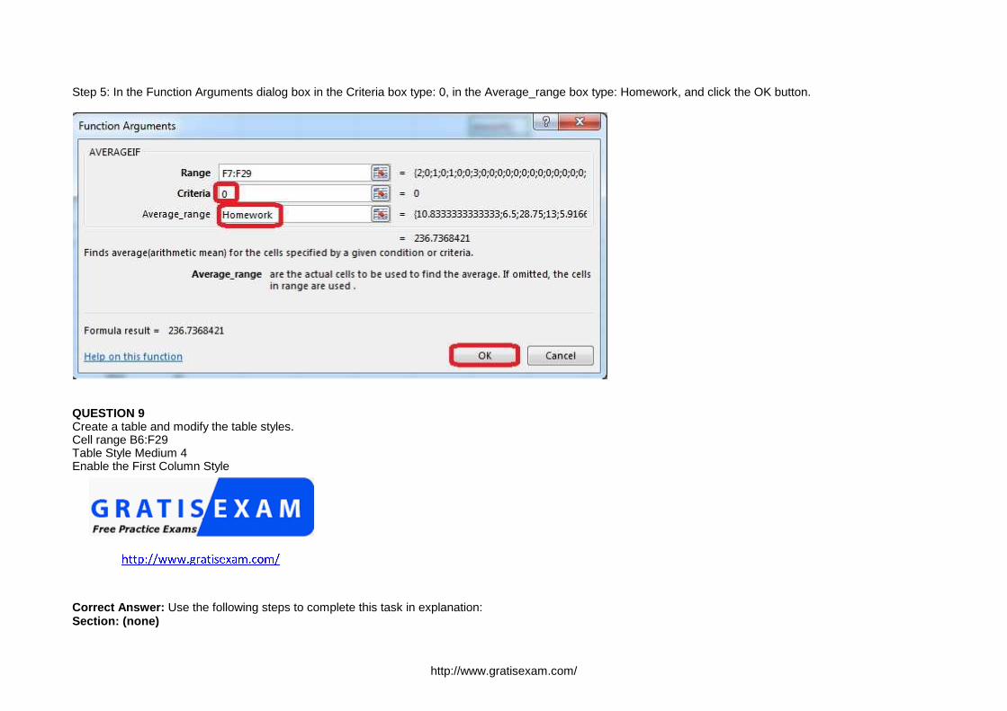
Step 5: In the Function Arguments dialog box in the Criteria box type: 0, in the Average_range box type: Homework, and click the OK button.
QUESTION 9Create a table and modify the table styles.Cell range B6:F29Table Style Medium 4Enable the First Column Style
Correct Answer: Use the following steps to complete this task in explanation:Section: (none)
http://www.gratisexam.com/
Explanation
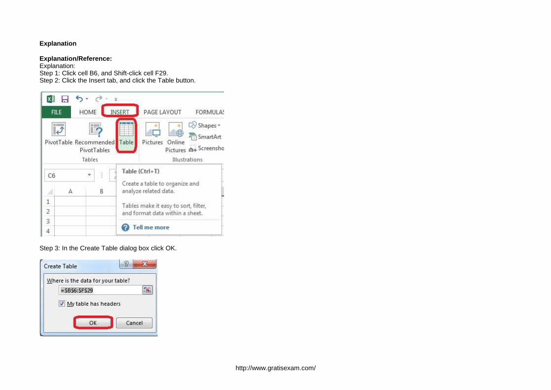
Explanation/Reference:Explanation:Step 1: Click cell B6, and Shift-click cell F29.Step 2: Click the Insert tab, and click the Table button.
Step 3: In the Create Table dialog box click OK.
http://www.gratisexam.com/
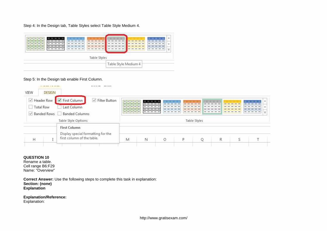
Step 4: In the Design tab, Table Styles select Table Style Medium 4.
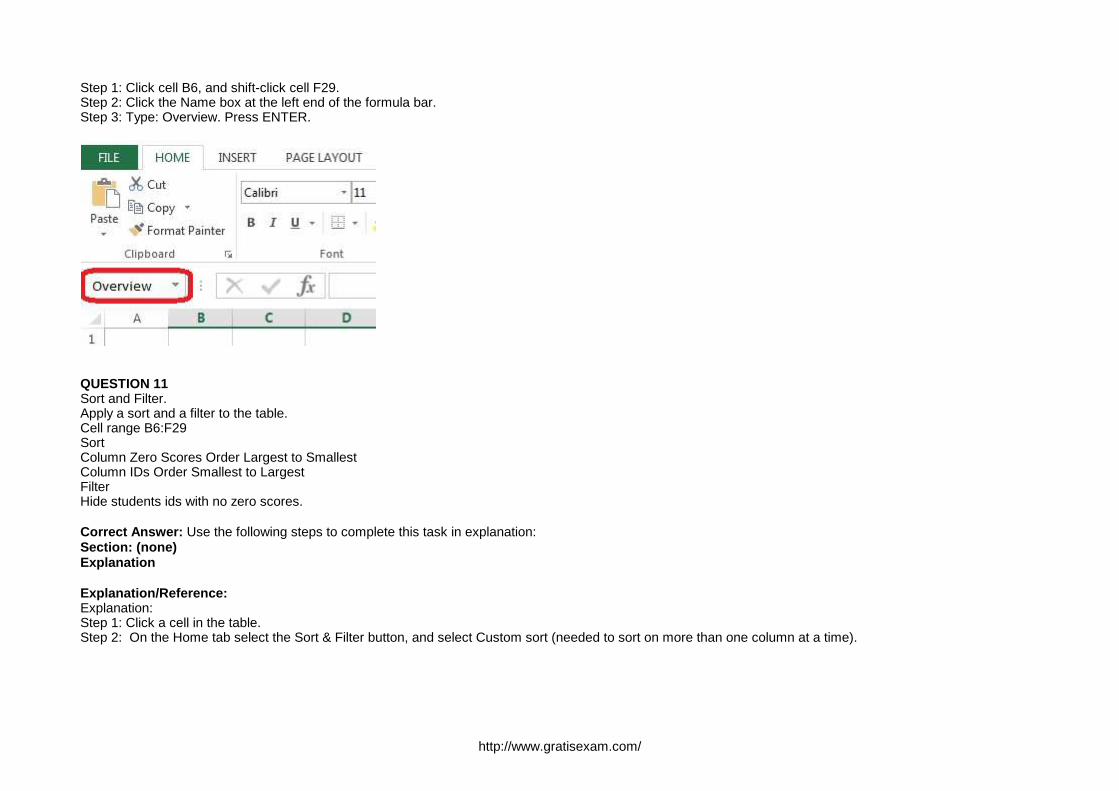
Step 5: In the Design tab enable First Column.
QUESTION 10Rename a table.Cell range B6:F29Name: "Overview"
Correct Answer: Use the following steps to complete this task in explanation:Section: (none)Explanation
Explanation/Reference:Explanation:
http://www.gratisexam.com/
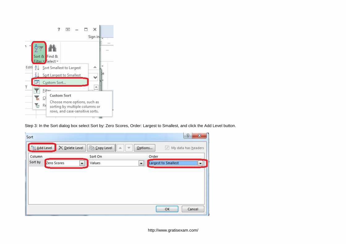
Step 1: Click cell B6, and shift-click cell F29.Step 2: Click the Name box at the left end of the formula bar. Step 3: Type: Overview. Press ENTER.
QUESTION 11Sort and Filter.Apply a sort and a filter to the table.Cell range B6:F29SortColumn Zero Scores Order Largest to SmallestColumn IDs Order Smallest to LargestFilterHide students ids with no zero scores.
Correct Answer: Use the following steps to complete this task in explanation:Section: (none)Explanation
Explanation/Reference:Explanation:Step 1: Click a cell in the table.Step 2: On the Home tab select the Sort & Filter button, and select Custom sort (needed to sort on more than one column at a time).
http://www.gratisexam.com/
Step 3: In the Sort dialog box select Sort by: Zero Scores, Order: Largest to Smallest, and click the Add Level button.
http://www.gratisexam.com/
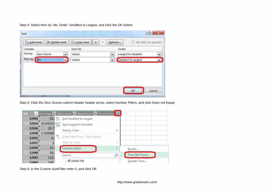
Step 4: Select then by: Ids, Order: Smallest to Largest, and click the OK button.
Step 5: Click the Zero Scores column header header arrow, select Number Filters, and click Does not Equal.
Step 6: In the Custom AutoFilter enter 0, and click OK

http://www.gratisexam.com/
The result will look like:
http://www.gratisexam.com/
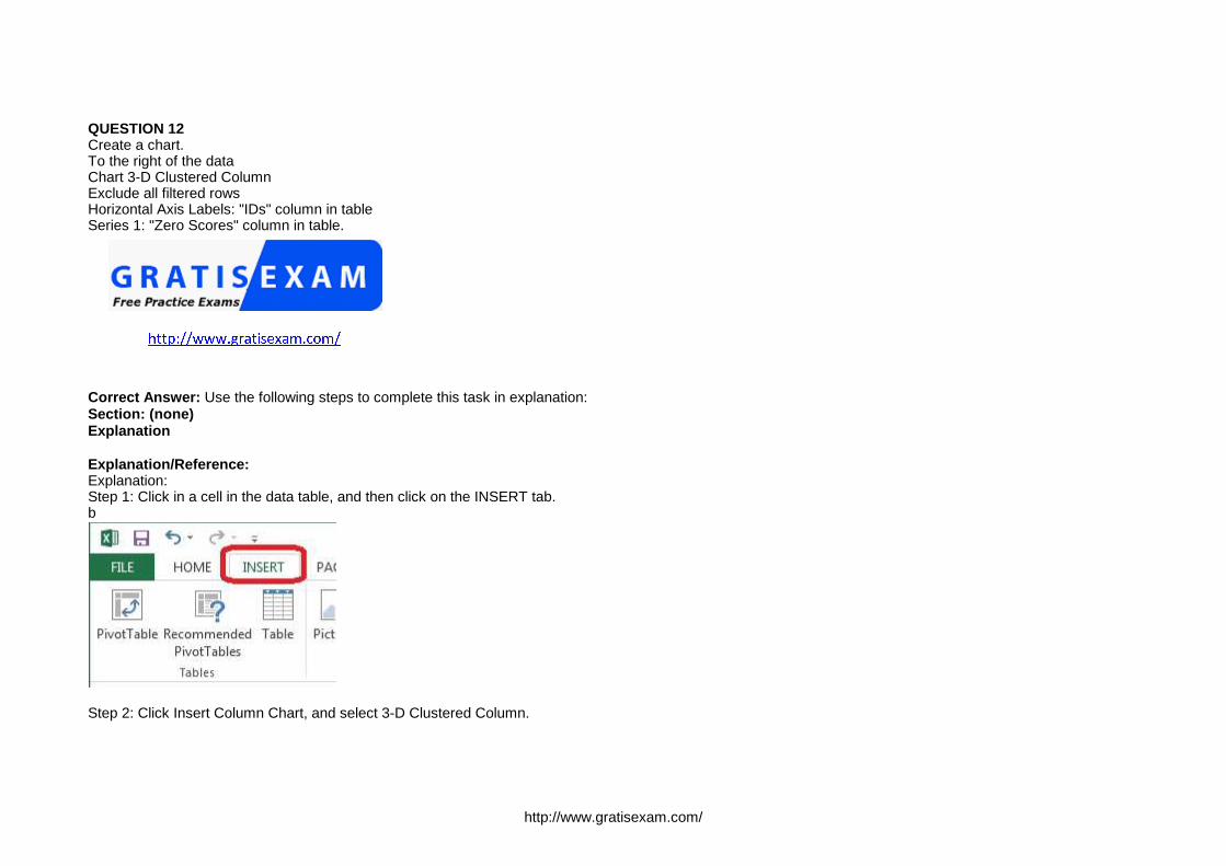
QUESTION 12Create a chart.To the right of the dataChart 3-D Clustered ColumnExclude all filtered rowsHorizontal Axis Labels: "IDs" column in tableSeries 1: "Zero Scores" column in table.
Correct Answer: Use the following steps to complete this task in explanation:Section: (none)Explanation
Explanation/Reference:Explanation:Step 1: Click in a cell in the data table, and then click on the INSERT tab.b
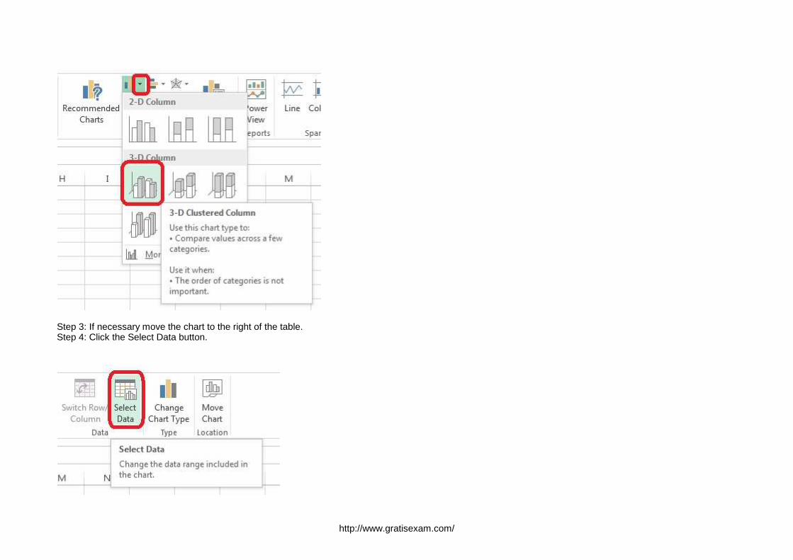
Step 2: Click Insert Column Chart, and select 3-D Clustered Column.
http://www.gratisexam.com/
Step 3: If necessary move the chart to the right of the table.Step 4: Click the Select Data button.
http://www.gratisexam.com/
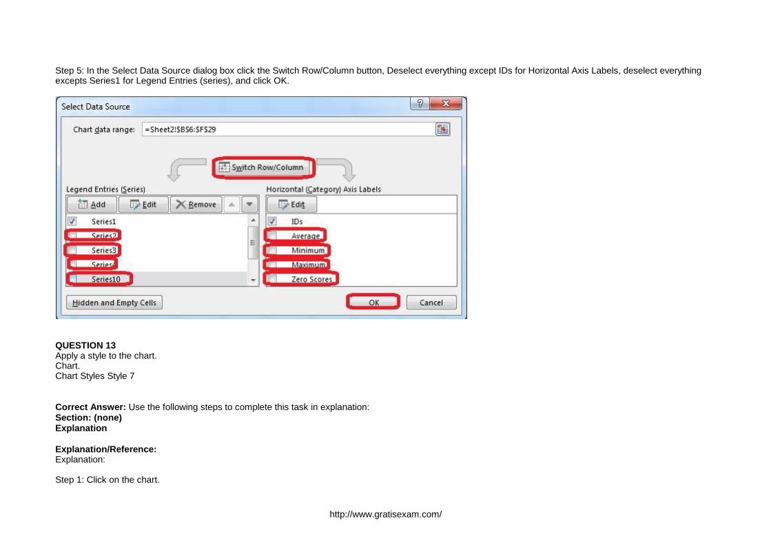
Step 5: In the Select Data Source dialog box click the Switch Row/Column button, Deselect everything except IDs for Horizontal Axis Labels, deselect everythingexcepts Series1 for Legend Entries (series), and click OK.
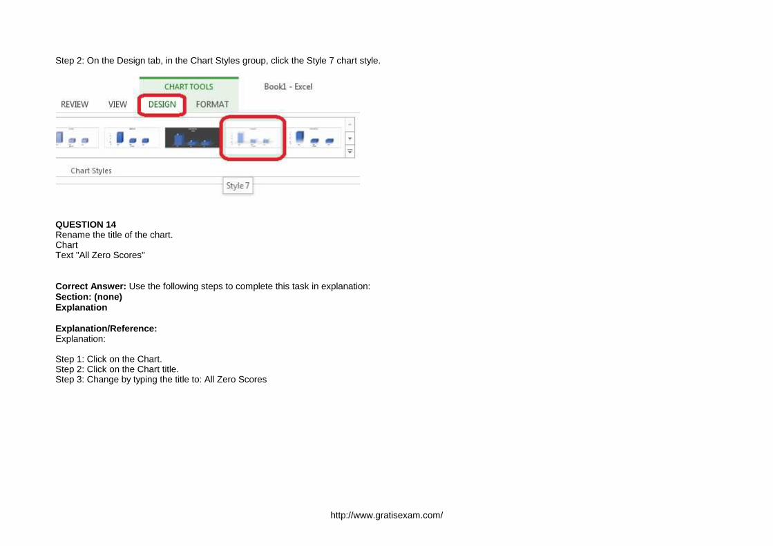
QUESTION 13Apply a style to the chart.Chart.Chart Styles Style 7
Correct Answer: Use the following steps to complete this task in explanation:Section: (none)Explanation
Explanation/Reference:Explanation:
Step 1: Click on the chart.
http://www.gratisexam.com/
Step 2: On the Design tab, in the Chart Styles group, click the Style 7 chart style.
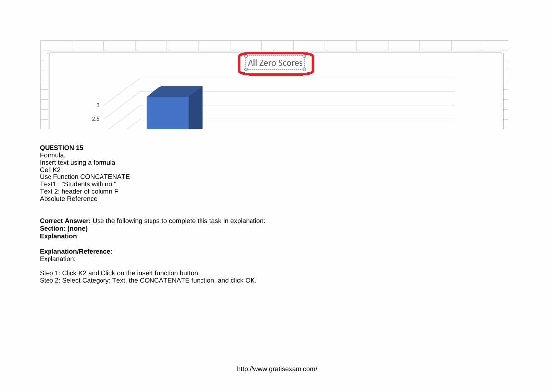
QUESTION 14Rename the title of the chart.ChartText "All Zero Scores"
Correct Answer: Use the following steps to complete this task in explanation:Section: (none)Explanation
Explanation/Reference:Explanation:
Step 1: Click on the Chart.Step 2: Click on the Chart title.Step 3: Change by typing the title to: All Zero Scores
http://www.gratisexam.com/
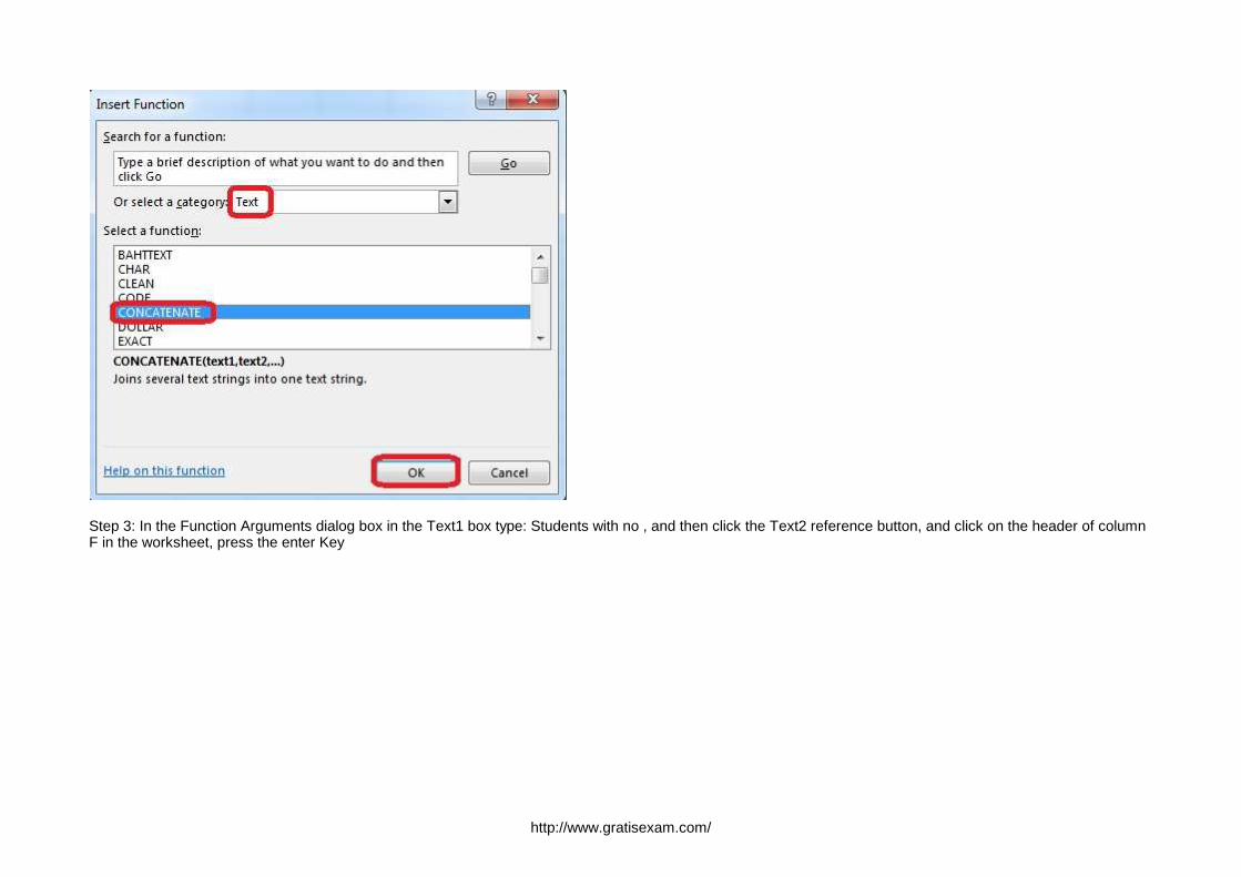
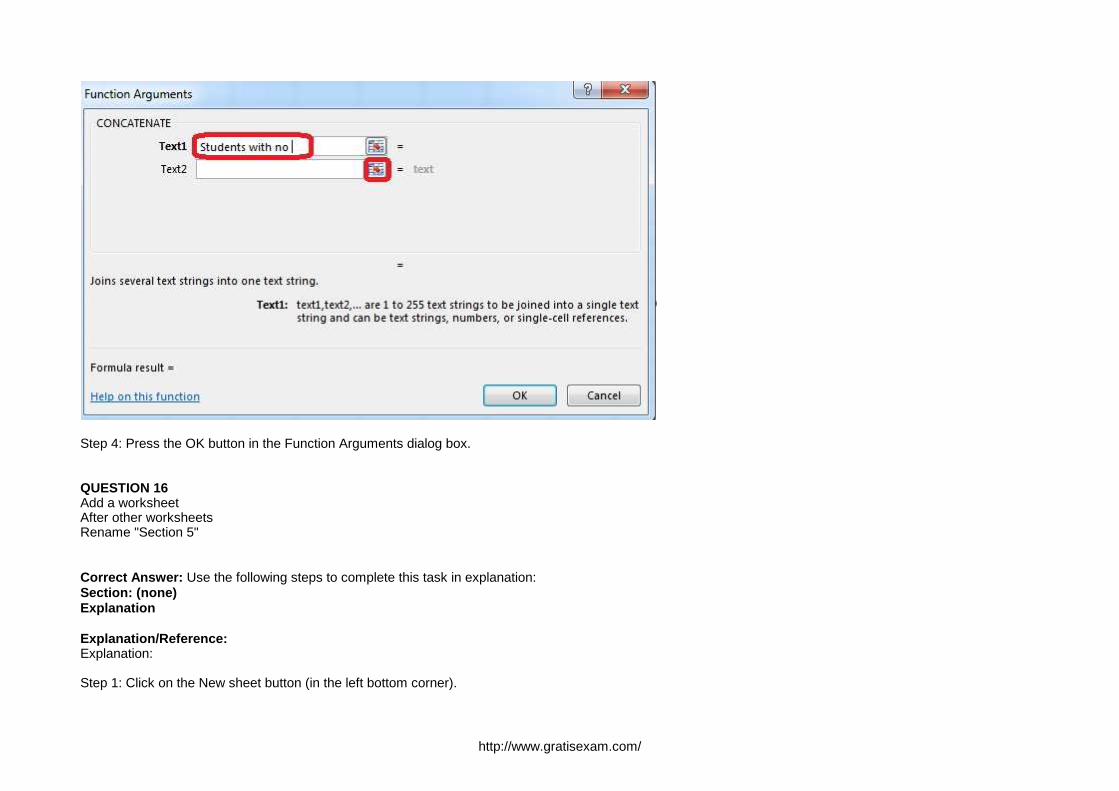
QUESTION 15Formula.Insert text using a formulaCell K2Use Function CONCATENATEText1 : "Students with no "Text 2: header of column FAbsolute Reference
Correct Answer: Use the following steps to complete this task in explanation:Section: (none)Explanation
Explanation/Reference:Explanation:
Step 1: Click K2 and Click on the insert function button.Step 2: Select Category: Text, the CONCATENATE function, and click OK.
http://www.gratisexam.com/
Step 3: In the Function Arguments dialog box in the Text1 box type: Students with no , and then click the Text2 reference button, and click on the header of columnF in the worksheet, press the enter Key
http://www.gratisexam.com/
Step 4: Press the OK button in the Function Arguments dialog box.
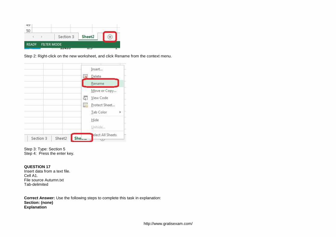
QUESTION 16Add a worksheetAfter other worksheetsRename "Section 5"
Correct Answer: Use the following steps to complete this task in explanation:Section: (none)Explanation
Explanation/Reference:Explanation:
Step 1: Click on the New sheet button (in the left bottom corner).
http://www.gratisexam.com/
Step 2: Right-click on the new worksheet, and click Rename from the context menu.
Step 3: Type: Section 5Step 4: Press the enter key.
QUESTION 17Insert data from a text file.Cell A1.File source Autumn.txtTab-delimited
Correct Answer: Use the following steps to complete this task in explanation:Section: (none)Explanation
http://www.gratisexam.com/
Explanation/Reference:Explanation:
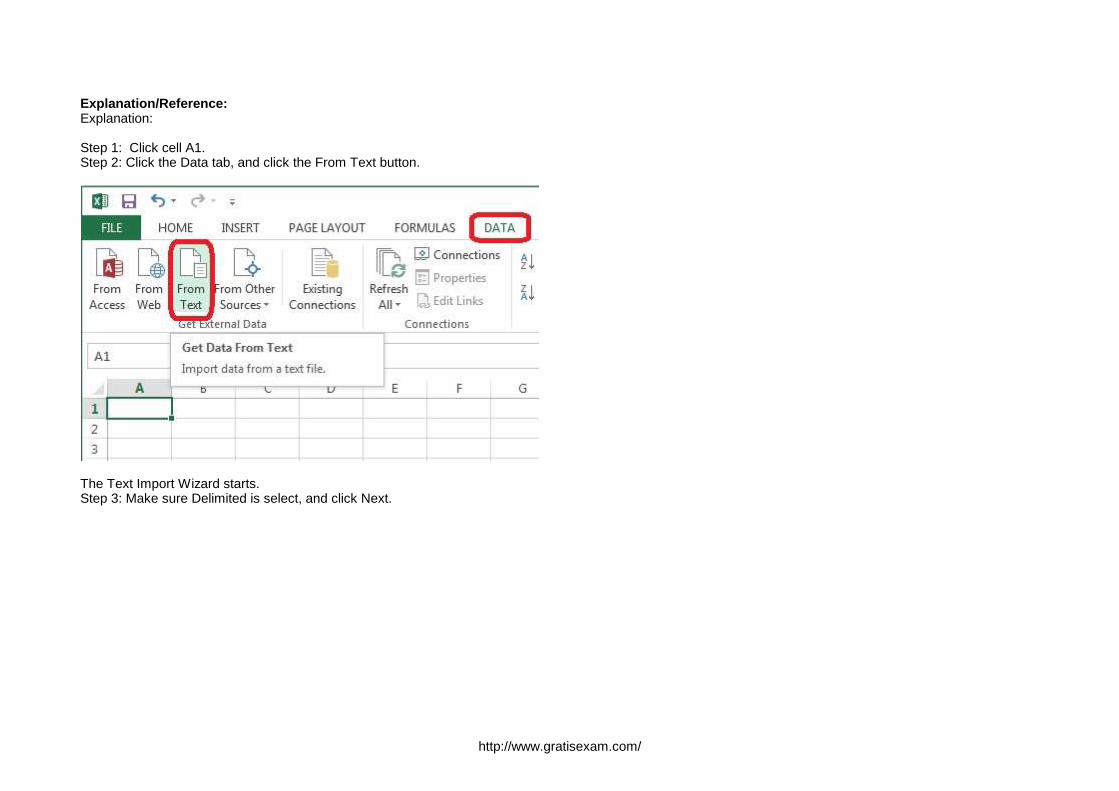
Step 1: Click cell A1.Step 2: Click the Data tab, and click the From Text button.
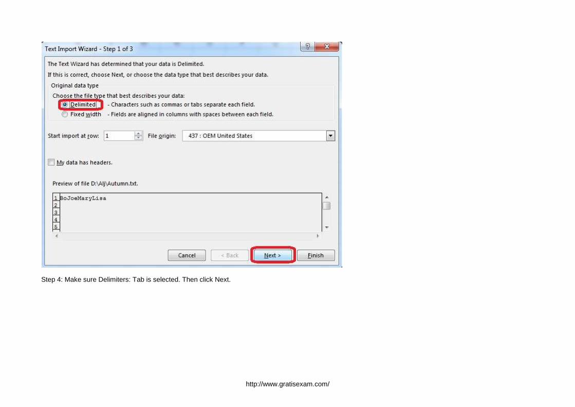
The Text Import Wizard starts.Step 3: Make sure Delimited is select, and click Next.
http://www.gratisexam.com/
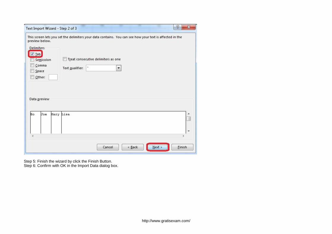
Step 4: Make sure Delimiters: Tab is selected. Then click Next.
http://www.gratisexam.com/
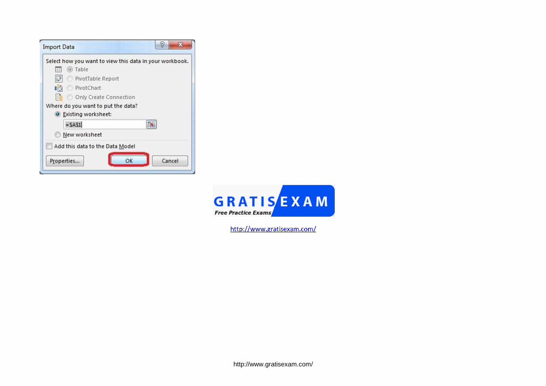
Step 5: Finish the wizard by click the Finish Button.Step 6: Confirm with OK in the Import Data dialog box.
http://www.gratisexam.com/