i

© Copyright 2016

John Hackney

ii

Essays on Personal Bankruptcy Law and Small Business Financing

John Hackney

A dissertation

submitted in partial fulfillment of the

requirements for the degree of

Doctor of Philosophy

University of Washington

2016

Reading Committee:

Ran Duchin, Chair

Edward Rice

Jonathan Karpoff

Program Authorized to Offer Degree:

Foster School of Business

iii

iv

University of Washington

Abstract

Essays on Personal Bankruptcy Law and Small Business Financing

John Hackney

Chair of the Supervisory Committee:

Associate Professor Ran Duchin

Department of Finance and Business Economics

In the first chapter of my dissertation I ask whether and how debtor protection affects

aggregate small business credit quantity. Using comprehensive data on the number and amount

of small business loans granted by commercial banks, and employing a robust difference-in-

difference empirical design utilizing staggered shocks to personal bankruptcy exemptions, I find

that increases in debtor protection increase the equilibrium quantity of small business credit in

local regions. This finding is statistically significant and robust, despite competing demand and

supply effects. I find that an average change in the homestead exemption results in a 1.1%

increase in the number of small business loans in a local area (census tract), and a 2.5% increase

in the total volume. The increase in quantity is concentrated in areas with presumably higher risk

aversion and higher wealth, as predicted by the wealth insurance and collateral channels,

respectively, and where local banks are better able to determine borrower type. These findings

add depth to previous literature on debtor protection and small business financing that finds a

v

tightening of credit terms, and suggest a greater role of the wealth insurance properties of

personal bankruptcy law in determining aggregate small business credit quantity.

In the second chapter, I ask how soft information affects the average organizational

structure in local banking markets. I utilize the same staggered changes in state-level personal

bankruptcy exemptions as exogenous shocks to the primary information frictions facing small

business lenders: adverse selection and moral hazard. I find that an average increase in

exemptions reduces the average distance between borrowers and lender headquarters, where

presumably high-level capital allocation decisions are made, by 2.8-3.7%. I find that this result is

weaker where social and cultural factors are likely to lessen the scope for moral hazard.

Additionally, I find that areas whose bank branch headquarters are more distantly located

experience adverse small business outcomes following exemption increases. These results are

consistent with theories of soft information and organizational structure where flatter

organizations maintain an information advantage over their hierarchical peers, and suggest that

information frictions play a prominent role in shaping the competitive landscape of local markets

by reducing competition from outsiders.

vi

i

TABLE OF CONTENTS

Page

List of Figures ii

List of Tables iii

Preface vii

Chapter 1: Debtor protection and small business credit

1.1 Introduction 1

1.2 Theory and empirical predictions 12

1.3 Personal bankruptcy exemptions 14

1.4 Data 19

1.5 Empirical methodology and results 22

1.6 Robustness 37

1.7 Conclusion 40

Chapter 2: Information asymmetry and organizational structure: evidence from small business

lending

2.1 Introduction 68

2.2 Personal bankruptcy exemptions 75

2.3 Theory and empirical predictions 78

2.4 Data and empirical methodology 84

2.5 Robustness and additional tests 94

2.6 Conclusion 97

Appendix A: Variable Definitions 114

References 115

ii

LIST OF FIGURES

Figure Number Page

1.1 Model 43

1.2 Heat map of exemption levels 44

1.3 Graph of dynamic effect 45

1.4 Industry breakdown for tangibility cutoff 46

2.1 Dynamic effect of exemption changes on distance 98

iii

LIST OF TABLES

Table Number Page

1.1 Homestead exemption levels 47

1.2 Distribution of exemption changes 49

1.3 Summary Statistics 50

1.4 Loan number and volume 51

1.5 Loan number and volume with local economic variables 52

1.6 Geographic heterogeneity/county border pairs 53

1.7 State-level loan number and volume 54

1.8 Risk aversion- religiosity 55

1.9 Risk aversion- gambling preferences 56

1.10 Collateral- house value 57

1.11 Information asymmetry- number and size of local lenders 59

1.12 Small business starts and deaths 60

1.13 Small business starts and deaths by tangibility 61

1.14 Small business survival rates 62

1.15 SBA loan outcomes 63

1.16 Local financial market characteristics 64

1.17 Dynamic effects 65

1.18 SBA interest rates 66

1.19 Loan number and volume (revenue < $1 million) 67

2.1 Exemption levels 99

2.2 Distribution of exemption changes 101

2.3 Summary statistics 102

2.4 Average lending distance 103

2.5 Branch in local market 104

2.6 Small bank lending distance 105

2.7 Composition of banks by size 106

2.8 Large bank lending distance 107

2.9 Religious organization density 108

iv

2.10 Urban/rural 109

2.11 Small business outcomes 110

2.12 Median lending distance 111

2.13 Percentage of lending banks by distance bin 112

2.14 Alternative measures of organizational structure 113

v

ACKNOWLEDGEMENTS

I am deeply indebted to the members of my supervisory and reading committees, and

especially Ran Duchin, Ed Rice, and Jon Karpoff for their support and wisdom.

I am also grateful for the patience and support of my peers Aaron Burt and Harvey

Cheong, without whom the first few years would have been immeasurably harder, and for Matt

Denes, who endured countless conversations and questions.

Finally, I am thankful for the love and mercy of God, which sustained me throughout the

past five years.

vi

DEDICATION

To my friends and family who have supported me on this journey, and most especially to my

loving wife. AMDG

vii

PREFACE

Small businesses play an economically large and important role in the US economy. In

2013, small businesses with less than 50 employees made up more than 95% of the organizational

forms in the US, and over half of total employment. Aside from the large share of total

employment, these small firms also generated 2 out of every 3 new jobs over the last 15 years and

currently contribute roughly half of private non-farm GDP. Most importantly, these small firms

disturb the competitive status quo and drive economic growth through “creative destruction”

(Schumpeter (1934)).1

In addition to their position of economic importance, small businesses also provide an

interesting laboratory to test many theories within corporate finance, especially regarding

information frictions and contracting. Since small firms often lack audited financial statements and

long financial histories, information asymmetry between owners and external capital providers is

particularly high. This information asymmetry often precludes small firms from many sources of

outside capital, and results in banks, with their comparative advantage as information producers,

providing the bulk of external financing. This almost exclusive reliance of small businesses on

bank financing makes understanding the forces that shape small business credit markets an

important intellectual pursuit. Principle among these forces is how the legal system assigns

property rights to the firm’s assets in the event of bankruptcy, which affects ex ante incentives of

both banks and borrowers.

The lack of ‘hard’ information in the form of audited financial statements and well-defined

financial histories increases the importance of other sources of information, such as borrower

1 According to the Small Business Administration Office of Advocacy, among high patenting firms with at least 15

or more patents in a four-year period, small businesses produced 16 times more patents per employee than larger

firms.

viii

characteristics and knowledge of the local economy, in a bank’s decision to grant a small business

loan. The relative importance of this ‘soft’ information in small business lending makes this setting

ideal for empirically examining models of organizational structure such as that of Stein (2002), in

which the allocation of power within an organization affects the incentives of the agents. In this

model, the power to allocate capital incentivizes the agent to produce relevant soft information

about the borrower. When the agent does not have this power, she does not produce the soft

information because it cannot be reliably transferred to another agent, and it therefore goes unused.

This model therefore predicts that flatter organizational structures, where the decision power

resides with the same agent that produces the soft information, will have a comparative advantage

over their hierarchical rivals when competing in an arena where soft information is particularly

relevant.

In this dissertation I explore these two general areas within corporate finance using changes

in the bankruptcy law relevant to small businesses. First, I examine the effect of debtor protection

on the scope of small business credit markets. This question draws on the broad literature

beginning principally with La Porta, Lopez-de-Silanes, Shleifer, and Vishny (1997). Importantly,

my empirical setting allows me to control for permanent differences between treatment and control

groups and to focus more broadly on both supply and demand effects, both of which previous

literature in this area lacked. Second, I look at how increases in debtor protection, which increase

the screening incentives of lenders, affect which types of lenders participate in small business

lending markets, specifically with regard to the proximity of their headquarters. The particular

focus on the distance to bank headquarters is motivated by the observation that the information

asymmetry between borrowers and lender decision-makers depends crucially on the interplay

between the borrower and the bank. Bank-level measures of organizational structure such as bank

ix

size obscure this relationship, while my borrower-bank measure more accurately captures the level

of information asymmetry. This question draws on the models of Aghion and Tirole (1997) and

Stein (2002), who look at the central question of how the characteristics of a project determine the

optimal organization of the firm.

To examine these important questions, I exploit staggered changes in personal bankruptcy

exemptions across US states and over time. Personal bankruptcy exemptions determine the amount

of assets that individual debtors can shield from unsecured creditors in the event of bankruptcy.

Importantly, though these laws are aimed at consumers, they affect small businesses as well due

to the relative ease by which owners can shuttle funds between personal and business accounts.

Further, since banks often require owners of limited liability small businesses to personally

guarantee debt, these exemptions affect not only unlimited liability firms, but also incorporated

small businesses and partnerships.

These exemptions provide an ideal empirical setting to examine both the effect of debtor

protection on the scope of small business credit markets and the effect of a relative increase in the

importance of soft information on the organizational makeup of lenders. Exemption increases

explicitly increase the rights of debtors, and the staggered nature of their adoption across states

provides multiple quasi-natural experiments to test the causal impact of debtor protection on

aggregate small business credit volume. In addition, previous literature contends that exemption

increases induce mostly strategic borrowers, who are more willing to default, to enter the market.

Importantly, the strategic borrowers are indistinguishable from non-strategic borrowers on the

basis of hard information. Therefore, the relative increase in the proportion of strategic borrowers

increases the screening incentives of lenders, and heightens the importance of soft information in

the decision to provide credit.

x

The remainder of this dissertation is organized as follows. In chapter 1, I analyze how small

business credit volume from commercial banks is affected by an increase in debtor protection. I

also examine the particular demand and supply channels through which this effect operates, and

the effect on local small business outcomes. In chapter 2, I investigate how changes in the

screening incentives of banks and the relative importance of soft information affect the

organizational structure of the average lender. I also examine the differential impact of exemption

increases based on the organizational characteristics of local markets.

1

Chapter 1

DEBTOR PROTECTION AND SMALL BUSINESS CREDIT

1.1 Introduction

A broad literature in corporate finance documents a positive relationship between creditor

protection and the breadth and depth of credit markets (see e.g., La Porta, Lopez-de-Silanes,

Shleifer, and Vishny (1997), Djankov, McLiesh, and Shleifer (2007), Davydenko and Franks

(2008)). These studies generally find that when creditor rights are protected, lenders extend credit

at more favorable terms, and borrowing increases, all else equal. This in turn eases external

financing constraints, which then fosters economic growth (see e.g., King and Levin (1993), Rajan

and Zingales (1996), Levine (1997), Demirguc-Kunt and Maksimovic (1998)). However, Vig

(2013) points out that creditors’ incentive to liquidate early could also induce borrowers to reduce

debt, suggesting a more complicated relationship between the level of creditor protection and debt.

More generally, the reallocation of property rights between creditors and debtors in bankruptcy

induces demand and supply shifts that leave the effect on equilibrium credit quantity ambiguous.

I utilize increases in personal bankruptcy exemptions, which decrease creditor protection in the

small business credit market, to examine how this reassignment of property rights affects the

equilibrium credit quantity in this large and economically important US market.

By most any measure, small businesses make up a large and important part of the US

economy. In 2013, small businesses with less than 50 employees made up more than 95% of the

organizational forms in the US, and over half of total employment. Aside from the large share of

total employment, these small firms also generated 2 out of every 3 new jobs over the last 15 years

and currently contribute roughly half of private non-farm GDP. Most importantly, these small

2

firms disturb the competitive status quo and drive economic growth through “creative destruction”

(Schumpeter (1934)).

The importance of small firms for economic growth draws particular attention to how these

firms are financed. SBA Office of Advocacy data show that small firms rely heavily on borrowing

to finance operations, with an outstanding balance of $1 trillion in 2013. Of this $1 trillion, 60%

is made up of bank debt, highlighting the critical importance of banks in funding small firms.

Despite the importance of small businesses, their heavy dependence on bank debt, and the

established literature documenting the importance of creditor protection for credit markets,

relatively few studies have examined the effect of debtor protection on small business credit. In

this paper I ask whether and how debtor protection affects aggregate credit for small businesses.

I examine this question using changes in the level of state personal bankruptcy exemptions.

In the event of bankruptcy for an unlimited liability firm, the business debts become a personal

liability of the owner. Therefore, personal bankruptcy law represents the applicable law for most

small businesses.2 In the US, federal law governs the bankruptcy process, but each state sets its

own exemption levels. Personal bankruptcy exemptions determine the amount of assets that

individual debtors can shield from unsecured creditors during bankruptcy. These exemptions vary

widely across states and time, providing an ideal setting to examine the effect of debtor protection

on aggregate small business credit. Since the purpose of these exemptions is to provide a “fresh

start” to individual borrowers rather than relieve business debts, personal bankruptcy exemption

2 To the extent that owners in limited liability small businesses must personally guarantee debt, personal bankruptcy

law remains relevant even for small partnerships and corporations. Cerqueiro et al (2014) note that roughly half of

entrepreneurs in limited liability firms personally guaranteed their debt.

3

increases also provide plausibly exogenous variation in the level of debtor protection to small

business owners.3

Gropp, Scholz, and White (1997) identify four main channels through which exemptions

may affect the equilibrium quantity of credit. First, in a world with homogeneous (with respect to

repayment propensity) borrowers, risk-averse debtors benefit ex ante from the wealth insurance

provided by exemptions in bad states of the world and demand more credit, even as interest rates

increase (wealth insurance channel). Since the benefit of the wealth insurance depends on the level

of the borrower’s risk aversion, this channel predicts that areas with more risk-averse borrowers

will see a greater increase in demand when exemptions increase, all else equal. Second, exemptions

reduce the value of non-exempt assets, thereby also reducing the amount of pledgeable assets that

can increase lenders’ return ex post and ease financing constraints ex ante (collateral channel).

This channel therefore predicts that credit supply decreases disproportionately for debtors with

fewer non-exempt assets, all else equal.

The final two channels are closely related and result from relaxing the assumption of

homogeneous borrowers. Once borrowers differ in their propensity to repay given identical future

wealth, lender screening technology becomes particularly important. When exemptions increase,

borrowers choose riskier projects and/or increase debt in the face of the lower expected cost of

bankruptcy, increasing the demand for debt (moral hazard channel). In addition, worse borrowers,

who are more likely to strategically file for bankruptcy in general, enter the credit market (adverse

selection channel), again increasing credit demand (Berger, Cerqueiro, and Penas (2011)).

Although both channels predict an increase in credit demand, the effect on supply is ambiguous

and depends crucially on the ability of lenders to differentiate between borrower types.

3 Businesses have their own bankruptcy procedure (Chapter 11). However, it is not often used in practice for small

firms due to the ease of transferring funds between owner and business.

4

Specifically, if lenders’ screening technologies are insufficient and they are also restricted in the

amount they can raise interest rates or tighten other credit terms to sort borrowers (Stiglitz and

Weiss (1981)), then moral hazard and adverse selection may result in reduced supply following

exemption increases. The effect of moral hazard and adverse selection on overall credit quantity

therefore depends on the relative magnitudes of the supply and demand effects. More generally,

areas with a greater presence of lenders who are better able to distinguish between borrower types

should see a lesser decrease in supply, and therefore an increase in credit quantity, relative to those

with less-informed lenders.

Each of these channels (both/either through increases in demand and/or reductions in

supply) predict that the equilibrium interest rate will increase. Indeed, this has been found by

multiple studies for both small business credit (see, e.g. Berkowitz and White (2004), Berger,

Cerqueiro, and Penas (2011)) and personal credit (see, e.g. Gropp, Scholz, and White (1997),

Brown, Coates, and Severino (2014)). However, the effect of increased debtor protection on

equilibrium credit quantity remains ambiguous since it depends on which of these channels

dominates. Since credit plays such an outsize role in the financing of small firms that in turn drive

economic growth, the effect of debtor protection on the size of small business credit markets

represents an important, first-order question.

Using comprehensive data on the number of loans to small businesses by commercial banks

to specific regions, and employing a robust difference-in-difference empirical design utilizing

staggered shocks to personal bankruptcy exemptions, I find that increases in debtor protection

increase the equilibrium quantity of credit in local regions. This find is statistically significant and

robust, despite competing demand and supply effects. I find that an average increase in exemptions

results in a 1.1% increase in the number of small business loans in a local area (census tract), and

5

a 2.5% increase in total small business credit.4 This finding stands in contrast to early literature in

corporate finance (see e.g. La Porta, Lopez-de-Silanes, Shleifer, and Vishny (1997)), and follows

more in line with recent papers by Vig (2013) and Brown, Coates, and Severino (2014) which

suggest that some forms of creditor protection do in fact reduce credit volume. Specifically, this

finding suggests a greater role of the wealth insurance properties of personal bankruptcy law in

determining small business credit. I therefore add depth to previous literature on debtor protection

and the breadth of credit markets by examining the effect of debtor protection in this large and

important market.

The comprehensive commercial bank small-business lending data comes from the

Community Reinvestment Act (CRA) of 1977 and is compiled by the Federal Financial Institutions

Examination Council (FFIEC). The use of CRA data to characterize the bank funding for small

businesses has a number of advantages. First, Greenstone, Mas, and Nguyen (2014) estimate that

the CRA data account for almost 90% of the total bank lending to small firms.5 In addition, CRA

data includes all Commercial and Industrial (C&I) loans under $1 million, lines of credit, and

business credit cards, and thus represents a significant portion of external financing for small

firms.6 This indicates that the CRA data represents almost all small business bank lending, and

therefore provides a relatively complete picture of the effect of debtor protection on bank lending

to small firms. Since bank debt represents the largest source of funding for small firms on average,

this examination is of immediate importance to small business outcomes. Second, the CRA data

4 Over my sample period, a median increase in the homestead exemption is $32,800. On the other hand, the standard

deviation of homestead levels is roughly $100,000. 5 This percentage is calculated for banks with more than $1 billion in assets. I also include smaller banks, giving an

even more complete picture of the small business credit market. 6 The SBA Office of Advocacy reports that 42% of total financing and the majority of external financing comes

from these three sources https://www.sba.gov/sites/default/files/2014_Finance_FAQ.pdf

6

reports the location of the borrower. This crucial feature of the data allows for analysis of local

shocks to debtor protection and the corresponding effect on aggregate credit quantity.

The causal interpretation of my difference-in-difference specification relies on a number

of fundamental assumptions. First, that states with increases in exemptions experience the same

pre-treatment trends as those that will not increase exemptions (parallel trends assumption).

Second, that the effect of personal bankruptcy exemptions on small business credit quantity

operates solely through its effect on debtor protection, and not on correlated omitted variables.

To address the first assumption I construct lead and lag exemption change dummies for

each Census tract, and regress the log of total loans and amount on these variables and a dummy

for the actual change. If tracts that will see an increase in exemptions experience differential trends

relative to the control group prior to increases, then the lagged exemption dummy should have

explanatory power above that of the current exemption dummy. I find that the effect of increased

debtor protection only comes into play after exemptions increase, and not before. I further examine

the dynamic effects by graphing the coefficients from separate regressions of small business credit

on individual change dummies preceding and following the actual change. As before, this graph

shows that the effect of exemption changes on small business loan volume occurs only after the

actual date of the change. Although not definitive, these tests provide support for the parallel trends

assumption.

To address the second assumption I conduct a number of empirical exercises. First, I

include county and state time-varying characteristics that may both be correlated with exemptions

and drive small business credit. I show that the inclusion of median income, unemployment rate,

population, and state house price index growth does not weaken my results, nor does the addition

7

of local banking market characteristics. This mitigates concerns that these variables are the true

drivers of credit quantity.

Second, I conduct a series of tests utilizing the borders of states to alleviate concerns that

local unobserved geographic heterogeneity drives the results. Factors such as local access to labor

markets are largely unobservable, and may be both correlated with exemptions and drive credit

demand. Therefore, I assign each border county to a pair based on its closest cross-state border

neighbor, and re-run my baseline tests including county-pair-year and tract fixed effects. This

focuses the analysis within a county-pair-year, and thus plausibly removes the effect of unobserved

geographic characteristics. I find that this analysis leaves the positive effect of debtor protection

on small business credit intact.

Finally, I confirm that credit terms, in the form of the interest rate and loan maturity, do

tighten when exemptions increase. Utilizing loan-level data from the Small Business

Administration’s 7(a) loan program, I show that increases in exemptions increase the average

initial interest rate, and decrease the average maturity in a county. Unfortunately, I do not have

interest rate data for the same time period as my main sample. However, this test confirms, in a

robust empirical framework, the previous results of Berkowitz and White (2004) and Berger,

Cerqueiro, and Penas (2011) that small business credit terms do in fact tighten when exemptions

increase.

I also perform various cross-sectional cuts based on the predictions mentioned above.

Specifically, I focus on areas where particular channels are likely to dominate, and look at the

corresponding effect on credit quantity. I find that areas with presumably higher risk aversion and

areas with lower preferences toward gambling see a greater increase in credit quantity as predicted

by the wealth insurance channel. Likewise, areas with higher wealth also see a greater increase in

8

quantity as predicted by the collateral channel. I also find that areas with a greater proportion of

local lenders and a lower proportion of large bank branches see greater increases in quantity. These

variables are motivated by theoretical and empirical banking literature and proxy for the

comparative advantage of certain types of lenders in lending to opaque small businesses. These

results are therefore broadly consistent with the predictions of the adverse selection and moral

hazard channels.

Although I do not observe individual borrowers in my data, I do conduct a number of tests

to examine the real effects of exemption increases. First, I examine the number of small business

starts and deaths by county and year. I find that increases in exemptions result in immediate

increases in both starts and deaths. In addition, the magnitude of the effect on small business starts

is similar to that on the number of small business loans. Since banks provide the bulk of external

financing for startup firms as noted above, this finding provides an intuitive tie to the baseline

results. The increase in small business starts indicates that small businesses immediately take

advantage of the increased wealth insurance, despite the tightening of credit terms. I further

examine the ratio of starts to deaths by subsamples based on industry tangibility. Specifically, I

calculate the ratio of Net Property, Plant, and Equipment to Total Assets of COMPUSTAT firms

over the same time period, and use this ordering to define high and low-tangibility industries in

the spirit of Rajan and Zingales (1998) and Vig (2013). Consistent with the intuition that supply-

side effects bind for firms without sufficient collateral, I find that the ratio of small business starts

to deaths decreases in low-tangibility industries when exemptions increase. This finding points to

an important distributional effect of exemption increases and represents a potentially important

economic and policy concern.

9

Second, I examine the survival rate of firms whose starts coincide with the exemption

increase. I find that an increase in exemptions results in an economically small but statistically

significant decrease in small firms’ survival rates in years 1, 2, and 3 after inception. Finally, I

examine whether exemption increases cause an increase in the number of small business loan

defaults using a sample of SBA-guaranteed loans. I find that an increase in exemptions has no

effect on the number of defaults, number of SBA-guaranteed loans, or amount of SBA-guaranteed

loans, but a significantly positive effect on the total amount charged off by banks. Since the SBA

guaranteed loan program is designed to encourage credit provision to borrowers who would

normally be turned down for credit, these are likely riskier borrowers on average than the universe

of small business borrowers. Therefore, the finding of no effect for the majority of these variables

is particularly surprising. Still, the increase in the total amount of loans charged off represents a

potentially significant cost to the SBA of increased debtor protection.

Taken as a whole, these results indicate that although exemptions increase the total credit

volume for small firms, they have an ambiguous net effect on local real outcomes. Although SBA

loan defaults do not increase, small firms without sufficient collateral, either due to wealth or the

nature of the business, may be disproportionately credit rationed when exemptions increase. In

addition, firms that start when exemptions increase tend not to survive as long, which could be the

result of rationing by lenders or a lower quality of marginal entrepreneur. In any case,

policymakers should take into account the potential differential effects of exemptions on small

businesses in low-income areas or low-tangibility industries.

The finding of increased credit volume in the small business credit market is especially

interesting given previous research in this area. To my knowledge, only three papers analyze the

effect of debtor-friendly bankruptcy law on small business credit. Berkowitz and White (2004)

10

utilize cross-sectional variation in bankruptcy exemptions to examine the effect of bankruptcy

protection on credit for small businesses. They conclude that small firms located in states with

higher exemptions are more likely to be credit rationed, and face higher interest rates and lower

loan amounts when receiving credit. Berger, Cerqueiro, and Penas (2011) use data on small

business owner home equity to construct a more direct measure of the protection afforded by

increases in exemptions. They also find that increased debtor protection results in tighter loan

terms for borrowers: higher interest rates, lower loan amounts, shorter maturities, and higher

collateral requirements. A more recent study by Cerqueiro and Penas (2014) makes use of the time

series variation in exemption levels to examine the effect of debtor protection on the capital

structure of startup firms. They find that leverage decreases when exemptions increase, especially

for low-wealth entrepreneurs.

My paper differs from these in that my data allows me to look at essentially the universe

of small business loans by commercial banks, which represent the bulk of small firm financing.

My results suggest that the focus of previous literature on individual firms and loan terms masks

important aggregate supply and demand shifts that have immediate implications for small business

credit. My focus on aggregate credit volume gives a more complete picture of the effect of

bankruptcy protection on small business credit. Further, I show that despite the tightening of credit

terms found by previous papers, the demand effect of increased debtor protection dominates and

overall credit to small businesses increases.

Bankruptcy exemptions have also been used to identify the effect of debtor protection on

other types of debt. Gropp, Schultz, and White (1997) examine the effect of exemptions on

household debt and find that generous exemptions redistribute wealth from low-asset households

to high-asset households. More recently and most related to this study, Brown, Coates, and

11

Severino (2014) look at aggregate household debt using changes in exemptions. They find that

increased exemptions result in more unsecured credit card debt held by households, especially

low-income households. Contrary to this paper, I find that small business loans in low asset regions

see a decrease in credit volume in response to increased debtor protection, most likely as a result

of decreased pledgeable collateral.

To my knowledge, this paper is the first to examine how personal bankruptcy exemptions

affect the equilibrium credit quantity for small businesses, and to attempt to isolate each of the

potential channels through which they can act. I find a statistically significant but economically

modest increase in the total number of small business loans, but an economically large increase in

the total amount. The increase in credit is concentrated in areas where risk aversion is plausibly

higher, where wealth is greater, and where local financial markets are better able to distinguish

between borrower types. The overall increase in credit despite competing demand and supply

effects indicates a greater role for the wealth insurance properties of personal bankruptcy

exemptions in the determination of credit to small businesses.

The rest of the paper is organized as follows: section 1.2 presents the theoretical motivation

and empirical predictions, section 1.3 introduces personal bankruptcy law in the US and discusses

its political economy, section 1.4 details the data, section 1.5 describes the empirical methodology,

section 1.6 reviews the results, section 1.7 describes the robustness tests, and section 1.8 concludes.

1.2 Theory and empirical predictions

The theory for this paper derives primarily from the model of Gropp, Scholz, and White

(1997) (represented graphically in Figure 1). In this model, a risk-averse borrower with uncertain

future wealth borrows from a risk-neutral lender in the first period. In the second period, the

12

borrower realizes her wealth and chooses between (a) not repaying, (b) partially repaying, or (c)

fully repaying, based on the exemption level of the state. The borrower repays fully (region c) if

𝑊2 (second period wealth) is greater than 𝐸 + 𝐵(1 + 𝑅) (The exemption level plus the loan

amount times one plus the interest rate). The borrower partially repays (region b) if 𝐸 < 𝑊2 ≤

𝐸 + 𝐵(1 + 𝑅). The borrower repays nothing if 𝑊2 ≤ 𝐸.

As the exemption level increases, regions (a) and (b) grow while region (c) shrinks. In

response, the lender increases the interest rate. Supposing the rate increases enough such that

expected repayment to the lender is the same, then the borrower’s wealth increases in regions (a)

and (b) and decreases in region (c). If the borrower is risk averse, she benefits ex ante from this

insurance, since the marginal benefit of the wealth increase in regions (a) and (b) is higher than

the marginal loss from the interest rate increase in region (c). The intuition for this tradeoff is that

the marginal utility of wealth is higher in the bad state of the world, and lower in the good state.

Thus, even after an increase in the interest rate, borrowing increases until the marginal cost of the

higher interest rate offsets the marginal benefit of insurance. The wealth insurance channel

therefore predicts an increase in credit quantity driven by increased demand.

Gropp, Scholz, and White (1997), Cerqueiro and Penas (2014), and Brown, Coates, and

Severino (2014) also note the presence of a collateral channel. To the extent that assets are

fungible, debtor protection reduces the amount of pledgeable collateral that the lender can obtain

ex post. This effect is particularly binding for borrowers with few non-exempt assets before the

exemption increase. This channel therefore predicts that supply-side effects will dominate and

quantity will decrease following exemption increases, especially when borrowers have fewer

assets, since these borrowers are less likely to have assets not covered by exemptions.

13

Finally, if I relax the assumption of homogeneous borrowers, then information asymmetry

between lender and borrower about the borrower’s propensity to strategically file for bankruptcy

plays an important role in the provision of credit.7 Banks employ many different types of screening

technologies in order to sort borrowers. However, as Stiglitz and Weiss (1981) note in their seminal

paper, the interest rate itself cannot be used as a screening device since it affects the behavior of

the borrower. Specifically, higher interest rates induce strategic borrowers, who are more likely to

file for bankruptcy in more states of the world, to enter the market, worsening adverse selection

for lenders. Additionally, borrowers facing higher interest rates are incentivized to undertake

riskier projects, increasing moral hazard on the part of the borrower.

In the face of these information costs associated with higher interest rates, lenders can

potentially employ a number of other contractual devices in order to screen borrowers. However,

these also imperfectly mitigate the information asymmetry between lender and borrower. For

example, lenders may demand more collateral for a given loan. If, however, higher ex ante

available collateral is associated with greater risk-taking behavior in the borrower, then demanding

more collateral may in fact worsen the borrower pool (Stiglitz and Weiss (1981)).8 Therefore, in

the face of this information asymmetry, lenders who are less able to screen borrowers using

contractual terms and their own screening technologies may be forced to restrict lending or exit

the market in the face of increased adverse selection and moral hazard brought on by exemption

increases. The empirical banking literature provides some intuition about which banks we might

expect to see exit in the face of worsening information problems, and thus the predicted effect of

7 The finding by White (1998) that roughly 15% of debtors could financially benefit from bankruptcy and only 1%

actually file suggests that such heterogeneity in bankruptcy propensity exists. Brinig and Buckley (1996) and Fan

and White (2002) find that cultural variables broadly described as stigma affect this propensity. 8 Berger, Cerqueiro, and Penas (2011) do in fact find tighter loan terms (shorter maturity, more collateral, higher

interest rate) in states with higher exemption levels. However, as long as lenders face different costs of screening

and some limit to the extent to which they can tighten loan terms, exemptions can differentially affect credit volume

depending on the characteristics of the banking market.

14

debtor protection on credit quantity through these channels is ambiguous, and depends on

characteristics of the local banking market.

The four channels and the corresponding empirical predictions are summarized in Figure

I. Each channel predicts an increase in the equilibrium interest rate. However, the effect on quantity

remains ambiguous, and depends on which channel dominates.

The empirical tests that follow will not only test the overall effect of the increase in debtor

protection on credit quantity to small businesses to determine whether demand or supply effects

dominate, but they will also try to isolate the effects of each channel.

1.3 Personal bankruptcy exemptions

1.3.1 Description

The US personal bankruptcy system distinguishes between two primary types of bankruptcy:

Chapter 7 and Chapter 13. Chapter 7 allows for a complete discharge of all unsecured debts while

Chapter 13 allows only a partial discharge and requires the debtor to arrange a payment schedule

with creditors over the following 3-5 years. Under Chapter 13, creditors can also garnish future

wages, while this practice is restricted under Chapter 7. Naturally, this system creates incentives

for borrowers to file under Chapter 7 when either/both the value of their secured assets and/or the

value of the future income stream is high.

As an example of the function of property exemptions under Chapter 7 bankruptcy, suppose a

debtor defaults on a loan of $10,000. In response, an unsecured creditor can sue to liquidate the

debtor’s assets in fulfillment of the outstanding claim. However, if the debtor’s only asset is

$20,000 of equity in her home and the state homestead exemption is $25,000, then the bankruptcy

trustee would not liquidate the asset, leaving the creditor’s claim unfulfilled.

15

Importantly, federal law prohibits waiving the right to property exemptions, except in the form

of secured credit. More generally, an important feature of the personal bankruptcy code is its

restriction of private contracting.9 Specifically, the bankruptcy code does not allow creditors to

take a blanket interest in all of the debtor’s assets, and requires that creditors can only secure loans

with the assets the loan is used to fund. To the extent that borrowers and lenders can privately

contract around exemptions, we would expect to see a lesser effect on credit supply and demand.10

The numerous empirical findings of an effect of personal bankruptcy law on credit outcomes in

various markets suggests that contracting frictions, both legal and private, are sufficient to restrict

private contracting in this arena.

State exemption statutes vary widely in their form and substance. Exemptions are divided into

two primary groups: personal property and homestead. Personal property exemptions cover

anything from wedding rings to livestock to motor vehicles, while homestead exemptions

determine the amount protected in the form of home equity. Usually, the exemption amounts are

specified in dollar amounts, but sometimes refer instead to specific items (such as a family bible

or home furnishings), or in the case of land, acreage. This is especially true of personal property

exemptions, which differ dramatically in the coverage of assets and the specificity of their value.

Personal exemptions also vary little across states and over time. Due to the difficulty of quantifying

the value of personal exemptions and the fact that the homestead exemption represents the bulk of

the protected value during bankruptcy and the bulk of the variation in exemption levels, I focus on

homestead exemption levels in the following tests.11

9 White (2011) notes that debtors cannot waive their right to file for bankruptcy protection and bankruptcy cannot be

changed by contract. 10 One such private contracting approach would be state-contingent repayment, in which borrowers repay more in

good states of the world and less in bad. However, as Brown, Coates, and Severino (2014) note, this may attract

primarily low type borrowers. 11 This follows closely to previous literature examining the effect of personal bankruptcy exemptions (Gropp,

Scholz, and White (1997), Berger, Cerqueiro, Penas (2011), Brown, Coates, and Severino (2014)). Further, an

16

Importantly, the applicable homestead exemption level depends on the location of the primary

residence of the borrower. Therefore, I assume in the empirical tests that small business owners

live in the same state in which they operate. I check the validity of this assumption using loan-

level data on SBA loans which contain both the location of the borrower’s residence and the

business, and find that 99.7% of small business owners live in the same state in which they operate.

In addition, federal bankruptcy law determines residency by the state where the debtor lived for

the 180 days prior to filing.12 This six-month requirement limits the ability of borrowers to forum-

shop for favorable exemption levels. Confirming this restriction, Elul and Subramanian (2002) use

the Panel Study of Income Dynamics (PSID) and find that only 1% of interstate moves can be

attributed to forum-shopping for favorable bankruptcy laws. Coupled with the SBA loan data, this

study mitigates concern that any analysis is significantly biased by exemption-induced migration.

Table 1.1 shows the levels of the homestead exemption in each state as well as the federal

exemption over the period 1999-2004, and Figure 1.2 depicts a map of homestead exemptions as

of 2004. As the table shows, states exhibit wide time-series and cross-sectional variation in

homestead exemption levels. Seven states do not limit the amount of equity that the debtor can

shield in home equity during bankruptcy, and four do not shield any home equity.13 Over the 5-

year time window, 17 states increased their exemption levels, with the cumulative increases

ranging from $1,800 (Alaska) to $200,000 (Nevada). The exemption increases also appear to be

fairly evenly distributed across the time window (Table 1.2). Each year in the sample sees at least

examination of the state statutes reveals that personal property and the homestead exemption tend to change at the

same time, indicating that the homestead exemption is a reasonable proxy for total exemptions. 12 In 2005, this period was increased to 2 years, further reducing the ability of debtors to forum-shop. 13 This refers to 1999 exemption levels. Delaware subsequently increased its homestead exemption from $0 to

$50,000. It should also be noted that in some of these states, the debtor can choose between state and federal

exemptions, making the federal homestead exemption level the relevant amount.

17

3 exemption increases, and the maximum number of increases in a single year is 6 in 2004. In

total, states increased exemptions 24 times from 1999 to 2004.

In 2005, the federal government enacted the Bankruptcy Abuse Prevention and Consumer

Protection Act (BAPCPA). BAPCPA is considered creditor-friendly because it makes filing for

Chapter 7 bankruptcy (complete discharge of unsecured debt) more costly through the institution

of a means test and reduction of the scope for strategic filing.14 The means test sets a threshold

above which debtors are restricted from filing for Chapter 7 bankruptcy, and must instead choose

between filing under Chapter 13 (partial repayment), or not filing at all. The threshold for the

debtor depends on the state-level median income, or the level of the debtor’s disposable income.

This law also contains other features that hamper the ability of debtors to shift assets from non-

exempt to exempt classes or file in states with more generous exemptions. For this reason and a

feature of the small business loan data I mention below, I focus primarily on the period before this

Act was instituted (1999-2004).

1.3.2 Political economy of personal bankruptcy exemptions

Bankruptcy exemptions were first introduced in Texas in 1839, most likely as a way to attract

settlers (Hynes, Malani, and Posner (2004), Goodman (1993)). The federal government

subsequently formed the first bankruptcy law in 1898 which adopted the same form as the Texas

exemptions, and later revised the bankruptcy system in 1978. Importantly, the 1978 reform created

federal exemptions, but allowed the states to choose whether or not to allow debtors to use them.

14 The interpretation of BAPCPA as creditor-friendly is given credence by the huge run-up in Chapter 7 filings

before the law took effect in October 2005 (US Bankruptcy Courts). A more complete discussion of BAPCPA can

be found in White (2007).

18

Hynes, Malani, and Posner (2004) find that roughly 3/4 of states opted out of the federal

exemptions within the following three years.

The political economy of personal bankruptcy exemption could potentially affect borrower and

lender incentives. If bankruptcy exemptions somehow correlate with, for example, other economic

conditions that affect credit supply and demand, then I may erroneously attribute any volume effect

to the changing of exemptions. Lending credence to the assumption of exogeneity to local small

business credit volume, Hynes, Malani, and Posner (2004) examine the determinants of state

exemption levels and find that the exemption level in 1920 is the only robust predictor of current

exemption levels. In contrast, Cerqueiro and Penas (2016) analyze the discussion of legislators of

several states preceding the increase in exemptions and highlight three primary motivations:

increasing housing prices, increasing medical costs, and higher exemption levels of neighboring

states.15

The first motivation is particularly relevant for my setting. Increasing housing prices are often

the result of a burgeoning local economy, and increase small business starts (Adelino, Schoar, and

Severino (2013)). This effect is driven by the increase in the collateral value of the home and is

most pronounced where this increased collateral value is sufficient to fund operations (low capital-

intensive industries). If increasing housing prices drives entrepreneurial activity, then housing

prices, rather than debtor protection, may be driving both the decision to increase exemptions and

the increase in credit.

To test for time-series exogeneity, Brown, Coates, and Severino (2014) examine whether

changes in exemption levels can be explained by local economic variables such as unemployment,

house prices, medical expenses, GDP, or income. They regress lagged changes in these economic

15 Cerqueiro and Penas (2016) note that the primary proponents of exemption increases are lawyers and local bar

associations, while opponents are creditors and banks.

19

variables at the state level on changes in exemptions, and find that only lagged changes in medical

expenses predict changes in exemptions, but even this is only significant at the 10% level.

Therefore, despite the claims of legislators, changes in these variables do not appear to drive

exemption changes. This test lends credence to the assumption of exogeneity of exemptions.

Nevertheless, to control for local economic conditions, I include county median income,

unemployment, and population as well as the growth in state house price index provided by the

Federal Housing Finance Agency (FHFA) in the main empirical tests.

1.4 Data

I collect data from multiple, primarily public, sources. Data on small business loans comes

from the FFIEC by way of the Community Reinvestment Act (CRA). This act mandates the annual,

aggregate reporting of small business lending for banks over a certain size, and requires banks to

report the location of the business that receives the loan. The CRA presents the number of loans

in various size buckets by Census tract and year, and the banks who lend to a particular tract.16

The FFIEC changed its minimum asset threshold in 2005 from $250 million to $1 billion. This

feature is important since data after 2005 do not contain the small banks that the theoretical and

empirical banking literature suggest have a comparative advantage in lending to small businesses

(Stein (2002), Berger and Udell (2002), Berger, Miller, Petersen, Rajan, and Stein (2005)).

Therefore, the data before 2005 present a more complete picture of the credit market for small

firms.

The CRA data captures the three primary sources for small business bank debt: term loans,

lines of credit, and business credit cards. CRA data distinguishes between the total number and

16 I cannot see how many loans each bank makes to a tract, only if they lend.

20

total volume of small business credit to a particular region. This distinction is straightforward for

term loans: each new term loan (or refinancing) counts as one origination, and is defined as a loan

whose original amount is less than $1 million and categorized as either Commercial and Industrial

(C&I) or secured by nonfarm or nonresidential real estate on bank balance sheets. Banks also must

report the full amount of a new credit line or the difference between the old and new credit line in

the case of a renewal (both of which count as one origination), and the sum of all employee credit

limits at a given firm.17 As noted above, these three forms of bank financing represent the bulk of

external financing for small businesses.

Data on county median income and unemployment come from the Bureau of Economic

Analysis, population, median age, and median house value from the census, small firm starts and

deaths from the Bureau of Labor Statistics, and state house prices from the Federal Housing

Finance Administration. For bank balance sheet and location information, I use the FDIC Call

Report and Summary of Deposits (SOD) data, respectively. SOD data provide both the deposits

and location at the commercial bank branch-level, as well as total assets for the bank institution

and location of institution headquarters.

I collect data on religious participation from the Association of Religion Data Archives

(ARDA). The ARDA records detailed data about religious participation by geographic region in

the US. This data is collected via survey process, where candidate churches are identified from the

Yearbook of American and Canadian Churches. The 2000 vintage of the data, which I use in this

paper, provides data on participation for 149 denominations.

I collect homestead exemption changes primarily from two sources. First, I use various editions

of How to File for Chapter 7 Bankruptcy to note yearly changes in exemption levels by state. I

17 For more information about what is included in the CRA data, please see

https://www.ffiec.gov/cra/pdf/cra_guide.pdf

21

then verify the timing of these changes by referencing the individual state statutes governing the

changes and the particular state legislative sessions in which they were amended. This second step

results in several changes to the values reported in the appendix of the book, but overall confirmed

the reported timing of exemption level changes. I report summary statistics for the variables used

in the empirical tests in Table 1.3.

I focus my analysis primarily on Census tracts. Census tracts are arbitrary sub-regions of a

county drawn by the Census Bureau in order to provide a stable region for the presentation of

statistical data. These tracts vary in population from 1,200 to 8,000 residents but “ideally” contain

4,000. Due to this fact, census tracts vary widely in geographical size depending on the density of

the population. The average land area of a Census tract in the sample is roughly 50 square miles,

but the median land area is only 2.79 square miles. Tracts remain relatively stable over the course

of time, but can change due to population shifts at a new decennial census.

1.5 Empirical methodology and results

To examine the effect of debtor protection on small business credit, I estimate the following

baseline model:

𝐿𝑛(𝑆𝑚𝑎𝑙𝑙 𝐵𝑢𝑠𝑖𝑛𝑒𝑠𝑠 𝐶𝑟𝑒𝑑𝑖𝑡)𝑖,𝑗,𝑠,𝑡 = 𝛽1𝐿𝑛(1 + 𝐻𝑜𝑚𝑒𝑠𝑡𝑒𝑎𝑑𝑠,𝑡)+ 𝛼𝑖 + 𝛼𝑡 + 𝑢𝑖,𝑗,𝑠,𝑡

where 𝐿𝑛(𝑆𝑚𝑎𝑙𝑙 𝐵𝑢𝑠𝑖𝑛𝑒𝑠𝑠 𝐶𝑟𝑒𝑑𝑖𝑡)𝑖,𝑗,𝑠,𝑡 captures either the natural log of the total number or log

of total amount of small business loans provided by commercial banks to census tract i, county j,

state s, and year t. 𝛼𝑡 and 𝛼𝑖 are year and tract fixed effects, respectively.18 The year over year

increase in small business loans necessitates the inclusion of year fixed effects to control for

aggregate trends in small business lending. Tract fixed effects remove all time-invariant tract and

18 This notation is useful since I will also run some tests at the county and state level.

22

state heterogeneity, meaning identification of the effect of homestead exemptions must come from

changes at the state level. Unlike many previous studies utilizing personal bankruptcy exemptions

(Gropp, Scholz, and White (1997), Fan and White (2002), Berkowitz and White (2004), Berger,

Cerqueiro, and Penas (2011)), this empirical model disregards the substantial cross-sectional

variation in homestead exemption levels and instead makes use of the time series variation

(Cerqueiro and Penas (2016), Brown, Coates, and Severino (2014), Cerqueiro, Hegde, Penas, and

Seamans (2016)). Importantly, the inclusion of the log of the homestead exemption allows for a

differential treatment effect, and implicitly uses tracts in states that do not change the exemption

level in year t as a control group. This strengthens the identification of the effect of increased

exemptions on the equilibrium quantity of small business credit for local regions. Standard errors

are clustered at the state level.

Table 1.4 reports the results for this model. The positive coefficient on the log homestead

exemption for both total loans and total amount from this regression indicates that demand-side

factors appear to dominate when debtor protection increases. An average increase in the homestead

exemption corresponds to a 1.6% increase in the number of loans to small firms, and a 2.5%

increase in the amount. The finding of a large and significant effect for the total amount of credit

is surprising. The supply and demand effects that arise from exemption increases directly compete,

theoretically muting the effect on overall credit quantity. Further, given the previous findings of

tightening loan terms for small businesses in high exemption states (Berkowitz and White (2004),

Berger, Cerqueiro, and Penas (2011)), the finding that aggregate quantity increases is particularly

surprising.

To address the potential endogeneity associated with omitted local economic variables, I

next include the unemployment rate, population, and log median income in county j, and the

23

percent growth in the all-transaction house price index in state s, both in year t (Brown, Coates,

and Severino (2014)). The inclusion of these variables mitigates concerns that local economic

conditions, that also determine credit quantity and are correlated with the passage of exemptions,

are driving the results. The coefficients from Table 1.5 show that the positive effect of debtor

protection on credit quantity survives the inclusion of these variables, and in fact remain relatively

unchanged. The effect of an average change in exemptions on total loans and loan amount in this

case is 1.1% and 2.5%, respectively. The coefficients for the state house price index growth and

county median income also make intuitive sense. House prices and income can both be proxies for

borrower wealth, which is positively associated with borrowing capacity. The positive coefficient

on the county unemployment rate is somewhat puzzling, although likely reflects the fact that

increased credit to small firms allows them to expand capacity, and therefore increase hiring. I

include these controls in all subsequent tests.

There may also be concern that the effect is driven by unobserved geographic

heterogeneity. If unobserved, time-varying local characteristics drive small business credit, then I

may again misattribute the increase in local credit to increased debtor protection. To address this

concern, I conduct the analysis at state borders, and assign each census tract to a county pair.19

County pairs are assigned based on proximity, such that one county is paired with the closest

county across the state border. I then estimate the baseline specification with county-pair-year

fixed effects (Table 1.6). This analysis thus focuses on within county-pair-year variation in small

business loans, and mitigates concern of unobserved local geographic variables biasing the

19 This test is in the spirit of Heider and Ljungqvist (2015) and Brown, Coates, and Severino (2014). As noted

above, nearly all small business owners live in the same state in which they operate, mitigating concerns that

borrowers may operate in own state but be subject to exemption levels in the neighboring state.

24

baseline results. The effect of exemption increases on credit quantity remains virtually unchanged,

mitigating concerns of unobserved local heterogeneity driving the results.

The use of census tracts as the unit of observation allows for extensive robustness testing

and cross-sectional analysis. However, the state-level effect is also of particular interest since

exemptions are passed at the state level. To compute the effect of debtor protection on small

business credit, I estimate the following model:

𝐿𝑛(𝑆𝑚𝑎𝑙𝑙 𝐵𝑢𝑠𝑖𝑛𝑒𝑠𝑠 𝐶𝑟𝑒𝑑𝑖𝑡)𝑠,𝑡 = 𝛽1𝐿𝑛(1 + 𝐻𝑜𝑚𝑒𝑠𝑡𝑒𝑎𝑑𝑠,𝑡)+ 𝛼𝑠 + 𝛼𝑡 + 𝑢𝑠,𝑡

where 𝐿𝑛(𝑆𝑚𝑎𝑙𝑙 𝐵𝑢𝑠𝑖𝑛𝑒𝑠𝑠 𝐶𝑟𝑒𝑑𝑖𝑡)𝑠,𝑡 captures either the natural log of the total number or log of

total amount of small business loans provided by commercial banks to state s and year t. 𝛼𝑡 and

𝛼𝑠 are year and state fixed effects, respectively. Table 1.7 shows that the results translate to the

state level, and are of similar magnitude to tract-level results. Specifically, an average increase in

exemptions causes a 2.0% increase in the number of loans within a state, and a 3.2% increase in

the total amount.

Nailing down the supply and demand channels by which debtor protection can affect credit

quantity presents serious empirical challenges. Supply and demand are endogenously determined,

and holding one constant for the purposes of examining the effect of the other requires strong

assumptions. In the next sections, I perform cross-sectional cuts meant to highlight the impact of

particular channels on credit quantity. These tests take advantage of observable local

characteristics that presumably cause the relative shifts in small business credit supply and demand

to differ. In each case, I cannot argue that the channel I attempt to highlight is the only channel at

play. Instead, I will argue that, controlling for the full range of variables mentioned above, the

particular characteristic I examine provides a clear prediction for the effect on credit quantity based

on the theory presented above.

25

1.5.1 Cross-sectional results- channels

1.5.1.1 Wealth insurance

The model presented above shows that the positive impact of wealth insurance on credit

quantity relies crucially on the risk aversion of the debtor. The higher the debtor’s risk aversion,

the higher her marginal utility of wealth in bad states of the world, and the greater the increase in

aggregate credit when exemptions increase, all else equal. In order to isolate the effect of the wealth

insurance channel, I cut the sample along observable characteristics that previous studies have

found to be related to risk aversion.

I first collect data on county religious practice from the Association of Religion Data Archives

(ARDA). These data report the number of religious adherents in a county, separated by religion.

Numerous studies have noted the connection between risk aversion and religious practice at the

individual level (see e.g. Miller and Hoffmann (1995), Osoba (2003)). In addition, a growing

literature in finance uses geographic variation in religious practice to identify the effect of risk

aversion or gambling preference on individual preference for lottery-type stocks (Kumar (2009),

Kumar, Page, and Spalt (2011)), firm risk-taking (Hilary and Hui (2009)), and aggregate economic

growth (Barro and McCleary (2003)). The cumulative evidence from these papers suggests that

religious practice, both at the individual and aggregate level, represents a reasonable proxy for risk

aversion. The data for county religious practice are only available every 10 years, so I use data

from the year 2000 in my analysis.

Since I include regional fixed effects in my analysis, I cannot also include the time invariant

religiosity measure due to perfect collinearity. Similarly, I cannot include an interaction of

religiosity and the exemption level to test the difference of the effect of exemptions on credit

26

quantity conditional on religiosity. Instead, I partition the sample into top and bottom quartile

religiosity and regress total loans and total volume on exemptions. I can then test whether the

coefficient on exemptions is statistically different across the samples. Further, in order to ensure

that omitted variables and unobserved geographic heterogeneity are not biasing the results, I also

include time-varying county variables, as well as county-pair-year and state fixed effects.20

If risk-averse borrowers value the insurance properties of exemptions and religious practice

provides a reasonable proxy for risk aversion, then the more religious areas should see the largest

increase in exemptions. Therefore, I expect that counties in the top quartile of religiosity should

see a greater quantity effect when exemptions increase relative to bottom quartile counties. Table

1.8 reports the results of the county religiosity subsample analysis. Column 1 shows that the effect

of exemptions on the log total number of loans within high religiosity counties is positive and

significant at the 5% level. Furthermore, the effect is an order of magnitude larger than the

estimated baseline effect. On the other hand, for low religiosity counties, the effect of exemptions

on the log number of loans is negative and significant (column 2). The large difference between

high and low religiosity counties is also reflected in total loan amount. Column 4 shows that the

effect on log total amount is positive, significant, and of larger magnitude than the baseline effect.

For low religiosity counties, the effect of exemptions on total loan volume is again negative and

significant (column 5). The magnitude of the effect in high risk aversion regions is particularly

high (relative to the baseline effect) for both variables. The coefficient for the first subsample

indicates that an average increase in exemptions results in a 7.1% increase in the total number of

loans- roughly 6 times the baseline effect. The effect on loan amount shows a similar

20 The use of state fixed effects rather than tract fixed effects is a matter of computational efficiency. The smaller

sample size from subsample analysis and high number of fixed effects reduces the computational efficiency of the

test, so I substitute state fixed effects in this case. Results including tract fixed effects are qualitatively similar.

27

magnification- 8.9%. For both total loans and total volume, the difference in the effect of

exemptions between high and low religiosity counties is significant at the 1% level (columns 3 and

6).

Although my purpose in this test is to highlight the wealth insurance (demand) channel, it may

also have implications for the supply of credit. Previous studies note that more religious areas have

a higher stigma attached to filing for bankruptcy, and tend to regard bankruptcy as morally

questionable (Brinig and Buckley (1996), Sutherland (1988)). This intuition is similar to that

proposed by Guiso, Sapienza, and Zingales (2013), who show that people who regard strategic

default as morally questionable are far less likely to walk away from an underwater mortgage, but

this effect is mitigated by local attitudes towards default. Since the scope for moral hazard may be

limited in these areas, any positive quantity effect may be the result of relatively higher supply

rather than a relatively higher demand. However, this supply-side effect relies crucially on the

ability of lenders to recognize borrowers that will not strategically default on debt. To mitigate this

concern, in unreported analysis I include proxies to capture the ability of the local banking market

to distinguish borrower type. The inclusion of these variables does not change the magnitude or

significance of the results, and lends further credence to the demand-side interpretation of the

results.

As an alternative proxy, I again use data from the ARDA. Specifically, I borrow from recent

literature utilizing geographic variation in religious composition as a proxy for gambling

preferences (see e.g., Kumar (2009), Kumar, Page, and Spalt (2011)). These studies rely on

particular church teachings regarding the morality of gambling to identify local gambling

preferences. Specifically, they note that the Roman Catholic Church does not regard most

gambling as sinful, while Protestant denominations do. Therefore, local variation in the

28

composition of these religious groups should also correspond to preferences toward gambling, and

can be thought of as an inverse measure of risk aversion.21 Following Kumar, Page, and Spalt

(2011), I construct a measure of local gambling preference using the ratio of Catholics to

Protestants in a county.

Using this ratio as a proxy for local gambling preferences, I regress total loans and loan volume

on subsamples of high and low Catholic-to-Protestant areas. Similar to the regressions with county

religiosity above, the time invariant nature of the county religion data in conjunction with regional

fixed effects prevents the use of interaction terms to identify a conditional effect. Therefore, I again

calculate the top and bottom quartiles of the county Catholic-to-Protestant ratio and examine the

effect of exemptions on loan quantity across these subsamples. Like Table 1.8, I also control for

county and state time-varying characteristics and include county-pair-year and state fixed effects

to ensure the robustness of my results. If risk aversion is lower where preferences towards

gambling are higher, then the positive effect on quantity should dominate in areas with a lower

proportion of Catholics.

Table 1.9 reports the results of this test. Column 1 shows that exemptions have an insignificant

effect on the total number of loans when the ratio of Catholics to Protestants, and therefore the

preference for gambling, is high. Alternatively, when this ratio is low, the effect on the number of

loans is positive and significant (column 2). Looking instead at total loan volume, the effect of

exemptions is positive and significant only for low gambling preference areas (column 5). For both

total loans and total volume, the difference between the effects in high vs. low gambling preference

areas is large and significant at the 1% level (columns 3 and 6). Although I cannot fully control

21 Numerous studies have noted the connection between religious preference and participation in state lotteries (see

e.g., Berry and Berry (1990), and Martin and Yandle (1990)).

29

for credit supply, the use of this alternative proxy lends further credence to a dominant demand

side effect when risk aversion is high.22

1.5.1.2 Collateral

The role of collateral in lessening the scope for moral hazard and easing financing constraints

is well documented (Aghion and Bolton (1992), Johnson and Stulz (1985), Hart and Moore (1994,

1998), Hart (1995), Benmelech and Bergman (2009)). When exemptions increase, the amount of

assets available for debtors to credibly pledge declines, and credit tightens. If borrowers have few

pledgeable assets to begin with, then an increase in exemptions may disproportionately restrict

them from the credit market. This can also be seen in the model of Gropp, Scholz, and White

(1997) outlined above. The model predicts that higher wealth borrowers are more likely to land in

region (c) and fully repay their debt. As wealth declines, the probability of full repayment also

declines, and supply decreases. Consistent with this intuition, Gropp, Scholz, and White (1997),

Cerqueiro and Penas (2014) find that exemptions worsen credit conditions disproportionately for

low wealth borrowers.

To proxy for household wealth, I collect data on the median county house value from the 2000

census. Home equity makes up a substantial portion of household wealth, suggesting that home

value represents a reasonable proxy for total wealth.23 Following the procedure for subsample

analysis outlined above, I partition the sample between top and bottom quartile counties for median

22 Similar to the analysis on county religiosity, the underlying assumption here is that supply is constant between

subsamples. If these two groups face differential credit supply responses to exemption increases, then I could

potentially misattribute any increase in quantity to a supply side effect. Although I cannot fully control for supply,

conducting the analysis within county-pair-years helps to mitigate this concern by capturing many of time-varying

local economic factors that could drive credit supply. Additionally, similar to the religiosity tests, in unreported

analysis I also conduct the analysis including variables that proxy for the ability of local banks to determine

borrower type. The inclusion of these variables does not affect the magnitude or significance of the results. 23 Home equity makes up roughly 30% of total net worth

https://www.census.gov/people/wealth/files/Wealth%20Highlights%202011.pdf.

30

house value.24 I then regress the total number of loans and total loan volume on exemptions within

these subsamples, and include the full range of time-varying controls as well as county-pair-year

and state fixed effects.

Consistent with the prediction of the collateral channel, the results of Table 1.10 Panel A

indicate that the increase in credit supply is concentrated in high asset regions. For both total loan

number and total volume, the effect of exemptions on credit quantity is greater in high asset

regions. As an alternative to the median home price value, I instead divide the sample based on

the difference between the median home price and the homestead exemption in the year 2000 to

roughly capture home equity.25 This measure is perhaps the more relevant since in this case the

value of the home matters only as much as it exceeds the exemption threshold. The results from

this test (Panel B) show a stark difference between the high and low home equity regions with

regard to small business credit. Specifically, total loans and total volume decrease substantially in

areas with low home equity and increase in areas with high home equity, with the difference being

highly statistically significant. This suggests that small business credit flows disproportionately to

high-income areas and out of low-income areas, which is consistent with previous findings

(Cerqueiro and Penas (2015), Gropp, Scholz, and White (1997)) and represents an adverse

distributional effect of generous debtor protection laws. However, as the baseline results show, the

increase in credit for wealthy debtors outweighs the decrease for poorer borrowers overall.

1.5.1.3 Moral hazard and adverse selection

24 Since this variable is also time-invariant, it cannot be included in a regression that also includes regional fixed

effects. 25 Ideally, I would use the actual home equity value for this test. Unfortunately, this data is not available at the

county level.

31

When heterogeneous borrowers are added to the Gropp, Scholz, and White (1997) model

above, screening by lenders becomes particularly important as certain borrowers are more likely

to file for bankruptcy. Further, if there exists some limit above which lenders cannot raise interest

rates or adjust other contractual terms a la Stiglitz and Weiss (1981), then lenders may respond to

the worsening adverse selection problem by reducing supply. The effect of adverse selection and

moral hazard therefore depends crucially on the ability of the lender to distinguish borrower types.

If the lender is unable to distinguish borrower type and is limited in its ability to increase the

interest rate or tighten other contractual terms, then it may reduce quantity.

To isolate this channel, I borrow from the empirical banking literature. Motivated largely by

Stein (2002), this literature has traditionally associated flatter bank organizational structure with a

comparative advantage in lending to opaque small businesses. Unlike their larger, public

counterparts, small businesses generally lack audited financial statements and well-defined

financial histories that mitigate the information asymmetry with the capital markets. In addition,

the ease by which the entrepreneur can shuttle funds between business and personal accounts often

blurs the distinction between the business and the individual, increasing the scope for moral hazard

and the cost of adverse selection. In this setting, information regarding the entrepreneur’s personal

character and the local economic environment in which she operates, what Stein (2002) calls ‘soft

information’, becomes particularly important.

This intuition leads to the traditional paradigm of small business lending in which local lenders

with relevant location-specific information maintain an information advantage over their distant

peers.26 Motivated by this intuition, I first draw circles with a radius of 30 miles around each

26 Bank size has also traditionally been used as a proxy for comparative advantage in lending to small businesses.

However, Berger, Rosen, and Udell (2007) and Berger, Goulding, and Rice (2014) argue that small banks may not

actually be better at lending to small firms.

32

Census tract. I then use branch location data from the Summary of Deposits to construct various

measures of the local financial market.27 To capture the ability of lenders to differentiate between

borrower types, I count the number of lenders within the 30 mile radius, and include an interaction

of this variable with exemptions along with a number of other local financial market controls.28 If

local lenders are better able to distinguish between borrower types due to their local knowledge,

then the areas with more local lenders should see greater credit provision than areas with fewer

local lenders.29 Likewise, large banks may operate at a comparative disadvantage due to

organizational diseconomies and the difficulty of passing soft information through layers of

hierarchy or over large distances. Therefore, areas with a greater presence of large bank branches

should see less credit when exemptions increase, all else equal.

In this case, I have time-varying data on the number of local lenders to a census tract.

Therefore, I can use an interaction term (rather than subsamples) to estimate the effect of

exemptions on aggregate quantity conditional on the number of local lenders and the percentage

of local bank branches owned by large banks (>$1 billion in assets). Like the above cross-sectional

analyses, I conduct this test at the state border and include county-pair-year and state fixed effects,

along with time-varying controls.

Table 1.11 reports the findings from this specification. Consistent with the intuition above,

areas with a greater number of local lenders see a greater increase in credit quantity when

exemptions increase relative to areas with fewer local lenders. This coefficient on the interaction

of exemptions and log local lenders is positive and statistically significant at the 5% level across

27 The selection of 30 miles is motivated by Brevoort and Wolken (2009). 28 The availability of time-varying financial market data allows me to construct an interaction term here, rather than

conduct subsample analysis. 29 In support of the use of local lenders, Agarwal and Hauswald (2010) find that banks’ proprietary information is

primarily local.

33

all specifications. To differentiate the number of local lenders from competitive effects, I include

an interaction with the concentration of the local banking market in columns 3 and 4, and further

add the interaction of the exemption level with the percentage of large bank branches. Consistent

with the traditional banking paradigm, I find that this interaction term is negative and significant

at the 10% level. Taken together, these results suggest that small, local lenders are better able to

mitigate the information frictions enhanced by increases in exemptions.

1.5.2 Small business real outcomes

1.5.2.1 Small business starts and deaths

If debtor protection affects small business credit, and bank financing represents the dominant

source of startup capital for small firms, then debtor protection also likely affects the rate of startup

creation. Lin and White (2001) use cross sectional variation in exemption levels and find that

individuals in high exemption states are more likely to be self-employed. In this section I examine

this finding in a robust difference-in-difference framework, and also analyze the effect on small

firm deaths.

Based on the channels noted above, bankruptcy exemptions can be expected to have an

important effect on both small business starts and deaths. The wealth insurance channel predicts

an increase in firm births due to the lower expected cost of bankruptcy. According to the collateral

channel, this effect should be higher among high wealth entrepreneurs with greater access to credit.

On the other hand, the moral hazard channel predicts that individuals take on riskier projects when

exemptions increase, perhaps contributing to small firm deaths. Similarly, the adverse selection

channel predicts that entrepreneurs with worse projects will enter the market, likely leading to an

34

increase in small firm starts, followed by deaths as these worse firms fail. Each of these effects

therefore has direct implications for small business outcomes.

Table 1.12 reports the results of a regression of log small business starts in year t on exemptions

and controls, including both county-pair-year, and state fixed effects. This specification captures

the short term impact of debtor protection on small business starts and deaths. Column 1 of Table

1.12 shows that small business starts increase with exemption increases, and the effect is roughly

of similar magnitude to that of total loans. The inclusion of local economic characteristics and

county-pair-year fixed effects soaks up much of the other potential drivers of small business starts,

and aids in the identification of the effect of exemption increases. This finding corresponds

naturally to the baseline results, and indicates that individuals benefit from the increased wealth

insurance of exemptions and demand small business credit, potentially to begin new firms.

The positive coefficient on exemptions in column 2 indicates that debtor protection also has

an immediate effect on small business deaths. This could be the result of moral hazard as

entrepreneurs take riskier projects in the face of the decreased cost of bankruptcy. Alternatively,

adverse selection could come into play if poor entrepreneurs begin businesses and fail quickly.

Although the data do not allow me to see borrowers, these aggregate tests correspond neatly to the

findings and intuition detailed above, and suggest that bankruptcy exemptions play an important

role in small business churning.

1.5.2.2 Small business starts and deaths by tangibility

The collateral channel outlined above suggests that lenders would be unwilling to

accommodate the increase in demand from firms without sufficient collateral. Therefore, in this

section I test this prediction by examining the ratio of starts to deaths within industries based on

35

the tangibility of assets. I separate industries into high and low-tangibility buckets by first

calculating the average Net PPE/Total Assets for COMPUSTAT firms in the 1999-2004 time

period. I then take the average of this ratio by two-digit NAICS and rank-order the industries.

Following Vig (2013), high-tangibility industries are defined as those in the top tercile, and low-

tangibility those in the bottom tercile.30 The key assumption for this test is that the production

functions within industries are similar between large and small firms, and therefore the tangibility

of large firms should directly apply to their smaller counterparts.31

Table 1.13 reports the results of this test. The dependent variable in this case is the ratio of

small business starts to deaths in high-tangibility (column 1) and low-tangibility (column 2)

industries. The collateral channel predicts that demand factors should dominate for firms with

sufficient pledgeable assets when exemptions increase, and supply factors should dominate for

firms with fewer tangible assets. Consistent with this intuition, the effect of exemptions on the

ratio of starts to deaths is positive for high-tangibility industries, and negative for low-tangibility

industries. This test suggests that firms with fewer tangible assets could be disproportionately

restricted from credit when exemptions increase, resulting in more deaths and fewer starts. If firms

with few tangible assets are also more likely to innovate, then this distributional effect of

exemption increases could have important implications for economic growth.

1.5.2.3 Small business survival rate

As an alternative test of the effect of debtor protection on real outcomes for small firms, I next

analyze how increases in exemptions affect the survival rate of small firms. Specifically, I collect

30 Figure 1.3 reports the industries in the high and low-tangibility buckets. 31 This test is very much in the spirit of Rajan and Zingales (1998).

36

state-level data on the annual survival rates of firms starting in year t. Similar to the intuition for

deaths detailed above, survival rates for small firms may be affected in two principal ways when

exemptions increase. First, worse firms in general may enter the market, lowering survival.

Second, entrepreneurs may decide to take advantage of the decreased cost of bankruptcy and file

for bankruptcy sooner.

Table 1.14 reports the results of this analysis. Columns 1, 2, and 3 report the results of a

regression of 1, 2, and 3-year survival rates of small firms on the exemption level, controls, and

year and state fixed effects. Unfortunately, the coarse nature of the data does not allow for the

inclusion of time-varying regional fixed effects or deeper cross-sectional analysis. The results of

Table 1.14 show that a median increase in the exemption level decreases each of these survival

rates by roughly 1%. This effect is economically small, but indicates that the survival rate of small

firms, through either the adverse selection or moral hazard channel, decreases following exemption

increases. The decreased survival probability of small firms following exemption increases

represents a potentially important externality of personal bankruptcy law and consequently a

significant policy concern.

1.5.2.4 SBA loan default rates

As a final test of the effect of increases in debtor protection on real small business outcomes,

I utilize the aforementioned SBA loan data aggregated to the state level. I look specifically at the

default rate, the total number and amount, and the total amount eventually charged off on these

SBA-guaranteed loans. The purpose of the SBA guaranteed loan program is to provide credit to

small business borrowers who have exhausted all other means of funding and would not otherwise

receive bank credit. Therefore, these borrowers are likely riskier on average than the universe of

37

small business borrowers. If exemptions increase the riskiness of the borrower pool, then the

number of borrowers partaking in the SBA loan program should increase, all else equal.

Furthermore, the moral hazard channel predicts that default rates should also increase, potentially

increasing the total amount charged off by banks in the process.

Table 1.15 reports the results of this analysis. Contrary to the intuition detailed above, I find

that increases in exemptions are not associated with increases in defaults, or loan quantity/volume,

but do result in an increase in total charge off amounts for SBA borrowers. The increase in the

total charge off amount represents a potentially important cost of exemption increases.

Specifically, an average increase in the level of homestead exemption results in a 6.8% increase in

the total volume of SBA loans that are charged off. Although this subset of borrowers represents

a potentially unique laboratory for examining the effect of exemptions, the dulled incentives of

banks with a partial guarantee may also make this setting inappropriate for drawing general

conclusions about the effect of exemptions on small business outcomes.

1.6 Robustness

The empirical analysis thus far suggests that demand-side factors dominate supply-side effects

when debtor protection increases. In this section, I present robustness checks designed to address

various additional endogeneity concerns and assumptions.

First, to mitigate concerns that the result is driven by omitted variables corresponding to local

banking characteristics also affected by exemptions, I use detailed bank branch location data from

the FDIC Summary of Deposits to characterize the local banking market. If exemptions increases

are correlated with these characteristics, and these characteristics also affect small business credit

supply, then my results may be biased. So, to capture the features of the local banking market, I

38

draw 30 mile radius circles around each tract centroid, and compute variables based on the

branches within the circle. Specifically, I compute local market concentration (HHI) based on the

concentration of deposits, the log number of local lenders, and the share of deposits held by small

banks.32 Table 1.16 reports the results of the analysis including these variables. For total volume,

the positive effect of exemptions remains significant at the 1% level.

Second, I test whether the parallel trends assumption is plausible in the data. Although a direct

test of the parallel trends assumption is not possible, various tests can help mitigate concerns that

pre-trends explain the variation in the outcome variable. I include placebo dummies corresponding

to the year prior and year following the actual change.33 Since some states change exemptions

more than once during the sample period, to construct the dummy variable I only consider the first

change.34 The results are not dependent on this definition, however. If significant pre-trends exist

in the data, then the placebo dummy preceding the actual change should have explanatory power

above that of the current year. Table 1.17 reports the results of this specification for total small

business loans and total loan volume. The results show that the effect of increased debtor protection

only comes into play after exemptions increase, and not before. This test does not prove the parallel

trends assumption, but mitigates concerns that significant pre-trends explain the results.

As an alternative test of the existence of pre-trends in the data I again utilize the placebo

dummies and estimate five separate regressions at the state level. Specifically, I regress the log of

small business credit volume on a placebo dummy for the years [-2, 2] around the actual change.

I then graph the resulting coefficients from this regression (Figure 1.4).35 As before, this graph

32 These variables are motivated by Berger, Goulding, and Rice (2014). HHI is computed using deposits since this is

the only variable available at the branch level. 33 This experiment is identical to that in Brown, Coates, and Severino (2014), who also find that pre-trends do not

seem to explain the increase in unsecured household debt. 34 Cerqueiro, Hegde, Penas, and Seamans (2015) also use this method. 35 Including the 95% confidence intervals in this graph shows that only the dummy corresponding to year of the

actual change is statistically different from zero.

39

shows that the effect of the exemption change occurs only after the actual change, lending credence

to the assumption of no existing pre-trends in small business credit volume.

Third, if small business credit terms are in fact loosening when exemptions increase, then the

finding of an increase in aggregate quantity is unsurprising. Numerous empirical papers have

found a positive relationship between exemptions and tight terms of credit, including in small

business lending (Berkowitz and White (2004), Berger, Cerqueiro, and Penas (2011)).

Nevertheless, I confirm the positive effect of debtor protection on interest rates, and negative effect

on maturity, by utilizing aggregated loan-level data from the Small Business Administration’s

flagship 7(a) guaranteed loan program. I regress the average initial interest rate for each county on

exemptions and controls. I find that an average increase in exemptions corresponds to a nearly 1%

increase in the average initial interest rate for SBA loans (Table 1.18 column 1), and nearly 1%

decrease in average maturity (column 2). It is important to note that interest rate data is only

available from 2006 onward, which does not overlap with the main sample.

Finally, I test whether my results are the product of the definition of small business loans. Since

small business loans are defined based on the initial loan amount, the increase in these loans may

simply be the result of shrinking loans to larger firms that simply move below the $1 million cutoff

following exemption increases. Following this logic, the increase in quantity may not reflect an

increase in small business credit volume, but rather a decrease in the amount of credit provided to

larger firms. To test this alternative story, I run the baseline specification using an alternative

definition of small business lending included in the CRA data- the number and amount of loans to

firms with less than $1 million in total annual revenues. This definition depends directly on the

size of the firm, and thus directly reflects loans to small businesses.

40

The results from Table 1.19 show that the increase in small business credit volume following

exemption increases is not simply the result of a greater portion of loans moving below the $1

million cutoff. Further, the magnitudes of the coefficients are comparable to the baseline results,

mitigating concerns that the principal variables of interest are not capturing small business credit

volume.

1.7 Conclusion

Despite the importance of small businesses, their heavy dependence on bank debt, and the

established literature documenting the importance of creditor protection for credit markets,

relatively few studies have examined the effect of debtor protection on small business credit.

Although increased debtor protection has clear implications for the interest rate, the shifting of

property rights from creditors to debtors in bankruptcy induces demand and supply shifts that leave

the effect on equilibrium credit quantity ambiguous.

I contribute to the literature on debtor protection and small business financing in several

ways. First, my data allow me to examine essentially the universe of small business loans by

commercial banks, which represent the bulk of small firm financing. I show that, despite the

tightening of credit terms found by previous papers, the demand effect of increased debtor

protection dominates supply effects, and aggregate credit to small businesses increases. My results

suggest that the focus of previous literature on individual firms and loan terms masks aggregate

supply and demand shifts that have important implications for small business credit. This focus on

aggregate data and use of a difference-in-difference empirical design give a more complete picture

of the effect of debtor protection on the breadth of the credit market for small businesses.

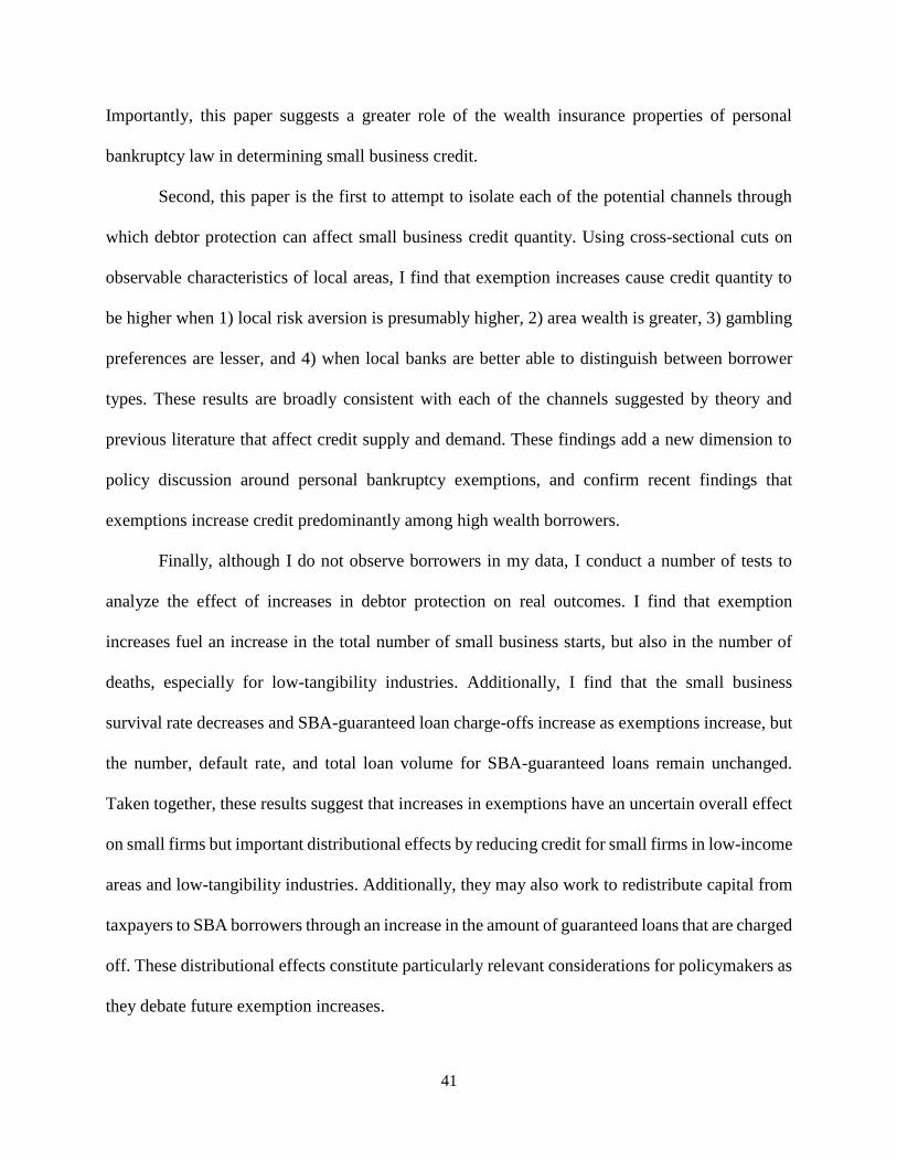
41

Importantly, this paper suggests a greater role of the wealth insurance properties of personal

bankruptcy law in determining small business credit.

Second, this paper is the first to attempt to isolate each of the potential channels through

which debtor protection can affect small business credit quantity. Using cross-sectional cuts on

observable characteristics of local areas, I find that exemption increases cause credit quantity to

be higher when 1) local risk aversion is presumably higher, 2) area wealth is greater, 3) gambling

preferences are lesser, and 4) when local banks are better able to distinguish between borrower

types. These results are broadly consistent with each of the channels suggested by theory and

previous literature that affect credit supply and demand. These findings add a new dimension to

policy discussion around personal bankruptcy exemptions, and confirm recent findings that

exemptions increase credit predominantly among high wealth borrowers.

Finally, although I do not observe borrowers in my data, I conduct a number of tests to

analyze the effect of increases in debtor protection on real outcomes. I find that exemption

increases fuel an increase in the total number of small business starts, but also in the number of

deaths, especially for low-tangibility industries. Additionally, I find that the small business

survival rate decreases and SBA-guaranteed loan charge-offs increase as exemptions increase, but

the number, default rate, and total loan volume for SBA-guaranteed loans remain unchanged.

Taken together, these results suggest that increases in exemptions have an uncertain overall effect

on small firms but important distributional effects by reducing credit for small firms in low-income

areas and low-tangibility industries. Additionally, they may also work to redistribute capital from

taxpayers to SBA borrowers through an increase in the amount of guaranteed loans that are charged

off. These distributional effects constitute particularly relevant considerations for policymakers as

they debate future exemption increases.

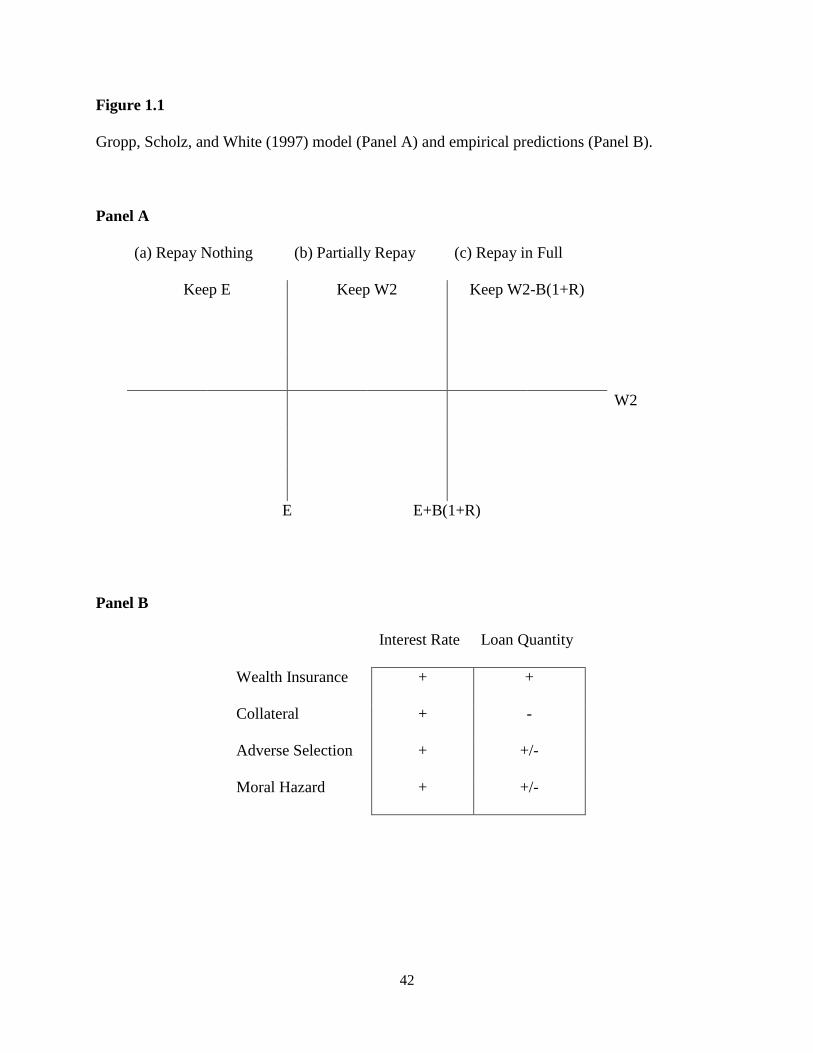
42

Figure 1.1

Gropp, Scholz, and White (1997) model (Panel A) and empirical predictions (Panel B).

Panel A

(a) Repay Nothing (b) Partially Repay (c) Repay in Full

Keep E Keep W2 Keep W2-B(1+R)

W2

E E+B(1+R)

Panel B

Interest Rate Loan Quantity

Wealth Insurance + +

Collateral + -

Adverse Selection + +/-

Moral Hazard + +/-

43

Figure 1.2

Heat map of exemption levels as of 2004.

(300000,550000](100000,300000](70000,100000]

(55000,70000](40000,55000](25000,40000](10000,25000][0,10000]

2004

Homestead Exemption Levels- US States

44

Figure 1.3

Industry breakdown based on tangibility (Net PPE/Total Assets) of COMPUSTAT firms 1999-

2004.

High-Tangibility

44-45 Retail Trade

11 Agriculture, Forestry, Fishing and Hunting

71 Arts, Entertainment, and Recreation

48-49 Transportation and Warehousing

72 Accommodation and Food Services

22 Utilities

21 Agriculture, Forestry, Fishing and Hunting

Low-Tangibility

52 Finance and Insurance

54 Professional, Scientific, and Technical Services

99 Other

42 Wholesale Trade

56 Administrative and Support

51 Information

61 Educational Services

45

Figure 1.4

Graph of dynamic effect of exemption changes on small business loan volume. Points on the

graph represent the coefficients on a dummy variable representing a change in the homestead

exemption from a regression of log small business loan volume at the state level. The dummy

variable is moved forward and backward from the actual change date at time 0 to capture

dynamic effects. All control variables, including state and year fixed effects are included in each

regression.

.02

.03

.04

.05

.06

.07

Eff

ect

on

Ln(S

B L

oa

n V

olu

me

)

-2 -1 0 1 2Years until/since Change

Graph of Dynamic Effects: Loan Volume

46

Table 1.1

Table 1.1 reports the dollar amounts for the homestead exemptions at the beginning and end of

the sample period. States with exemption levels below the Federal exemption and allowing

debtors to choose between Federal and State exemptions are assigned the Federal exemption

level for all empirical tests

Homestead Exemption Level

State 1999 2004

Alabama 10,000 10,000

Alaska 63,000 64,800

Arizona 100,000 150,000

Arkansas Unlimited Unlimited

California 75,000 75,000

Colorado 60,000 90,000

Connecticut 150,000 150,000

Delaware 0 0

Florida Unlimited Unlimited

Georgia 10,000 20,000

Hawaii 32,300 36,900

Idaho 100,000 100,000

Illinois 15,000 15,000

Indiana 15,000 15,000

Iowa Unlimited Unlimited

Kansas Unlimited Unlimited

Kentucky 10,000 10,000

Louisiana 15,000 25,000

Maine 25,000 70,000

Maryland 0 0

Massachusetts 100,000 300,000

Michigan 32,300 36,900

Minnesota 200,000 200,000

Mississippi 150,000 150,000

Missouri 8,000 15,000

Montana 120,000 200,000

Nebraska 25,000 25,000

Nevada 125,000 200,000

New Hampshire 60,000 200,000

New Jersey 32,300 36,900

New Mexico 60,000 60,000

New York 20,000 20,000

North Carolina 20,000 20,000

47

North Dakota 160,000 160,000

Ohio 10,000 10,000

Oklahoma Unlimited Unlimited

Oregon 33,000 33,000

Pennsylvania 32,300 36,900

Rhode Island 100,000 200,000

South Carolina 10,000 10,000

South Dakota Unlimited Unlimited

Tennessee 7,500 7,500

Texas Unlimited Unlimited

Utah 40,000 40,000

Vermont 150,000 150,000

Virginia 11,000 11,000

Washington 80,000 80,000

West Virginia 30,000 50,000

Wisconsin 40,000 40,000

Wyoming 20,000 20,000

Federal 32,300 40,400

48

Table 1.2

Table 1.2 reports the distribution of exemption changes across years (Panel A) and grouped by

magnitude of change (Panel B). If states increase exemptions more than once, they can be

included in the table multiple times.

Panel A

Year Increases

1999 4

2000 3

2001 8

2002 3

2003 4

2004 6

Panel B

<$10,000

$10,000<,

<$50,000 > $50,000

AK CO AZ

HI GA MA

MI LA MT

MO ME NV

NJ WV NH

PA RI

49

Table 1.3

Table 1.3 reports summary statistics for the primary variables used in the empirical tests

separated by tract, county, and state.

Variable Obs 25% Median 75% Mean Std.Dev. Min Max

Tract Variables

Ln(Total Loans) 359008 3.56 4.22 4.82 4.15 1.00 0 9.01

Ln(Large Loans) 359008 0 1.10 1.61 1.02 0.91 0 5.81

Ln(Med Loans) 359008 0 1.10 1.79 1.14 0.91 0 6.29

Ln(Small Loans) 359008 3.50 4.16 4.75 4.07 0.99 0 9.00

Ln(Total Amount) 392932 10.72 12.40 13.55 12.04 2.06 0.69 16.00

HHI 264984 0.02 0.05 0.09 0.08 0.12 0 1.00

Deposit Share (Small Banks) 264975 0.08 0.16 0.37 0.29 0.27 0 1.00

Ln(Local Lenders) 264984 3.74 5.01 5.98 4.75 1.51 0.69 7.71

County Variables

Unemp. Rate 43868 3.90 5.10 6.70 5.59 2.53 0.70 35.60

Median Income (2009 dollars) 40793 25,591 31,158 38,443 33,056 10,620 0 115,328

Population 43916 11,036 24,820 62,799 90,888 294,048 55 9,793,263

Religiosity 43914 0.47 0.62 0.77 0.63 0.21 0.02 1.86

Catholic/Protestant 41774 0.56 1.47 4.02 4.69 17.30 0 763.40

Median House Value 43940 57900 75900 96900 84623 47731 0 1000000

Median Age 43911 35.20 37.40 39.70 37.33 4.06 0 58.60

State Variables

Ln(HPI) 300 5.33 5.49 5.66 5.51 0.26 4.95 6.48

Ln(1+Homestead) 300 9.90 10.82 11.92 10.50 2.44 0 12.61

Exemption Changes 24 2550 15000 50000 32800 45647.47 900 200000

50

Table 1.4

Table 1.4 reports the results of a regression of the log total small business loans (column 1) and

log total amount of small business loans (column 2) to a Census tract on the exemption level.

Total small business loans include C&I loans or loans secured by nonfarm or non-real estate

collateral, lines of credit, and business credit card account under $1 million. Ln(1+Homestead) is

the log of the homestead exemption. Year and tract fixed effects included. Standard errors are

clustered at the state level.

(1) (2)

VARIABLES Ln(Total Loans) Ln(Total Amount)

Ln(1+Homestead) 0.05* 0.09***

(1.925) (3.182)

Constant 3.01*** 6.02***

(11.452) (19.044)

Observations 365,797 365,797

R-squared 0.593 0.150

Number of tracts 73,719 73,719

Year Yes Yes

Tract Yes Yes

Robust t-statistics in parentheses

*** p<0.01, ** p<0.05, * p<0.1

51

Table 1.5

Table 1.5 reports the results of a regression of the log total small business loans (column 1) and

log total amount of small business loans (column 2) to a Census tract on the exemption level.

Total loans and loan amount are defined as in Table 1.4. Ln(1+Homestead) is the log of the

homestead exemption. Unemployment, population, and median income are defined at the county

level, HPI is the state house price index. Year and tract fixed effects included. Standard errors

are clustered at the state level.

(1) (2)

VARIABLES Ln(Total Loans) Ln(Total Amount)

Ln(1+Homestead) 0.04* 0.09***

(1.827) (2.899)

Ln(Median Income) 0.92*** 0.41

(5.474) (1.320)

Unemp. Rate 0.01 -0.02***

(1.531) (-2.758)

House Price Growth 0.11 0.16

(0.464) (0.466)

Ln(Population) 0.20 0.20

(1.665) (1.318)

Constant -9.10*** -0.69

(-4.287) (-0.178)

Observations 344,988 344,988

R-squared 0.612 0.156

Number of tracts 72,082 72,082

Year Yes Yes

Tract Yes Yes

Robust t-statistics in parentheses

*** p<0.01, ** p<0.05, * p<0.1

52

Table 1.6

Table 1.6 reports the results of a regression of the log total small business loans (column 1) and

log total amount of small business loans (column 2) to a Census tract on the exemption level.

Total loans and loan amount are defined as in Table 1.4. Ln(1+Homestead) is the log of the

homestead exemption. Unemployment, population, and median income are defined at the county

level, HPI is the state house price index. County-pair-year and tract fixed effects included.

Standard errors are clustered at the state level

(1) (2)

VARIABLES Ln(Total Loans) Ln(Total Amount)

Ln(1+Homestead) 0.07*** 0.07**

(3.022) (2.459)

Ln(Median Income) 0.51** 0.71**

(2.202) (2.076)

Ln(Population) 0.27 0.15

(1.549) (0.483)

Unemp. Rate 0.93** 0.79

(2.496) (1.649)

House Price Growth -5.51* -2.73

(-1.750) (-0.540)

Constant

92,578 92,578

0.728 0.239

Observations 14,550 14,550

R-squared Yes Yes

Number of tracts Yes Yes

County-pair-year 0.07*** 0.07**

Tract (3.022) (2.459)

Robust t-statistics in parentheses

*** p<0.01, ** p<0.05, * p<0.1

53

Table 1.7

Table 1.7 reports the state-level regression of total number (column 1) small business loans and

total volume (column 2) by commercial banks. Small business loans and all control variables are

defined as in Table 1.4, only measured at the state-level. State and year fixed effects are

included, standard errors clustered by state.

(1) (2)

VARIABLES Ln(Total Loans) Ln(Total Amount)

Ln(1+Homestead) 0.07** 0.11***

(2.156) (3.199)

Population 0.13** 0.10*

(2.094) (1.788)

House Price Growth 0.14 0.19

(0.634) (0.982)

Unemp. Rate 0.00 -0.02

(0.016) (-1.554)

Ln(Median Income) 0.33 0.22

(1.252) (0.790)

Constant 3.80 9.15***

(1.159) (2.788)

Observations 278 278

R-squared 0.956 0.915

Number of States 48 48

Year Yes Yes

State Yes Yes

Robust t-statistics in parentheses

*** p<0.01, ** p<0.05, * p<0.1

54

Table 1.8

Table 1.8 reports the results of a regression of the small business loans to a Census tract on the

exemption level based on subsamples of high and low quartile county religiosity. Religiosity is

the number of adherents to any religion in a county in 2000 scaled by county population, taken

from the ARDA. High religiosity corresponds to high risk aversion. Total loans and loan amount

are defined as in Table 1.4. Ln(1+Homestead) is the log of the homestead exemption.

Unemployment, population, and median income are defined at the county level, HPI is the state

house price index. County-pair-year and state fixed effects included. Standard errors are

clustered at the state level. Religiosity/Risk Aversion

High Low Difference High Low Difference

Ln(Total Loans) Ln(Total Amount)

VARIABLES (1) (2) (3) (4) (5) (6)

Ln(1+Homestead) 0.24** -0.22** 0.46*** 0.30** -0.28** 0.58***

(2.579) (-2.179) (3.35) (2.707) (-2.551) (3.72)

Ln(Median Income) 1.47*** 2.30*** 1.64*** 3.00***

(8.095) (7.620) (6.528) (6.196)

Ln(Population) 0.29** 0.15 0.55*** 0.31**

(2.368) (1.672) (3.221) (2.502)

Unemp. Rate -0.11*** -0.05* -0.15*** -0.12***

(-2.796) (-1.951) (-2.786) (-2.954)

House Price Growth 1.26 -3.05** 1.07 -3.24*

(0.678) (-2.608) (0.302) (-1.938)

Constant -17.72*** -19.32*** -19.87*** -24.55***

(-8.840) (-5.271) (-6.838) (-4.190)

Observations 31,573 12,103 31,573 12,103

R-squared 0.267 0.420 0.202 0.304

County-pair-year Yes Yes Yes Yes

State Yes Yes Yes Yes

Robust t-statistics in parentheses

*** p<0.01, ** p<0.05, * p<0.1

55

Table 1.9 Table 1.9 reports the results of a regression of the small business loans to a Census tract on the

exemption level based on subsamples of high and low quartile county Catholic to Protestant

ratio. The Catholic to Protestant ratio is the number of adherents to Roman Catholicism in a

county in 2000 scaled by the number of adherents to mainline Protestant denominations, taken

from the ARDA. A high Catholic to Protestant ratio corresponds to high preference for

gambling. Total loans and loan amount are defined as in Table 1.4. Ln(1+Homestead) is the log

of the homestead exemption. Unemployment, population, and median income are defined at the

county level, HPI is the state house price index. County-pair-year and state fixed effects

included. Standard errors are clustered at the state level. Gambling Preferences

High Low Difference High Low Difference

Ln(Total Loans) Ln(Total Amount)

VARIABLES (1) (2) (3) (4) (5) (6)

Ln(1+Homestead) -0.00 0.28*** 0.28*** -0.03** 0.27*** 0.30***

(-0.254) (7.929) (7.929) (-2.066) (3.865) (4.20)

Ln(Median Income) 1.10*** 1.31*** 1.30*** 1.59***

(4.529) (8.679) (3.875) (11.193)

Ln(Population) 0.14*** 0.37*** 0.28*** 0.59***

(5.073) (6.837) (6.381) (14.143)

Unemp. Rate -0.04*** -0.03 -0.06** 0.01

(-2.744) (-0.742) (-2.383) (0.291)

House Price Growth -0.30 3.12 -2.02** 2.87

(-0.477) (1.395) (-2.368) (0.855)

Constant -8.83*** -18.65*** -8.31** -21.68***

(-3.649) (-7.011) (-2.288) (-8.066)

Observations 18,447 18,981 18,447 18,981

R-squared 0.420 0.258 0.412 0.151

County-pair-year Yes Yes Yes Yes

State Yes Yes Yes Yes

Robust t-statistics in parentheses

*** p<0.01, ** p<0.05, * p<0.1

56

Table 1.10

Table 1.10 reports the results of a regression of the log number (Columns 1 and 2) and log

amount (Columns 4 and 5) of small business loans to a Census tract on the exemption level

based on subsamples of high and low quartile county median house value (Panel A) and home

price minus the homestead level (Panel B). Median house value is taken from the 2000 Census.

Ln(1+Homestead) is the log of the homestead exemption. Unemployment, population, and

median income are defined at the county level, HPI is the state house price index. County-pair-

year and state fixed effects included. Standard errors are clustered at the state level.

Panel A Housing Prices/Collateral

High Low Difference High Low Difference

Ln(Total Loans) Ln(Total Amount)

VARIABLES (1) (2) (3) (4) (5) (6)

Ln(1+Homestead) 0.18*** 0.01 0.19*** 0.08** -0.01 0.09**

(10.087) (0.861) (8.924) (2.462) (-0.378) (2.14*)

Ln(Population) -0.59*** 0.19*** 0.09 0.32***

(-6.447) (5.920) (0.222) (7.201)

Ln(Median Income) 0.48*** 1.07*** 1.12*** 1.73***

(11.211) (4.598) (5.914) (4.406)

House Price Growth 2.02** 0.31 -0.23 0.25

(2.559) (0.858) (-0.127) (0.327)

Unemp. Rate -0.04** -0.01 -0.03 -0.05***

(-2.323) (-1.069) (-1.227) (-3.723)

Observations 20,053 23,075 20,430 23,446

R-squared 0.275 0.338 0.161 0.308

County-pair-year Yes Yes Yes Yes

Year Yes Yes Yes Yes

Robust t-statistics in parentheses

*** p<0.01, ** p<0.05, * p<0.1

Panel B Home Equity/Collateral

High Low Difference High Low Difference

Ln(Total Loans) Ln(Total Amount)

VARIABLES (1) (2) (3) (4) (5) (6)

Ln(1+Homestead) 1.43*** -0.32 1.75*** 2.13*** -0.30 2.43***

(2.952) (-1.402) (3.267) (2.728) (-1.340) (2.99)

Ln(Population) 0.71*** 0.20*** 1.09*** 0.33***

(6.382) (3.923) (6.448) (3.623)

Ln(Median Income) 1.24*** -0.09 1.31*** -0.04

(8.639) (-0.170) (6.277) (-0.036)

House Price Growth -2.77 0.31 -7.07 2.40

(-0.544) (0.132) (-0.822) (0.746)

Unemp. Rate -0.15*** -0.14*** -0.21*** -0.23***

(-3.951) (-6.196) (-3.657) (-6.626)

Constant -32.05*** 7.96 -41.12*** 9.52

57

(-7.134) (1.434) (-6.116) (0.926)

Observations 21,890 14,120 21,890 14,120

R-squared 0.281 0.420 0.176 0.385

County-pair-year Yes Yes Yes Yes

Year Yes Yes Yes Yes

Robust t-statistics in parentheses

*** p<0.01, ** p<0.05, * p<0.1

58

Table 1.11

Table 1.11 reports the results of a regression of the log C&I loans to a Census tract on the

exemption level and including an interaction between the exemption level and the number of

local lenders (column 1), and the exemption level and HHI and the percentage of bank branches

owned by large banks (column 2). Total loans, large loans, medium loans, and small loans are

defined as in Table 1.4. Ln(1+Homestead) is the log of the homestead exemption.

Unemployment, population, and median income are defined at the county level, HPI is the state

house price index. HHI, Small Mkt. Share, and Ln(Local Lenders) are defined within the 30 mile

radius circle surrounding the tract centroid County-pair-year and tract fixed effects included.

Standard errors are clustered at the state level.

(1) (2) (3) (4)

VARIABLES Ln(Total Loans) Ln(Total Amount) Ln(Total Loans) Ln(Total Amount)

Ln(1+Homestead) -0.05 -0.16*** -0.03 -0.15

(-1.050) (-2.777) (-0.354) (-1.347)

Ln(1+Homestead) * Ln(Local

Lenders) 0.03** 0.04*** 0.05* 0.08***

(2.267) (3.572) (1.906) (2.775)

Ln(1+Homestead) * % Lg. Bank -0.22* -0.29*

(-1.711) (-1.684)

Ln(1+Homestead) * HHI 0.01 0.08

(0.085) (0.385)

Ln(Median Income) 1.55*** 1.80*** 1.55*** 1.80***

(9.016) (7.441) (9.205) (7.569)

Ln(Population) 0.07*** 0.15*** 0.07** 0.14***

(2.881) (4.590) (2.657) (4.223)

Unemp. Rate -0.06*** -0.09*** -0.06*** -0.09***

(-3.204) (-3.260) (-3.268) (-3.313)

House Price Growth 1.45 1.97 1.41 1.90

(1.261) (1.176) (1.246) (1.153)

HHI -0.39 -0.55 -0.56 -1.44

(-1.293) (-1.417) (-0.300) (-0.618)

Small Bank Mkt. Share 0.42 0.34 0.41 0.32

(0.530) (0.373) (0.520) (0.358)

% Large Bank Offices 0.64 0.78 3.08 3.87

(0.665) (0.682) (1.383) (1.397)

Ln(Local Lenders) -0.22* -0.34** -0.49* -0.72**

(-1.709) (-2.214) (-1.729) (-2.350)

Constant -13.15*** -12.56*** -13.32*** -12.54***

(-6.679) (-4.522) (-6.492) (-4.311)

Observations 56,023 56,023 56,023 56,023

R-squared 0.256 0.213 0.256 0.213

County-pair-year Yes Yes Yes Yes

State Yes Yes Yes Yes

Robust t-statistics in parentheses

*** p<0.01, ** p<0.05, * p<0.1

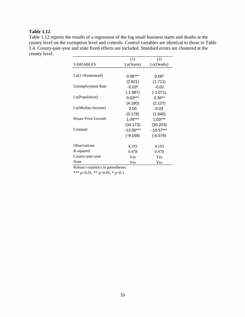
59

Table 1.12

Table 1.12 reports the results of a regression of the log small business starts and deaths at the

county level on the exemption level and controls. Control variables are identical to those in Table

1.4. County-pair-year and state fixed effects are included. Standard errors are clustered at the

county level. (1) (2)

VARIABLES Ln(Starts) Ln(Deaths)

Ln(1+Homestead) 0.08*** 0.06* (2.821) (1.711) Unemployment Rate -0.03* -0.02 (-1.987) (-1.071) Ln(Population) 0.63*** 0.36** (4.180) (2.127) Ln(Median Income) 0.00 0.03 (0.178) (1.640) House Price Growth 1.04*** 1.03*** (34.173) (30.203) Constant -13.56*** -10.57*** (-9.168) (-6.576)

Observations 4,193 4,193

R-squared 0.978 0.978

County-pair-year Yes Yes

State Yes Yes

Robust t-statistics in parentheses

*** p<0.01, ** p<0.05, * p<0.1

60

Table 1.13

Table 1.13 reports the results of a regression of the ratio of small business starts to deaths at the

county level on the exemption level and controls, based on industry tangibility. Control variables

are identical to those in Table 1.4. County-pair-year and state fixed effects are included. Standard

errors are clustered at the county level.

Tangibility

High Low

(1) (2)

VARIABLES Starts/Deaths Starts/Deaths

Ln(1+Homestead) 0.08 -0.17**

(1.353) (-2.311)

Ln(Median Income) 0.17 0.06

(1.507) (0.306)

Unemp. Rate -0.01 -0.03

(-1.325) (-1.138)

House Price Growth 0.68 -0.19

(0.982) (-0.161)

Ln(Population) -0.06*** 0.03

(-4.040) (1.019)

Constant -0.65 1.92

(-0.511) (0.783)

Observations 4,020 3,888

R-squared 0.549 0.567

County-pair-year Yes Yes

State Yes Yes

Robust t-statistics in parentheses

*** p<0.01, ** p<0.05, * p<0.1

61

Table 1.14

Table 1.14 reports the results of a regression of the survival rates of small firms in started in year

t at the state level on the exemption level and controls. Control variables are identical to those in

Table 1.4, only measured at the state level. Year and state fixed effects are included. Standard

errors are clustered at the state level.

(1) (2) (3)

VARIABLES 1 yr. survival rate 2 yr. survival rate 3 yr. survival rate

Ln(1+Homestead) -1.46*** -1.45*** -1.44*

(-2.778) (-2.701) (-1.862)

Ln(Population) 1.88 1.62 1.78

(1.162) (0.761) (0.772)

House Price Growth -0.98 -2.85 -0.25

(-0.218) (-0.532) (-0.051)

Unemployment Rate -0.95*** -0.91*** -0.74**

(-3.221) (-2.774) (-2.141)

Ln(Median Income) 2.94 -4.67 -3.51

(0.380) (-0.606) (-0.413)

Constant 32.85 106.43 81.71

(0.349) (1.095) (0.759)

-1.46*** -1.45*** -1.44*

Observations (-2.778) (-2.701) (-1.862)

R-squared 1.88 1.62 1.78

Number of States (1.162) (0.761) (0.772)

Year -0.98 -2.85 -0.25

State (-0.218) (-0.532) (-0.051)

Robust t-statistics in parentheses

*** p<0.01, ** p<0.05, * p<0.1

62

Table 1.15

Table 1.15 reports the results of a regression of the log of SBA loan defaults (column 1), the log

of the number of SBA loans (column 2), the log of the total amount of SBA loans (column 3),

and the log of total charged off amount (column 4) at the state level on the exemption level and

controls. Control variables are identical to those in Table 1.4, only measured at the state level.

Year and state fixed effects are included. Standard errors are clustered at the state level.

(1) (2) (3) (4)

VARIABLES Ln(SBA Defaults) Ln(SBA Loans) Ln(SBA Amount) Ln(SBA Amount Chg. Off)

Ln(1+Homestead) 0.21 0.06 0.04 0.24*

(1.408) (0.729) (0.846) (1.873)

Population 0.36 0.38** 0.20* 0.15

(1.299) (2.029) (1.875) (0.616)

House Price Growth 1.76* 0.38 -0.14 2.56***

(1.747) (0.588) (-0.272) (3.005)

Unemp. Rate 0.14** 0.09** 0.03 0.14***

(2.664) (2.518) (1.097) (3.067)

Ln(Median Income) -0.48 -0.55 -0.42 -0.96

(-0.410) (-0.871) (-0.976) (-0.743)

Constant -0.49 3.91 18.73*** 19.81

(-0.036) (0.491) (3.520) (1.353)

Observations 276 276 276 276

R-squared 0.612 0.717 0.533 0.240

Number of States 48 48 48 48

Year Yes Yes Yes Yes

State Yes Yes Yes Yes

Robust t-statistics in parentheses

*** p<0.01, ** p<0.05, * p<0.1

63

Table 1.16

Table 1.16 reports the results of a regression of the log total small business loans (column 1) and

log total amount of small business loans (column 2) to a Census tract on the exemption level.

Total loans and loan amount are defined as in Table 1.4. Ln(1+Homestead) is the log of the

homestead exemption. Unemployment, population, and median income are defined at the county

level, HPI is the state house price index. HHI, Small Bank Deposit Share, and Ln(Local Lenders)

are defined using Summary of Deposits data, and calculated within the 30 mile radius circle

surrounding tract centroids. Year and tract fixed effects included. Standard errors are clustered at

the state level.

(1) (2)

VARIABLES Ln(Total Loans) Ln(Total Volume)

Ln(1+Homestead) 0.03 0.07***

(1.529) (3.049)

Ln(Median Income) 0.94*** 0.60***

(3.997) (2.754)

Ln(Population) 0.07 0.12

(0.587) (0.890)

Unemp. Rate -0.01* -0.03**

(-1.768) (-2.315)

House price growth -0.08 0.49

(-0.398) (1.351)

HHI -0.20*** -0.11

(-3.007) (-0.991)

Small Bank Mkt. Share 0.02 0.12

(0.382) (1.432)

% Large Bank Offices 0.15** 0.26**

(2.141) (2.272)

Ln(Local Lenders) -0.00 0.08

(-0.152) (1.344)

Constant -7.29*** -2.07

(-2.920) (-0.764)

Observations 252,570 252,570

R-squared 0.376 0.141

Number of tracts 60,390 60,390

Tract Yes Yes

Year Yes Yes

Robust t-statistics in parentheses

*** p<0.01, ** p<0.05, * p<0.1

64

Table 1.17

Table 1.17 reports the results of a regression of the log total number and total amount of small

business loans on an exemption change dummy, as well as placebo dummies coinciding with the

year prior and year following the change. Year and tract fixed effects are included. Standard

errors are clustered at the state level.

(1) (2)

VARIABLES Ln(Total Loans) Ln(Total Amount)

Placebo t-1 0.00 -0.00

(0.065) (-0.080)

Exempt. Change 0.01 0.08**

(0.752) (2.049)

Placebo t+1 -0.00 0.02

(-0.121) (0.293)

Ln(Median Income) 0.93*** 0.43

(4.930) (1.232)

Unemp. Rate 0.01 -0.02**

(1.136) (-2.471)

House Price Growth 0.12 0.10

(0.414) (0.224)

Ln(Population) 0.23* 0.23

(1.729) (1.200)

Constant -9.16*** -0.31

(-3.976) (-0.069)

Observations 280,893 280,893

R-squared 0.604 0.153

Number of tracts 59,250 59,250

Tract Yes Yes

Year Yes Yes

Robust t-statistics in parentheses

*** p<0.01, ** p<0.05, * p<0.1

65

Table 1.18

Table 1.18 reports the results of a regression of the average SBA initial interest rate (column 1)

and the SBA average maturity (column 2) on the exemption level. Control variables are identical

to those in Table 1.4, and also include the average amount guaranteed by the SBA. Year and tract

fixed effects are included. Standard errors are clustered at the county level.

(1) (2)

VARIABLES Avg. Int. Rate Avg. Maturity

Ln(1+Homestead) 0.25** -3.18*

(2.354) (-1.691)

Avg. SBA Guar. 0.92*** -67.56***

(6.076) (-16.721)

Unemp. Rate -0.85 -14.58

(-1.649) (-1.094)

Ln(Population) -3.42** -4.38

(-2.576) (-0.269)

Ln(Median Income) -0.01 1.00*

(-0.184) (1.681)

House Price Growth -0.03 23.94*

(-0.037) (2.000)

Constant 52.60*** 436.75**

(3.198) (2.291)

Observations 9,632 12,192

R-squared 0.817 0.168

Number of tracts 2,783 2,979

Year Yes Yes

County Yes Yes

Robust t-statistics in parentheses

*** p<0.01, ** p<0.05, * p<0.1

66

Table 1.19

Table 1.19 reports the results of a regression of loans to small businesses with annual revenue <

$1 million in a Census tract on the exemption level. Ln(1+Homestead) is the log of the

homestead exemption. Unemployment, population, and median income are defined at the county

level, HPI is the state house price index. Tract and year fixed effects included. Standard errors

are clustered at the state level.

(1) (2)

VARIABLES Ln(Total Loans) Ln(Total Amount)

Ln(1+Homestead) 0.04* 0.08***

(1.849) (2.988)

Ln(Median Income) 0.66*** 0.35

(4.346) (1.252)

Ln(Population) -0.01 -0.02**

(-0.981) (-2.126)

Unemp. Rate 0.35 0.50

(1.250) (1.167)

House Price Growth 0.39*** 0.41*

(2.791) (1.920)

Constant -9.22*** -3.37

(-4.387) (-0.752)

Observations 344,988 344,988

R-squared 0.8807 0.754

Tract 72,082 72,082

Year Yes Yes

Robust t-statistics in parentheses

*** p<0.01, ** p<0.05, * p<0.1

67

Chapter 2

INFORMATION ASYMMETRY AND ORGANIZATIONAL STRUCTURE: EVIDENCE

FROM SMALL BUSINESS LENDING

2.1 Introduction

How do the characteristics of the project, such as the importance of soft information, determine

the optimal organization of the firm? This is the central question of Stein (2002), who contrasts

two types of organizations: “decentralized” and “hierarchy”. He notes the comparative advantage

of flatter organizational forms over their hierarchical peers others in processing soft information,

and therefore in certain production technologies. In this paper I empirically examine this question

in a unique setting where the soft information about the borrower is particularly important.

Specifically, I use staggered increases in the amount of assets that borrowers can shield from

unsecured creditors in bankruptcy as an exogenous shock to the screening incentives of lenders to

small businesses.

Little empirical work can currently attribute a causal effect of information frictions on the

organizational characteristics of market participants. This is likely due to several factors. First,

exogenous shocks to information are difficult to find and quantify. Second, proxies for information

are likely affected by unobservable economic forces that jointly determine organizational

structure. This paper utilizes staggered increases in state-level personal bankruptcy exemptions

which exacerbate the adverse selection and moral hazard problems facing small business lenders,

and increase the importance of soft information in the decision to provide credit. Combined with

comprehensive data on small business credit provision by commercial banks, I can examine the

effect of an increased importance of soft information on the organizational structure of essentially

all participants in this large market. Such analysis can inform policy, both in terms of relevant

markets for antitrust regulation, and in terms of adverse effects of debtor protection.

68

Small business lending presents an ideal setting for examining the effect of information

frictions on organizational structure. Unlike their larger, public counterparts, small businesses

generally lack audited financial statements and well-defined financial histories that mitigate the

information asymmetry with the capital markets. In addition, the ease by which the entrepreneur

can shuttle funds between business and personal accounts often blurs the distinction between the

business and the individual, increasing the scope for moral hazard and the cost of adverse selection.

In this setting, information regarding the entrepreneur’s personal character and the local economic

environment in which she operates, what Stein (2002) calls ‘soft information’, become particularly

important.

To examine the effect of soft information on the organizational structure of lending banks I

use state-level changes in personal bankruptcy exemptions, which determine the amount of assets

that individual debtors can shield from unsecured creditors during bankruptcy. Personal

bankruptcy law also represents the relevant bankruptcy system for small businesses since, for non-

corporate businesses, business debt remains a personal liability of the owner. In addition, owner

personal finances are generally indistinguishable from business accounts due to the ease of

transferring funds between sources. Importantly, though personal bankruptcy exemptions directly

affect small businesses, the reasons for their increase are largely exogenous to the structure of local

financial markets.

Since bankruptcy exemptions shield assets from creditors in the event of bankruptcy, they act

as a form of partial wealth insurance for individuals. Debtors value this insurance as it lowers the

expected cost of an extreme adverse wealth shock and subsequent bankruptcy. These exemptions

therefore have immediate implications for both the supply of and demand for credit. On the

demand side, risk-averse borrowers are better off with the partial wealth insurance and demand

69

more debt, all else equal. On the supply side, lenders expect 1) the debtor to choose riskier projects

(or bankruptcy) in the face of this lower expected cost of bankruptcy and 2) worse borrowers in

general to enter the credit market.36

The two supply side effects noted above describe the frictions that characterize small business

lending markets first highlighted by Stiglitz and Weiss (1981). These frictions, moral hazard and

adverse selection, arise out of the inherent information asymmetry between lenders and borrowers

in small business lending markets and contribute to credit rationing in equilibrium.37 Personal

bankruptcy exemptions therefore heighten the information asymmetry problems in small business

lending and the screening incentive of lenders by both inducing riskier project choice (moral

hazard), and by generally reducing the expected quality (in terms of repayment propensity) of the

borrower pool (adverse selection).

Importantly, the literature on personal bankruptcy finds considerable heterogeneity in the

propensity of individuals to file for bankruptcy, holding the level of the financial benefit constant

(White 1998). This heterogeneity is broadly described as “stigma” and is usually described as a

function of social and cultural variables. Thus, even as the financial benefit of exemptions

increases, certain individuals are less likely to file for bankruptcy than others, and this propensity

relies directly on soft information about the borrower.

As my primary measure of bank organizational structure, I focus on the physical distance

between the borrower (the source of the soft information) and the lender headquarters (the

decision-making center). This measure recognizes the crucial role of the headquarters as the

36 Fan and White (2002) confirm this theory in their study of entrepreneurship. They find that self-employment is

higher in high exemption states, but can decrease if exemptions rise sufficiently high as the supply effect begins to

dominate. 37 The basic intuition of this model is, since the interest rate affects the quality of the borrower pool and borrower

risk-taking behavior, it cannot clear the market.

70

ultimate decision center of the bank, and highlights the importance of distance to headquarters as

a measure of organizational hierarchy that is specific to each borrower. My focus on borrower-

headquarter distance is driven by the recent growth in papers citing the importance of this

“functional distance” for local economic growth (Alessandrini et al (2005)), bank efficiency

(Berger and DeYoung (2001)), and local firm innovation (Alessandrini, Presbitero, and Zazzaro

(2009)). In addition, Udell (1989) notes that banks employ loan review departments to monitor the

health of their loan portfolios, and finds that these departments arose as a response to agency

problems within the bank. This indicates that bank headquarters still act as the ultimate arbiter of

branch lending decisions, even for geographically dispersed banks.

Consistent with predictions of theories of information type and organization structure, I find

that increases in the importance of soft information in a local market decrease the average distance

between borrowers and lender headquarters. Specifically, I find that the average distance between

borrowers and lender headquarters shrinks 2.8-3.7% for an average increase in exemptions, while

the proportion of lending banks with a branch within 30 miles of the Census tract does not change.

These results are consistent with the intuition that flatter organizations are better able to produce

and utilize soft information when exemptions increase.

Extrapolating from this intuition, the empirical banking literature often uses bank size as a

proxy for the ability of lenders to generate and utilize soft information about borrowers (Berger

and Udell (2002), Berger et al (2005)). Smaller banks are thought to have fewer levels of hierarchy,

and thus to give agents greater autonomy in allocating credit. To the extent that this assumption is

correct, increases in the importance of soft information should also reduce the average size of

lenders catering to a market, all else equal. I find no evidence of a shift to smaller banks after

exemptions increase. However, I find that the decrease in average lending distance within a local

71

market is concentrated among large banks, indicating that bank size may imperfectly substitute for

geographic dispersion in mitigating information frictions. These results may help to explain

conflicting results in the empirical banking literature (see e.g. Berger et al. (2014)) inasmuch as

bank size is a noisy proxy for organizational structure.38 These results also suggest that the

borrower-centric measure of distance to headquarters more accurately captures the degree of

information asymmetry.

Borrowing from the literature on the determinants of filing for bankruptcy (see e.g. Sullivan,

Warren, and Westbrook (1987), Brinig and Buckley (1996), White (1998), Fan and White (2002)),

I find that social and cultural factors generally described as ‘stigma’ found to be important

determinants of the decision to file for bankruptcy (namely, whether the tract is rural or urban and

the proportion of religious organizations) significantly alter the effect of increases in exemptions

on the average lending distance of banks to local small businesses. More specifically, social and

cultural variables that mitigate moral hazard problems for lenders reduce the number of strategic

filers that enter the market when exemptions increase. As a result, an increase in exemptions

entices fewer low type borrowers to the market, and the relative information costs for distant

lenders vs. local lenders remain relatively unchanged. Consistent with this intuition, I find that the

magnitude of the decrease in average distance between borrowers and lenders is much smaller in

rural markets or in markets with a high proportion of religious organizations.

This paper builds on the literature begun in large part by Berger and Udell (2002) and Stein

(2002). Stein (2002) shows that certain organizational forms have a comparative advantage in

industries where information asymmetry is severe and soft information dominates. In these

38 I also test the effect of personal bankruptcy exemptions on other traditional measures of organizational structure

used in the banking literature such as the percent of unit banks, multi-bank holding companies, and multi-market

banks. I find no evidence of a shift utilizing these other measures.

72

markets, flatter organizations, where the decision-making power is located closer to the

information production, maintain a comparative advantage over their hierarchical competitors.

Hauswald and Marquez (2006) develop a model with similar intuition in which the quality of a

bank’s information generation process decreases with distance, and local banks therefore maintain

an information advantage over their distant peers. Furthermore, this comparative advantage is

increasing in the proportion of ‘low’ type borrowers. These models show that the degree of

information asymmetry plays a critical role in determining the dominant organization form,

whether described by ‘organizational distance’ or geographic dispersion, and therefore must also

play a critical role in the determination of industry structure.39

This paper also contributes to the literature concerning the determinants of the distance

between small borrowers and lenders and its effect on real outcomes. Petersen and Rajan (2002)

find that lending distance is increasing over time, and conclude that technology is “breaking the

tyranny of distance, at least in small business lending” (pg. 2535). In a similar vein, DeYoung,

Glennon, and Nigro (2006) find that banks’ use of credit scoring technologies increases the

distance of lending. Degryse and Ongena (2005) use data from a large Belgian bank to show that

the interest rate on loans is decreasing in the distance to the bank and increasing in the distance

between the bank and its nearest competitor. Most recently and most related to this paper, Agarwal

and Hauswald (2010) find that the inclusions of a bank’s proprietary information in a regression

of loan characteristics on distance and controls renders the coefficient on distance insignificant.

This indicates that distance is only important inasmuch as it relates to bank information. Unlike

Agarwal and Hauswald (2010), I use a comprehensive data set of credit provision to small

businesses. This allows me to examine the impact of information asymmetry on the proximity of

39 Berger and DeYoung (2001) use the term organizational distance to describe the distance between parent and

affiliate in US bank holding companies.

73

small business credit markets as a whole, and also the differential effect of information asymmetry

across bank types. In addition, I show how the general structure of local credit markets vis-à-vis

proximity of bank headquarters affects the provision of credit and small business outcomes when

information asymmetry increases.

Other papers have examined the effect of personal bankruptcy exemptions on entrepreneurship

(Fan and White (2002)), credit access (Gropp, Scholz, and White (1997)), loan terms (Berkowitz

and White (2004), Berger, Cerqueiro, and Penas (2011)), small business capital structure

(Cerqueiro and Penas (2014)), household debt (Brown, Coates, and Severino (2014)), aggregate

small business credit (Hackney (2015)), and innovation (Cerqueiro et al. (2014)). I apply the

exemptions in a novel setting where the resulting increase in the importance of soft information

for lenders presents an ideal laboratory for examining the effect of information types on

organizational structure. The staggered nature of bankruptcy laws provides multiple quasi-natural

experiments, and thus allows for robust empirical testing. I extend this literature by utilizing these

laws to address a fundamental question in economics- how do characteristics of the project, such

as the importance of soft information, determine the optimal organization of the firm?

The results suggest that particular organizational structures fare better when soft information

becomes more important. The ability to process valuable soft information about borrowers’

propensity to repay, which, at an aggregate level, is largely a function of local economic and social

characteristics, gives local lenders a comparative advantage over their distant counterparts that is

increasing in the exemption level. Local banks whose power to allocate capital resides closer to

the production of soft information can more easily mitigate information frictions brought on by

increases in exemptions, and lending becomes more local in response.

74

The rest of the paper is organized as follows. Section II describes the function of personal

bankruptcy exemptions and their political economy, Section III describes the theoretical

motivation, Section IV presents the data, empirical methodology, and results, Section V

robustness, and Section VI concludes.

2.2 Personal bankruptcy exemptions

Although the bankruptcy procedure for consumers in the US is uniform across states, states

decide the amount of assets that borrowers can shield from creditors in the event of bankruptcy.

The US personal bankruptcy system distinguishes between two primary types of bankruptcy:

Chapter 7 and Chapter 13.40 Chapter 7 allows for a complete discharge of all unsecured debts while

Chapter 13 allows only a partial discharge and requires the debtor to arrange a payment schedule

with creditors over the following 3-5 years. Under Chapter 13, creditors can also garnish future

wages, while this practice is restricted under Chapter 7. I will be focusing in this case on

exemptions that apply under Chapter 7.

State exemption statutes vary widely in their form and substance. Exemptions are divided into

two primary groups: personal property and homestead. Personal property exemptions cover

anything from wedding rings to livestock to motor vehicles, while homestead exemptions

determine the amount protected in the form of home equity. Usually, the exemption amounts are

specified in dollar amounts, but sometimes refer instead to specific items (such as a family bible

or home furnishings), or in the case of land, acreage. This is especially true of personal property

exemptions, which differ dramatically in the coverage of assets and the specificity of their value.

Personal exemptions also vary little across states and over time. Due to the difficulty of quantifying

40 See Hackney (2015) for a more complete description of chapter types.

75

the value of personal exemptions and the fact that the homestead exemption represents the bulk of

the protected value during bankruptcy and the bulk of the variation in exemption levels, I focus on

homestead exemption levels in the following tests.41

Table 2.1 shows the levels of the homestead exemption in each state as well as the federal

exemption over the period 2000-2009. As the table shows, states exhibit wide time-series and

cross-sectional variation in homestead exemption levels. Seven states do not limit the amount of

equity that the debtor can shield in home equity during bankruptcy, and four do not shield any

home equity.42 Over the nine-year time window, 24 states increased their exemption levels, with

the cumulative increases ranging from $7,200 (Alaska) to $425,000 (Nevada). The median

increase over this time window was $25,000, which is almost 40% of the median homestead

exemption. The exemption increases also appear to be fairly evenly distributed across the time

window (Table 2.2). Each year in the sample sees at least 2 exemption increases, and the maximum

number of increases in a single year is 11 in 2005. In total, states increased exemptions 55 times

from 2000 to 2009.

Lawmakers often site the increase in house prices as a motivation for increasing the homestead

exemption (Cerqueiro and Penas (2014)). Increasing housing prices are often the result of a

burgeoning local economy, and increase small business starts (Adelino, Schoar, and Severino

(2015)). This effect is driven by the increase in the collateral value of the home and is most

pronounced where this increased collateral value is sufficient to fund operations (low capital-

intensive industries). If increasing housing prices drive entrepreneurial activity and startup firms

41 This follows closely to previous literature examining the effect of personal bankruptcy exemptions (Gropp (1997),

Berger, Cerqueiro, Penas (2011)). 42 This refers to 2000 exemption levels. Delaware subsequently increased its homestead exemption from 0 to

$50,000. It should also be noted that in each of these states, the debtor can choose between state and federal

exemptions, making the federal homestead exemption level the relevant amount.

76

are more likely to borrow from local lenders, then housing prices, rather than information frictions,

may be driving both the decision to increase exemptions and the shrinking distance between

borrowers and lenders. However, two observations mitigate this concern. First, I measure lending

distance at the Census tract level, where local housing prices are unlikely to drive state policy.

Second, increased house prices are also associated with greater lending distance (DeYoung,

Glennon, and Nigro (2006)). The posting of collateral lessens the scope for moral hazard and

thereby softens information frictions, allowing lenders to lend at a greater distance. Therefore, the

overall predicted effect of increased house prices on lending distance is unclear. Nevertheless, to

control for local economic conditions, I include county median income, unemployment, and

business starts as well as the state house price growth computed from the Federal Housing Finance

Administration (FHFA) data in the main empirical tests.

From an empirical standpoint, if bankruptcy exemptions somehow correlate with, for example,

other economic conditions that affect lending distance, then I may erroneously attribute any effect

to the changing of exemptions. Importantly for my setting, therefore, two recent papers examine

the relationship between the exemption level and local macroeconomic conditions. First, Hynes,

Malani, and Posner (2004) examine the determinants of state exemption levels and find that the

exemption level in 1920 is the only robust predictor of current exemption levels, suggesting that

exemptions are exogenous to local economic conditions in the cross-section. Second, Brown,

Coates, and Severino (2014) examine the relationship between state-level variables such as house

prices, medical expenses, GDP, and filing rates, and find that changes in these variables do not

predict changes in the exemption level. Therefore, following these papers I assume that exemptions

are exogenous to local economic variables that could also be driving changes in lending behavior.

77

2.3 Theory and empirical predictions

Berger and Udell (2002) and Stein (2002) were among the first to note the importance of

organizational structure in determining the production technologies of firms. Stein (2002) presents

a model in which certain types of organizations possess a comparative advantage in generating

and utilizing ‘soft information’. According to Stein (2002), ‘soft information’ is “information that

cannot be directly verified by anyone other than the agent who produces it” (pg. 1892). As a result,

agents who produce the soft information must also have the power to allocate capital based on

their research. If this were not the case, agents would need to pass on the soft information to

decision makers, who would subsequently discount it due to its unquantifiable and unverifiable

nature. As a result, agents have no ex ante incentive to produce the soft information when they do

not also have capital allocation power. This theory then predicts that flatter organizational

structures, where the decision to allocate capital is centralized with the production of soft

information, will have a comparative advantage in markets where this information is particularly

important for the efficient allocation of capital. Similar intuition applies when looking at the

physical distance between the production of soft information and decision making power. Similar

to passing information up the levels of hierarchy, agents cannot easily pass soft information over

large physical distances. Decision makers located far from the production of soft information

cannot readily verify and therefore utilize it, giving lenders with local decision making a

comparative advantage in processing the soft information, all else equal.43

In the context of personal bankruptcy law, if increased information frictions brought on by

increases in exemptions do not affect the relative importance of soft information and thereby,

screening, then they should also have no effect on the average distance between borrowers and

43 As evidence of the local nature of small business, Petersen and Rajan (2002) note that the average (median)

distance between a small business borrower and its lender branch is 114 (9) miles over their sample period.

78

bank headquarters. Put differently, if increased exemptions increase adverse selection and moral

hazard costs equally across distant and local lenders, then we would not expect a change in the

composition of local vs. distant lenders. However, if information frictions disproportionately affect

distant lenders by increasing the value of soft information and thereby the competitive advantage

of local lenders, then we would expect a decrease in the average lending distance to a local market

(a compositional shift to local lenders).

A number of theoretical and empirical papers suggest that the relative importance of soft

information does in fact increase when exemptions increase. White (1998) presents a simple model

in which two types of borrowers face identical pre-exemption income distributions but react

differently to changes in exemptions. One group only files for bankruptcy when pre-exemption

income falls below a certain threshold defined as the “general exemption” (Type A). The other

group, the strategic filers, effectively ‘plan’ for bankruptcy and preemptively shift assets from

nonexempt to exempt categories, effectively increasing the gain from filing and filing in more

states of the world (Type B). Even though both types of borrowers have the same pre-exemption

income distribution, the probability of repayment for Type B borrowers is lower. When

exemptions increase, the expected financial benefit of bankruptcy entices a higher proportion of

Type B borrowers, exacerbating adverse selection for lenders. White (1998) provides empirical

support for this distinction between borrower types. She finds that at least 15% of US households

could financially benefit from filing for bankruptcy, but the actual filing rate is only 1% of

households. This in turn reveals that the costs of bankruptcy, both pecuniary and non-pecuniary,

play a significant role in the decision to file, and affect the magnitude of the moral hazard and

adverse selection problems facing lenders.

79

The differences between borrower types can be cast in social or cultural attitudes towards

bankruptcy. Indeed a large number of empirical papers note the importance of social and cultural

factors in predicting bankruptcy rates (see e.g. Buckley and Brinig (1998), Fay, Hurst, and White

(2001), Beck et al. (2012)). Borrowers weigh the financial benefits of bankruptcy against the costs,

which not only include financial disincentives such as increased costs of future borrowing, but also

the costs associated with stigma, all of which vary by borrower. Certainly these borrower

characteristics, along with other factors such as borrower integrity and local economic conditions,

constitute relevant information that could potentially allow lenders to distinguish between Type A

and Type B borrowers ex ante. Further, since this information is inherently soft, it represents an

opportunity for lenders with a comparative advantage in generating and processing soft

information to gain market share. Therefore, as exemptions increase and more Type B borrowers

enter the market, the relative importance of soft information increases, and so too does the

comparative advantage of local lenders.

Hauswald and Marquez (2006) solidify this notion in a model where the quality of the lender’s

signal of borrower type is decreasing in the distance to the borrower. They show that as the

proportion of ‘low’ type borrowers increases in the market (as it does with increases in personal

bankruptcy exemptions), the importance of screening increases and the adverse selection problem

worsens, especially for distant borrowers. This theory then predicts that an increase in the

information frictions facing lenders vis-à-vis exemption increases should decrease the average

distance between borrowers and lenders due to the relative increase in cost for distant lenders.

The analysis has thus far ignored the role of the price of credit and other contractual levers as

tools to clear the lending market. Certainly adjustment occurs along many margins when

exemptions increase. Lenders can increase the price of credit, increase collateral requirements,

80

shorten maturities, decrease loan amounts, or generally tighten the terms of credit to reflect the

increased risk.44,45 A crucial assumption of this analysis then is that these are not perfect substitutes

for the proximity of bank headquarters. In addition, the analysis that follows will show that these

costs do not rise proportionately for local and distant lenders. Therefore, abstracting from the

specific contractual arrangements between lenders and borrowers, increases in information

frictions should affect the types of organizations willing to serve this opaque market through their

differential impact on the cost of lending.

Prediction 1: Increases in exemptions increase the comparative information advantage of local

lenders, and decrease the distance between borrowers and lender headquarters on average.

The model of Stein (2002) shows that agents with the power to allocate capital are

incentivized to produce valuable soft information since they have the power to act on it. The flatter

organizational structures necessary to promote such capital allocation power cannot be easily

scaled up due to increasing agency costs, and therefore these flatter organizations are also

necessarily smaller. Therefore, to the extent that small banks have flatter organization structures

and therefore locate decision making power closer to soft information production (Stein (2002)),

we would also expect to see the size of the lender shrink on average when information frictions

increase.

44 In their seminal model, Stiglitz and Weiss (1981) show that, under reasonable assumptions and in the presence of

information asymmetry, the interest rate may not clear the market and thus credit rationing can occur in equilibrium.

This result persists even when collateral is introduced. 45 Berger, Cerqueiro, and Penas (2011) show that increases in personal bankruptcy exemptions result not only in

increased interest rates but also in increased collateral requirements and shorter loan maturities.

81

Prediction 2: Increases in information frictions increase the comparative advantage of small banks

with flatter organizational structures, and lending bank size becomes smaller on average.

If this prediction bears out, it lends further credence to the use of bank assets as a proxy for

the ability of banks to process soft information (see e.g., Berger and Udell (1998), Berger et al.

(2005)). If size (as a proxy for organization structure) is even an imperfect substitute for the

distance between borrowers and capital allocation decision-making power, then there may be a

differential effect of increased information frictions on the lending distance of large and small

banks. More specifically, large banks lending to a particular location should be closer following

increases in exemptions, while the lending distance of small banks should see a smaller, if any,

change.

Prediction 3: The lending distance of large banks should see a greater decrease than that of small

banks following an increase in exemptions.

If increases in exemptions cause small business credit markets to be more local, then they

may also affect outcomes for small businesses. Areas with bank headquarters located farther away

ex ante could be differentially affected by increases in exemptions. If fewer local lenders exist to

support small firms following exemption increases, then these increases may result in adverse

outcomes (in the form of fewer starts and expansions, and more contractions and deaths) for local

firms. More specifically, conditional on the distance to bank headquarters of local branches, fewer

small businesses should enter the market and fewer should expand operations when exemptions

82

increase. Further, if credit becomes more scarce when distant banks exit, small businesses may

reduce operations or exit the market entirely.

Prediction 4: Areas where branch headquarters are located farther away should see a deterioration

of small business outcomes following an increase in exemptions, all else equal.

The above discussion of various cultural attitudes towards bankruptcy also points to other

interesting cross-sectional tests. For example, if the cultural stigma towards bankruptcy in a

particular region is high, the increase in financial incentives may be insufficient to overcome the

social cost of bankruptcy.46 In this setting, an increase in exemptions would entice fewer low type

borrowers to the market, and the relative information costs for distant lenders vs. local lenders

would remain relatively unchanged.

Prediction 5: Exemptions decrease lending distance less in areas where bankruptcy carries a

greater stigma.

2.4 Data and empirical methodology

2.4.1 Data

I collect data from multiple, primarily public, sources. Data on small business loans comes

from the FFIEC by way of the Community Reinvestment Act (CRA). This act mandates the annual,

aggregate reporting of small business lending for banks over a certain size, and requires banks to

report the location of business that receives the loan. The FFIEC changed its minimum asset

46 Brinig and Buckley (1996) and Fan and White (2002) find evidence consistent with ‘stigma’ affecting the decision

to file.

83

threshold in 2005 from $250 million to $1 billion.47 This feature of the data is important since

Berger et al (2005) find that large banks tend to lend at a larger physical distance and interact with

borrowers more impersonally. In addition, Brevoort and Hannan (2004) find that the increase in

lending distance over time is driven by large banks. I examine how this particular facet of the data

affects my results in detail below using subsamples based on both time windows and bank size.

For bank balance sheet and location information, I use the FDIC Call Report and Summary of

Deposits (SOD) data, respectively. SOD data provide both the deposits and location at the

commercial bank branch-level, as well as total assets for the bank institution and location of

institution headquarters. Data on county small-business starts, unemployment, and median income

come from the BEA, state house prices from the FHFA, and county population from the Census.

I collect homestead exemption changes primarily from two sources. First, I use various editions

of How to File for Chapter 7 Bankruptcy to note yearly changes in exemption levels by state. I

then verify the timing of these changes by referencing the individual state statutes governing the

changes and the particular state legislative sessions in which they were amended. This second step

results in several changes to the values reported in the appendix of the book, but overall confirmed

the reported timing of exemption level changes.

I focus my analysis on Census tracts. Census tracts are arbitrary sub-regions of a county drawn

by the Census Bureau in order to provide a stable region for the presentation of statistical data.

These tracts vary in population from 1,200 to 8,000 residents but “ideally” contain 4,000. Due to

this fact, census tracts vary widely in geographical size depending on the density of the population.

The average land area of a Census tract in the sample is roughly 50 square miles, but the median

land area is only 2.79 square miles. This latter observation lends credence to the use of census tract

47 Greenstone, Mas and Nguyen (2014) estimate that these larger banks made up roughly 86% of small business

lending in 2007.

84

centroids as a rough proxy for borrower location and cuts down the noise from imperfectly

measuring distance between borrower and lender. Tracts remain relatively stable over the course

of time, but can change due to population shifts at a new decennial census. For this reason, I focus

on the years 2000-2009, during which tract boundaries do not change.

To obtain the average distance between borrowers and lenders I begin by compiling the

geographic centroids of Census tracts. These centroids are provided by the Census Gazeteer files,

and represent the center point of a minimum bounding rectangle. I obtain the addresses of bank

branch and institution headquarters from the FDIC Summary of Deposits data. For many of the

bank branches, the SOD data also provides latitude and longitude coordinates. For branches

missing these coordinates, I take the addresses of both bank branches and institution headquarters

and assign latitude and longitude coordinates using SAS software and Census TIGER files.

After assigning latitude and longitude coordinates to every bank branch and institution

headquarters, I calculate the distance between those banks identified by the CRA data as lending

to a particular Census tract in a given year and the tract centroid using an approach introduced by

Thaddeus Vincenty (Vincenty 1975). This method calculates the geodesic distance between two

points on the Earth’s surface assuming an ellipsoid, rather than spherical, shape. Following

Petersen and Rajan (2002), I winsorize this distance at the upper 1% to ensure comparability with

models of small business lending.48 Finally, I take the average distance between each bank

institution headquarters that lends to a particular Census tract and the tract centroid for each tract-

year. The average (median) lending distance in the sample is roughly 800 (747) miles. Summary

statistics for these variables and all controls are reported in Table 2.3.

48 Results are unchanged if I do not winsorize.

85

2.4.2 Empirical model

To test the effect of increased information frictions via increases in state personal bankruptcy

exemption levels on the distance of economic exchange I estimate the following baseline model:

𝐴𝑣𝑒𝑟𝑎𝑔𝑒 𝐿𝑒𝑛𝑑𝑖𝑛𝑔 𝐷𝑖𝑠𝑡𝑎𝑛𝑐𝑒𝑖,𝑗,𝑠,𝑡 = 𝛽0 + 𝛽1𝐿𝑛(𝐸𝑥𝑒𝑚𝑝𝑡𝑠,𝑡) + 𝛼𝑡 + 𝛼𝑖 + 𝑢𝑖,j,s,𝑡 ( 1 )

where average lending distance is the average of the distance between census tract centroids and

the headquarters of bank institutions that lend to tract 𝑖, county j, state s, in year 𝑡, and 𝛼𝑡 and 𝛼𝑖

are year and tract fixed effects, respectively. Rajan and Petersen (2002) note the increasing distance

between small businesses and lenders over time, indicating that time fixed effects are necessary to

control for aggregate trends in small business lending. Tract fixed effects remove all time-invariant

tract and state heterogeneity, meaning identification of the effect of homestead exemptions must

come from changes at the state level. Unlike previous studies utilizing personal bankruptcy

exemptions (Gropp et al. (1997), Fan and White (2002)), this empirical model discards the

substantial cross-sectional variation in homestead exemption levels and instead makes use of the

time series variation. Importantly, the inclusion of the log of the homestead exemption allows for

a differential treatment effect, and implicitly uses states that do not change the exemption level in

year t as a control group. This strengthens the identification of the effect of increased exemptions,

and thereby information asymmetry, on the structure of local financial markets. Standard errors

are clustered at the state level.

This baseline model in column 1 of Table 2.4 shows that, for every median increase in the state

homestead exemption, the average distance between borrowers of a Census tract and the

86

headquarters of bank institutions lending to the tract shrinks by roughly 3.7%.49 Since these

exemptions increase both primary information frictions associated with the provisions of credit to

small firms and therefore the importance of soft information, this result is consistent with the

theoretical prediction that the importance of soft information determines the organizational

structure of market participants.

The discussion regarding the political economy of personal bankruptcy exemptions reveals

that I cannot fully rule out correlation between increases in exemptions and local economic

conditions. Therefore, to control for local economic conditions I estimate the following model:

𝐴𝑣𝑒𝑟𝑎𝑔𝑒 𝐿𝑒𝑛𝑑𝑖𝑛𝑔 𝐷𝑖𝑠𝑡𝑎𝑛𝑐𝑒𝑖,𝑗,𝑠,𝑡 = 𝛽0 + 𝛽1𝐿𝑛(𝐸𝑥𝑒𝑚𝑝𝑡𝑠,𝑡) + 𝛽2𝑋𝑗,𝑡 + 𝛽3𝐻𝑠,𝑡 + 𝛼𝑡 + 𝛼𝑖 + 𝑢𝑖,j,s,𝑡 ( 2 )

where 𝑋𝑗,𝑡 contains county-level characteristics such as log median income, log firm births, and

log unemployment, and 𝐻𝑠,𝑡 contains the state-level house price index from the Federal Housing

Administration. As column 2 of Table 2.4 shows, the inclusion of these additional controls for

local economic conditions leave the effect of exemptions on average lending distance virtually

unchanged, mitigating concerns that the preliminary results are confounded by omitted variable

bias.

Finally, the empirical banking literature has also identified many features of local financial

markets associated with small business lending (see for example Berger et al. (2005), Berger et al.

(2014)). If these features are time-varying and correlated with the passage of exemption increases,

then my empirical tests may again be biased. To identify the features of local financial markets, I

again exploit the detailed branch location data of the Summary of Deposits by using geodesic

49 As noted above, the median increase over the sample period is 25,000, which is roughly 40% of the median

homestead level over the same period.

87

software to draw circles of radius 30 miles around each Census tract centroid and including in my

empirical specification the characteristics of the branches located within the circle. Thus, as a

robustness check in the final specification I include 𝐵𝑙,𝑡, which contains local financial market

characteristics:50

𝐴𝑣𝑔. 𝐿𝑒𝑛𝑑𝑖𝑛𝑔 𝐷𝑖𝑠𝑡𝑎𝑛𝑐𝑒𝑖,𝑗,𝑠,𝑡 = 𝛽0 + 𝛽1𝐿𝑛(𝐸𝑥𝑒𝑚𝑝𝑡𝑠,𝑡) + 𝛽2𝑋𝑗,𝑡 + 𝛽3𝐻𝑠,𝑡 + 𝛽4𝐵𝑙,𝑡 + 𝛼𝑡 + 𝛼𝑖 + 𝑢𝑖,j,s,𝑡 ( 3 )

Within 𝑍𝑙,𝑡 I include many financial market characteristics shown by previous literature to

affect small business lending. Specifically, I include the percent of large bank branches, the deposit

share of small banks, HHI, and the total number of lenders (Berger et al (2014)). The percent of

large bank branches proxies for the ease of small business owners to borrow from large banks, the

deposit share of small banks proxies for the market power of small banks, HHI for banking

concentration, and the total number of lenders for bank availability in general. To capture the

general distance between bank branches and the headquarters in the region, I also include the

average distance between all branches within the circle and the bank headquarters. The results for

this final specification are reported in column 3 of Table 2.4. Under this more stringent

specification, the estimated effect of a median increase in exemptions decreases slightly to

correspond to a roughly 2.8% decrease in average lending distance, but remains significant at the

1% level, mitigating concerns of omitted variable bias arising from local financial market

characteristics.

The robustness of the results and insensitivity of the coefficient on the homestead exemption

lends further credence to the assumption of exogeneity. Roberts and Whited (2012) note that the

50 The selection of a 30 mile radius derives from (Brevoort and Wolken (2008)). Results are not sensitive to the

choice of radius.

88

addition of covariates to a difference-in-differences regression should not affect the coefficient on

the treatment if the treatment is truly exogenous. In addition, since recent studies have shown

exemptions to affect credit terms to small businesses, these alternative means of mitigating

information asymmetry are also outcomes of the treatment variable. Therefore, the inclusion of

these variables (interest rates, collateral requirements, etc.) in the baseline regression would

introduce a form of selection bias that muddies inference (Angrist and Pischke (2009)).

As a further test of a causal interpretation of the results, I follow Cerqueiro et al. (2014) and

graph the fitted coefficients of leading and lagging indicators of exemption increases around the

actual increase date. This specification includes both tract and year fixed effects, and covers the

time period 2000-2005 in which CRA requirements also included small banks.51 Figure 1 shows

the results of this test, and indicates that the shrinking of average lending distance coincides with

the increases in exemptions.

2.4.3 Bank size

The empirical banking literature has long recognized the potential for diseconomies of

scale when lending to informationally opaque small businesses. As noted above, Stein (2002)

solidifies this notion in his model of information production and organization structure, and

suggests that flatter organizations hold a comparative advantage over their hierarchical

counterparts in lending to opaque small businesses through their ability to focus soft information

production and capital allocation power in the same agent. This in turn led to the use of bank size

as a proxy for organization structure and comparative advantage in lending to small businesses in

51 Many states increased exemptions multiple times over the entire sample period. For these states, the treatment

period after increases could overlap the control period for later increases. The use of this smaller time window

reduces the potential confounding effect of multiple increases by focusing on one pre and post increase period.

89

many subsequent empirical studies (see Berger and Udell (1998) for a review of this literature),

with the evidence usually confirming this interpretation (see Berger et al. (2014) for a notable

disagreement). If bank organizational structure (proxied by bank size) also helps to mitigate

information frictions, then we should expect to see less of an effect of increases in bankruptcy

exemptions on the lending distance for small banks. To test whether bank size substitutes for

distance to headquarters, I estimate separate regressions on the average lending distance of small

and large banks, where small banks are commercial banks with less than $1 billion in assets, and

large banks are banks with greater than $1 billion in assets (Berger et al. 2014).

For the regression on small bank average lending distance, I estimate equation (3) using

the time period 2000-2005 in which small banks were required to report to the CRA. Table 2.6

shows that the average lending distance for small banks does not change in response to changes in

exemptions.

I also test whether the proportion of small banks lending to a tract increases as a result of

increases in exemptions. Table 2.7 reports the results of a regression of total small banks/total

banks (column 1) and total small banks/total large banks (column 2) on exemptions and controls.

Importantly, these tests drop from the controls both the market share of small banks and the

percentage of large bank branches. Holding these variables constant may stifle the channels

through which small banks gain market share, and thus render the coefficient on exemptions

unintelligible. The estimates show that the proportion of small banks lending to a tract increases

following increases in information frictions, but the effect is insignificant. This indicates that bank

size may be an imperfect proxy for comparative advantage in processing soft information and

lending to small businesses and helps to reconcile recent findings that large banks may sometimes

in fact maintain an advantage in small business lending (Berger et al. (2014)).

90

Finally, I estimate equation (3) only for large banks (Table 2.8). Focusing exclusively on

large banks allows for the use of the entire sample period, since the CRA data cutoff in 2005

applies only to banks with assets > $1 billion.52 The negative and significant coefficient on

Ln(1+Homestead) is consistent with the interpretation that large banks must be closer to the source

of soft information when information asymmetry increases, since their organization structure is

likely to be more hierarchical.

Taken together, these results present weak evidence of a shift to smaller lenders when

information frictions increase. Instead, the results are consistent with bank size being an imperfect

substitute for headquarters located closer to the production of soft information.

2.4.4 Social and cultural factors

The main empirical results highlighted above point to changes in the comparative

advantage of local lenders vis-à-vis their distant counterparts. This suggests that increases in

information frictions brought on by exemption increases entices more low type borrowers to

market, and magnifies the relative importance of soft information. In this section I examine a

number of the various social and cultural determinants of bankruptcy filing identified by previous

literature in order to further nail down the channel through which local banks gain a comparative

advantage when exemptions increase (see e.g. Brinig and Buckley (1996) and Fan and White

(2002)).

I focus here on two proxies for bankruptcy stigma similar to those of Brinig and Buckley

(1996). First, I use the number of religious organizations over the county population, measured in

1997.53 Many empirical papers use participation in mainline religions as a proxy for conservatism

52 Results are similar if I restrict this regression to the 2000-2005 time window. 53 I thank Rupasingha and Goetz (2005) and the Penn State College of Agricultural Sciences for compiling this data.

91

and hierarchical attitudes (see e.g., Lipset (1990)).54 In addition, Sutherland (1988) finds that many

religious people regard personal bankruptcy as morally questionable. Thus, increases in personal

bankruptcy exemptions are likely to entice fewer strategic filers to market, and the effect on

average lending distance should be smaller in magnitude. Consistent with this intuition, I find that

tracts in counties with a greater density of religious organizations experience a lesser

compositional shift to local lenders following increases in exemptions, and that this difference is

significant at the 5% level (Table 2.9).

Second, I use a characteristic of Census tracts to distinguish between urban and rural areas.

Census tracts are designed to optimally contain 4,000 residents. Since I have data on the land area

of each Census tract, I can plausibly assume that smaller tracts are more densely populated (urban)

areas. I therefore regress average lending distance on exemptions, time-varying controls, and time

and year fixed effects within the top and bottom quartile subsamples (Table 2.10). This test shows

that the effect of increased information frictions on lending distance is much stronger in urban

areas (low quartile tract size) where bankruptcy stigma is low and the scope for moral hazard is

consequently higher (Brinig and Buckley (1996)). However, despite the large difference in

coefficient values, this difference is not statistically significant at conventional levels.

These results suggest that soft information both about the borrower and local social norms

play an important role in determining the local mix of banks. Taken in conjunction with results

from the extensive literature on the determinants of filing rates mentioned above, this suggests that

local knowledge about social norms plays an important role in determining the propensity of a

borrower to repay.55

54 I make no distinction between various religious attitudes or morals here. I only note that religion fosters an

increased sense of community and hierarchy in which the social cost of bankruptcy is likely higher. 55 Garmaise and Moskowitz (2004) provide similar intuition in the commercial mortgage market in which local

knowledge (including social and cultural trends) plays an important role in determining property values.

92

2.4.5 Headquarter proximity and small business outcomes

It is interesting to ask whether the compositional shift to local lenders in response to

increases in exemptions has implications for real outcomes, such as small business starts,

expansions, contractions, and deaths. Since commercial banks provide the bulk of external

financing for small firms, small business outcomes should be directly tied to characteristics of the

local lending market.56 To examine this question I first construct a variable meant to reflect the

proximity of credit markets, and examine the effect of increases in exemptions on real outcomes

conditional on this variable. More specifically, I take the average distance between the local area

and the headquarters of the branches located in the vicinity (in this case, county), and interact this

variable with the log of the homestead exemption. I then regress the four small business outcome

variables on this average headquarter distance and its interaction, along with the control variables

from equation (3) and a number of additional interaction terms.

Table 2.11 reports the results of a regression of the log of business starts (column 1),

expansions (column 2), contractions (column 3), and deaths (column 4) on the homestead

exemption and controls. The significant coefficient on the interaction of average headquarter

distance and the homestead exemption indicates that distant bank headquarters negatively affect

business starts and expansions, and positively affect business contractions. These results indicate

that the shrinking of small business credit markets through exemption increases has immediate

implications for small businesses, especially those without available local lenders. Further, since

small businesses make up a large proportion of the US economy, these adverse outcomes in areas

with distant lender headquarters represent an important policy consideration.

56 Of the $1 trillion in total small business borrowing in 2013, 60% came from commercial banks (SBA Office of

Advocacy).

93

2.5 Robustness and additional tests

2.5.1 Median distance

In the face of information asymmetry, banks adopt practices to help harden information to

inform credit decisions. Berger et al. (2005) find that large banks tend to lend at a larger physical

distance and interact with borrowers more impersonally. The use of collateral is also associated

with a greater physical distance since this mitigates information asymmetry arising from moral

hazard. Practices such as credit scoring act to quantify the riskiness of the entrepreneur and thereby

alleviate the adverse selection problem of distant lenders. Indeed studies by Berger, Miller, and

Frame (2001) and DeYoung et al. (2006) find that banks’ use of credit scoring is associated with

a greater lending distance. Brevoort and Hannan (2004) also find that the increase in distance over

time found by Rajan and Petersen (2002) seems to be concentrated in large banks. Using the same

CRA lending data employed in this paper, they find that distance is negatively associated with the

extension of credit, and that it becomes more important as bank size decreases. Although each of

these papers predicts an overall increase in lending distance, the influence of outliers may cloud

inferences from the empirical tests. Therefore, I repeat the empirical analysis outlined above but

substitute the median lending distance by Census tract as the dependent variable.

The results of Table 2.12 show that the baseline results are not driven by outliers. In fact, across

all three specifications, the coefficients increase in magnitude and imply a nearly one-to-one effect.

More specifically, the coefficient estimates indicate that a median increase in bankruptcy

exemptions decreases median lending distance by 3.9-4.6%. This mitigates concerns that the

baseline results are driven by outliers in lending distance.

94

2.5.2 Bank entry and exit

The primary result of this paper shows a decrease in the average distance between borrowers

and the headquarters of lending banks. However, it is not clear from these results whether the

decrease in distance is the result of local banks entering or distant banks exiting the market. To

test which banks are driving the results, I divide lending banks into bins according to the distance

between the census tract centroid and the bank headquarters. I then take the number of banks within

each bin and divide it by the total number of banks that lend to that particular tract, and substitute

this percentage into the left-hand side of the base line regression. Table 2.13 reports the results of

this analysis.

Interestingly, the decrease in distance does not seem to be coming from the extremes of the

distribution. Instead, the results in columns 4 and 6 suggest that the decrease in average lending

distance is driven by the exit of banks whose headquarters are moderately far away. The lack of

results in the extremes implies the presence of differing lending technologies that are unresponsive

to changes in the relative importance of soft information. Unfortunately, without more detailed

borrower and loan data, more in depth tests are unfeasible.

2.5.3 Alternative measures of organizational structure

The results in Table 2.7 suggest a lack of a shift from large to small banks following exemption

increases. However, as mentioned above, bank size is only an imperfect proxy for its degree of

hierarchy. Indeed the empirical banking literature utilizes a number of other reasonable measures

to proxy for the organizational structure of a bank such as the number of branches, headquarters

within the US, membership in a multi-bank holding company, or branches in multiple markets

(see, e.g. Berger, Klapper, and Udell (2001), Berger, Goulding, and Rice (2014)). To further test

95

the effect of exemptions on the organizational structure of lending banks, I compute several

alternative measures of bank organizational structure related to those above, and substitute these

into the main regression. Specifically, I compute the percentage of banks lending to a tract that are

1) unit banks (no branches), 2) part of a multi-bank holding company, 3) have their headquarters

in the US, 4) operate in multiple states, and 5) operate in multiple counties. Table 2.14 reports the

results of this test, with the columns corresponding to the numbers above.

Surprisingly, none of these alternative measures are affected by an increase in the relative

importance of soft information brought on by exemption changes. These results suggest that the

distance between the borrower and the lender headquarters best reflects the degree of information

asymmetry central to the decision to provide credit. Although other measures may unconditionally

reflect the degree of hierarchy of the bank, the degree of information asymmetry is conditional on

the interplay between bank and borrower. This intuition may help to explain the sometimes

confounding results in the literature regarding the comparative advantage of certain types of banks

in lending to informationally opaque small businesses.

2.6 Conclusion

When personal bankruptcy exemptions increase, soft information such as the entrepreneur’s

honesty and propensity to strategically file for bankruptcy becomes more important in the

determination of credit allocation. Local lenders have a comparative information advantage over

distant lenders since they have firsthand knowledge of local markets and more likely of the

entrepreneur herself. Therefore, at an aggregate level, when information asymmetry increases, the

distance between borrowers and lenders (those with ultimate authority to allocate capital) should

decrease as adverse selection and moral hazard make lending at a distance more costly.

96

Consistent with these predictions, I find that a median increase in the homestead exemption results

in a 2.8-3.7% decrease in the average distance between borrowers and lending bank institution

headquarters. Furthermore, I find that this effect is not driven by distant outliers or by local

economic conditions correlated with the passage of exemption increases, and persists despite the

overall trend of increasing borrower-lender distance at the branch level. These results support the

hypothesis that information frictions, specifically moral hazard and adverse selection, play a

significant role in determining the organizational structure of small business credit market

participants.

Finally, I find that the proximity of small business credit markets as measured by the

distance to the headquarters of local branches has immediate implications for small business

outcomes following exemption increases. Areas where bank headquarters are more distant

experience fewer small business starts and expansions, and more contractions. Furthermore, this

effect is independent of other local financial market characteristics also thought to affect small

business lending. This heterogeneous impact of exemption increases across local areas on small

business represents an important policy consideration and an unintended consequence of personal

bankruptcy legislation.

97

Figure 2.1- Dynamic effect of exemption changes

Figure 2.1 shows the fitted coefficients from a regression of average distance on leading and

lagged indicators for increases in exemptions, including year and tract fixed effects from 2000-

2005. For states with multiple increases, only the first change is used.

-60

-40

-20

02

04

0

Eff

ect

on A

vg.

Dis

tance

-2 -1 0 1 2Years until/since Change

Fitted Coefficients in Event Time

98

Table 2.1- Exemption levels

Table 2.1 reports the dollar amounts for the homestead exemptions at the beginning and end of

the sample period. States with exemption levels below the Federal exemption and allowing

debtors to choose between Federal and State exemptions are assigned the Federal exemption

level for all empirical tests

Homestead Exemption Level

State 2000 2009

Alabama 10,000 10,000

Alaska 63,000 70,200

Arizona 100,000 150,000

Arkansas Unlimited Unlimited

California 75,000 75,000

Colorado 90,000 120,000

Connecticut 150,000 150,000

Delaware 0 50,000

Florida Unlimited Unlimited

Georgia 10,000 20,000

Hawaii 30,000 30,000

Idaho 100,000 200,000

Illinois 15,000 30,000

Indiana 15,000 30,000

Iowa Unlimited Unlimited

Kansas Unlimited Unlimited

Kentucky 10,000 10,000

Louisiana 25,000 25,000

Maine 25,000 95,000

Maryland 0 0

Massachusetts 300,000 500,000

Michigan 7,000 68,900

Minnesota 200,000 300,000

Mississippi 150,000 150,000

Missouri 8,000 15,000

Montana 120,000 500,000

Nebraska 25,000 120,000

Nevada 125,000 550,000

New Hampshire 60,000 200,000

New Jersey 0 0

New Mexico 60,000 120,000

New York 20,000 100,000

North Carolina 20,000 37,000

North Dakota 160,000 200,000

99

Ohio 10,000 40,000

Oklahoma Unlimited Unlimited

Oregon 33,000 50,000

Pennsylvania 0 0

Rhode Island 100,000 300000

South Carolina 10,000 100,000

South Dakota Unlimited Unlimited

Tennessee 7,500 7,500

Texas Unlimited Unlimited

Utah 40,000 40,000

Vermont 150,000 250,000

Virginia 11,000 11,000

Washington 80,000 250,000

West Virginia 30,000 50,000

Wisconsin 40,000 40,000

Wyoming 20,000 20,000

Federal 32,300 40,400

100

Table 2.2- Distribution of exemption changes

Table 2.2 reports the distribution of exemption changes across years (Panel A) and grouped by

magnitude of change (Panel B). If states increase exemptions more than once, they can be

included in the table multiple times.

Panel A

Year Increases

1997 2

1998 2

1999 4

2000 3

2001 6

2002 3

2003 4

2004 3

2005 2

2006 11

2007 7

2008 3

2009 5

Panel B

<$10,000 $10,000< Change

<$50,000

Change >

$50,000

AK CO AZ

HI GA MA

MI LA MT

MO ME NV

NJ MT NH

PA NH RI

UT

WA

WV

101

Table 2.3- Summary Statistics

Table 2.3 reports summary statistics at State, County, and local market levels, where the local

market is defined as the 30-mile radius circle surrounding the Census tract centroid.

County/State Characteristics

Variable Obs Mean Std.Dev. Min Max

House Price Index 565,679 338.10 125.10 145.90 716.30

Median Income ($2009) 565,679 42,053 12,546 12,225 115,329

Unemployment Rate 565,679 5.75 2.13 1.30 27.90

Firm Births 565,679 2722 5068 0 31,547

Firm Deaths 565,679 2589 4765 0 28,745

Population 565,679 1,012,263 1,833,566 55 9,793,263

Local Finance Market Characteristics

Variable Obs Mean Std.Dev. Min Max

Local Lenders 565,679 317.20 459.60 1 2668

Small Bank Mkt Share 565,679 0.269 0.257 0 1

% Large Bank Branches 565,679 0.672 0.238 0 1

HHI 565,679 0.082 0.125 0.002 1

Avg. Distance (miles) 565,679 802.3 271.7 0.612 2,483

Avg. Distance of Local Branches (miles) 565,584 297.0 326.8 0.059 2,291

Exemption Levels/Changes 2000-2009

Variable Obs Mean Std.Dev. Min Max

Exemption Level 500 $150,385.80 $185,656.20 0 $550,000

Exemption Change 55 $51,263.64 $64,685.72 $400 $300,000

102

Table 2.4- Average lending distance

Table 2.4 reports the results of a regression of the average distance between a Census tract

geographic centroid and the headquarters of the banks lending to that Census tract on the

exemption level and controls. Ln(1+Homestead) is the log of the homestead exemption.

Unemployment, population, median income, and firm starts are defined at the county level. HHI,

Small Mkt. Share, and %Large Bank Branches are defined within the 30 mile radius circle

surrounding the tract centroid. Variable definitions are provided in Appendix A. All

specifications include year and tract fixed effects. Standard errors are clustered at the state level. Average Distance

(1) (2) (3)

VARIABLES

Ln(1+Homestead) -87.69** -85.71** -66.97**

(-2.093) (-2.051) (-2.164)

Unemp. Rate 190.90 -83.43

(0.475) (-0.305)

Ln(Population) 197.38

(1.289)

Ln(Med. Inc.) -7.12 -13.68***

(-1.392) (-3.176)

House Price Growth -234.06 -236.81

(-1.291) (-1.243)

Ln(Firm Starts) -4.59

(-0.671)

Ln(Local Lenders) 142.30**

(2.184)

HHI -63.84

(-1.058)

Small Mkt. Share -30.88

(-0.641)

% Large Bank Branches -15.86

(-0.186)

Constant 1,648.59*** -337.85 -553.28

(3.900) (-0.085) (-0.172)

Observations 697,105 672,729 553,410

Adj. R-squared 0.5808 0.5860 0.6702

Number of tract 61,616 60,639 60,632

Year Yes Yes Yes

Tract Yes Yes Yes

Robust t-statistics in parentheses

*** p<0.01, ** p<0.05, * p<0.1

103

Table 2.5- Branch in local market

Table 2.5 reports the results of a regression of the % of banks centroid lending to a Census tract

with a branch in the 30 mile radius surrounding the Census tract geographic on the exemption

level and controls. Ln(1+Homestead) is the log of the homestead exemption. Unemployment,

population, median income, and firm starts are defined at the county level. HHI, Small Mkt.

Share, and %Large Bank Branches are defined within the 30 mile radius circle surrounding the

tract centroid. Variable definitions are provided in Appendix A All specifications include year

and tract fixed effects. Standard errors are clustered at the state level.

(1)

VARIABLES

% Branch

in Market

Ln(1+Homestead) 0.01

(1.433)

Unemp. Rate 0.00

(0.424)

Ln(Population) -0.01

(-0.188)

Ln(Med. Inc.) 0.05

(1.101)

House Price Growth -0.02

(-0.391)

Ln(Firm Starts) 0.00*

(1.997)

Ln(Local Lenders) 0.16***

(16.810)

HHI 0.01

(0.561)

Small Mkt. Share 0.02

(1.045)

% Large Bank Branches 0.08***

(3.632)

Constant -1.03

(-1.646)

Observations 166,016

Number of tract 52,617

Adj. R-squared 0.7044

Year Yes

Tract Yes

Robust t-statistics in parentheses

*** p<0.01, ** p<0.05, * p<0.1

104

Table 2.6- Small bank lending distance

Table 2.6 reports the results of a regression of the average distance between a Census tract

geographic centroid and the headquarters of the small banks lending to that Census tract on the

exemption level and controls, where a small bank is defined as one with less the $1 billion in

assets. Control variables are identical to those in Table 2.4 Column 3. Standard errors are

clustered at the state level.

Average

Distance

(Small

Banks)

(1)

VARIABLES

Ln(1+Homestead) 23.07

(0.452)

Unemp. Rate 22.64

(1.273)

Ln(Population) 173.77

(0.600)

Ln(Med. Inc.) -940.03

(-1.092)

House Price Growth 1,957.52

(0.891)

Ln(Firm Starts) -22.59***

(-3.119)

Ln(Local Lenders) 62.74

(0.457)

HHI -110.89

(-0.527)

Small Mkt. Share -399.97***

(-2.747)

% Large Bank Branches 71.07

(0.423)

Constant 7,943.84

(0.916)

Observations 52,073

Adj. R-squared 0.6178

Number of tract 33,848

Year Yes

Tract Yes

Robust t-statistics in parentheses

*** p<0.01, ** p<0.05, * p<0.1

105

Table 2.7- Composition of banks by size Table 2.7 reports the results of a regression of proportion of small banks lending to a tract on the

exemption level and controls, where a small bank is defined as one with at least $1 billion in

assets. Column (1) uses the ratio of small banks to total banks as the dependent variable, and

Column (2) the ratio of small banks to large banks. Control variables are identical to those in

Table 2.4 Column 3. Standard errors are clustered at the state level.

(1) (2)

VARIABLES Small/Total Small/Large

Ln(1+Homestead) 0.00 0.01

(0.513) (1.419)

Unemp. Rate -0.01*** -0.01***

(-3.874) (-2.984)

Ln(Population) -0.00 0.03

(-0.055) (0.370)

Ln(Med. Inc.) 0.02 -0.13

(0.340) (-1.200)

House Price Growth -0.15** -0.19

(-2.364) (-1.434)

Ln(Firm Starts) 0.00** 0.01***

(2.606) (3.431)

Ln(Local Lenders) 0.01 -0.00

(1.044) (-0.108)

HHI -0.02 -0.04

(-1.646) (-1.257)

Constant 0.00 0.01

(0.513) (1.419)

Observations 172,820 172,615

R-squared 0.276 0.244

Number of tract 54,602 54,552

Year Yes Yes

Tract Yes Yes

Robust t-statistics in parentheses

*** p<0.01, ** p<0.05, * p<0.1

106

Table 2.8- Large bank lending distance

Table 2.8 reports the results of a regression of the average distance between a Census tract

geographic centroid and the headquarters of the large banks lending to that Census tract on the

exemption level and controls, where a large bank is defined as one with at least $1 billion in

assets. Control variables are identical to those in Table 2.4 Column 3. Standard errors are

clustered at the state level.

Average

Distance

(Large Banks)

(3)

VARIABLES

Ln(1+Homestead) -45.76**

(-2.026)

Unemp. Rate -12.02***

(-3.542)

Ln(Population) 78.79

(0.702)

Ln(Med. Inc.) 28.73

(0.150)

House Price Growth -296.00

(-1.570)

Ln(Firm Starts) -2.29

(-0.340)

Ln(Local Lenders) 98.32*

(1.933)

HHI -11.72

(-0.294)

Small Mkt. Share 61.36*

(1.721)

% Large Bank Branches -143.68**

(-2.286)

Constant -181.27

(-0.081)

Observations 382,454

Adj. R-squared 0.6997

Number of tract 60,583

Year Yes

Tract Yes

Robust t-statistics in parentheses

*** p<0.01, ** p<0.05, * p<0.1

107

Table 2.9- Religious organization density

Table 2.9 reports the results of a regression of the average distance between a Census tract

geographic centroid and the headquarters of the banks lending to that Census tract on the

exemption level and controls, based on subsamples of religious organization density (# of

religious organizations in 1997/population). Religious organization density comes from the Penn

State College of Agricultural Sciences. Control variables are identical to those in Table 2.4

Column 3. Standard errors are clustered at the state level.

Religious Organization Density

(1) (2) (3)

VARIABLES Low Quartile High Quartile Difference

Ln(1+Homestead) -203.56** -36.22** 167.34**

(-2.660) (-2.462) (2.147)

Unemp. Rate -10.49 -8.60*

(-1.282) (-1.849)

Ln(Population) 450.36 -178.02*

(1.531) (-1.813)

Ln(Med. Inc.) -122.09 133.49

(-0.322) (0.931)

House Price Growth -186.73 88.51

(-1.400) (0.624)

Ln(Firm Starts) 62.98 -5.95**

(1.350) (-2.168)

Ln(Local Lenders) 54.51 -4.88

(0.475) (-0.136)

HHI -26.48 -93.32**

(-0.216) (-2.464)

Small Mkt. Share -369.38** -48.99

(-2.141) (-1.598)

% Large Bank Branches -179.84 -82.02*

(-0.658) (-1.794)

Constant -2,478.40 1,891.23

(-0.602) (0.951)

Observations 141,203 144,735

Adj. R-squared 0.5915 0.7691

Number of tract 16,132 15,164

Year Yes Yes

Tract Yes Yes

Robust t-statistics in parentheses

*** p<0.01, ** p<0.05, * p<0.1

108

Table 2.10- Urban/rural

Table 2.10 reports the results of a regression of the average distance between a Census tract

geographic centroid and the headquarters of the banks lending to that Census tract on the

exemption level and controls, based on subsamples of population density. Population density is

based on the size of the Census tract, where smaller tracts are higher density. Control variables

are identical to those in Table 2.4 Column 3. Standard errors are clustered at the state level.

(1) (2) (3)

VARIABLES Urban Rural Difference

Ln(1+Homestead) -104.83* -46.67** 58.16

(-1.803) (-2.233) (0.939)

Unemp. Rate -16.23** -10.29***

(-2.011) (-3.078)

Ln(Population) 63.63 70.71

(0.287) (0.618)

Ln(Med. Inc.) -244.18 184.92

(-0.843) (1.271)

House Price Growth -529.85*** -7.26

(-3.126) (-0.038)

Ln(Firm Starts) 0.31 3.81

(0.030) (0.805)

Ln(Local Lenders) 246.08** 53.23**

(2.275) (2.405)

HHI -194.21 -40.42

(-1.344) (-1.309)

Small Mkt. Share -326.65* -8.41

(-2.006) (-0.304)

% Large Bank Branches -135.81 -15.71

(-0.478) (-0.377)

Constant 2,582.70 -1,530.21

(0.572) (-0.728)

Observations 133,509 142,859

Adj. R-squared 0.6118 0.6801

Number of tract 14,349 15,290

Year Yes Yes

Tract Yes Yes

Robust t-statistics in parentheses

*** p<0.01, ** p<0.05, * p<0.1

109

Table 2.11- Small business outcomes

Table 2.11 reports the results of a regression of the log small business expansions, contractions,

and deaths at the county level on the exemption level and controls. Avg. HQ Dist. is the average

distance between the county centroid and headquarters of all branches located in the county.

Control variables are identical to those in Table 2.4 Column 3. Standard errors are clustered at

the state level.

(1) (2) (3) (4)

VARIABLES ln(Starts) ln(Expansions) ln(Contractions) ln(Deaths)

Ln(1+Homestead) 0.27 -0.15 0.14 0.22

(0.731) (-1.134) (1.073) (1.031)

Ln(1+Homestead) * Ln(Median

Income) -0.02 0.02 -0.02 -0.03

(-0.605) (1.173) (-1.214) (-1.519)

Ln(1+Homestead) * # Lenders -0.05 -0.02** 0.04** 0.08*

(-1.170) (-2.149) (2.296) (1.691)

Ln(1+Homestead) * Avg. HQ Dist. -0.02** -0.02*** 0.02*** 0.01

(-2.370) (-4.701) (3.799) (1.130)

Avg. HQ Dist. 0.31** 0.29*** -0.21*** -0.06

(2.549) (4.949) (-3.971) (-1.026)

Ln(Population) 0.55*** 0.30*** 0.55*** 0.39***

(4.647) (5.299) (12.796) (6.319)

Unemp. Rate -0.00 -0.01*** 0.00*** 0.01

(-1.051) (-4.579) (3.555) (1.648)

House Price Growth 0.00 -0.00 0.00 -0.01

(0.118) (-0.700) (0.121) (-1.506)

Ln(Median Income) 1.01** 0.24 0.49*** 0.83**

(2.171) (1.274) (2.841) (2.642)

Ln(# Lenders) 0.61 0.39*** -0.52** -1.05

(1.179) (2.898) (-2.400) (-1.670)

HHI -0.01 -0.07* -0.14*** -0.09

(-0.112) (-1.776) (-3.010) (-1.068)

Dep. Share Small Bank 0.07** -0.00 -0.05** 0.01

(2.198) (-0.092) (-2.022) (0.198)

% Large Bank Offices 0.04 -0.01 -0.05** 0.02

(1.006) (-0.308) (-2.672) (0.557)

Constant -12.69*** -0.52 -5.34*** -7.77**

(-2.869) (-0.256) (-2.910) (-2.276)

Observations 15,010 15,010 15,010 15,010

R-squared 0.924 0.923 0.945 0.925

Number of fips 3,106 3,106 3,106 3,106

Year Yes Yes Yes Yes

Tract Yes Yes Yes Yes

Robust t-statistics in parentheses

*** p<0.01, ** p<0.05, * p<0.1

110

Table 2.12- Median lending distance

Table 2.12 reports the results of a regression of the median distance between a Census tract

geographic centroid and the headquarters of the banks lending to that Census tract on the

exemption level and controls. Control variables are identical to those in Table 2.4 Column 3.

Standard errors are clustered at the state level. Median Distance

(1) (2) (3)

VARIABLES

Ln(1+Homestead) -110.18* -109.39* -93.38**

(-1.949) (-2.001) (-2.013)

Unemp. Rate 57.87 -253.32

(0.113) (-0.572)

Ln(Population) 369.12*

(1.692)

Ln(Med. Inc.) -3.59 -12.87*

(-0.526) (-1.993)

House Price Growth -305.42 -308.13

(-0.939) (-0.928)

Ln(Firm Starts) -2.14

(-0.183)

Ln(Local Lenders) 180.22*

(1.725)

HHI -109.41

(-1.214)

Small Mkt. Share -12.66

(-0.179)

% Large Bank

Branches -42.18

(-0.340)

Constant 1,680.98*** 1,088.03 -853.30

(2.876) (0.214) (-0.172)

Observations 697,105 672,729 553,410

R-squared 0.4726 0.4714 0.5191

Number of tract 61,616 60,639 60,632

Year Yes Yes Yes

Tract Yes Yes Yes

Robust t-statistics in parentheses

*** p<0.01, ** p<0.05, * p<0.1

111

Table 2.13- Percentage of lending banks by distance bin

Table 2.13 reports the results of a regression of the percentage of lending banks to a particular

Census tract whose distance to headquarters falls within the given range on the exemption level

and controls. Control variables are identical to those in Table 2.4 Column 3. Standard errors are

clustered at the state level.

% of lending banks whose HQ falls within range

(1) (2) (3) (4) (5) (6) (7)

VARIABLES

% <50

mi.

50 mi. < %

< 100 mi.

100 mi. < %

< 200 mi.

200 mi. < %

< 500 mi.

500 mi. < %

< 750 mi.

750 mi. < %

< 1500 mi.

% > 1500

mi.

Ln(1+Homestead) 0.016 0.003 -0.007 -0.009* -0.001 -0.002** 0.000

(1.604) (0.596) (-1.521) (-1.783) (-0.696) (-2.067) (0.359)

Constant -2.303 1.976** 0.275 0.944 0.209 -0.049 -0.052

(-1.543) (2.563) (0.394) (1.406) (1.570) (-0.902) (-1.624)

Observations 308,559 308,559 308,559 308,559 308,559 308,559 308,559

R-squared 0.065 0.018 0.013 0.011 0.004 0.003 0.000

Number of tract 54,078 54,078 54,078 54,078 54,078 54,078 54,078

Year Yes Yes Yes Yes Yes Yes Yes

Tract Yes Yes Yes Yes Yes Yes Yes

Time-Varying

Controls Yes Yes Yes Yes Yes Yes Yes

Robust t-statistics in

parentheses

*** p<0.01, **

p<0.05, * p<0.1

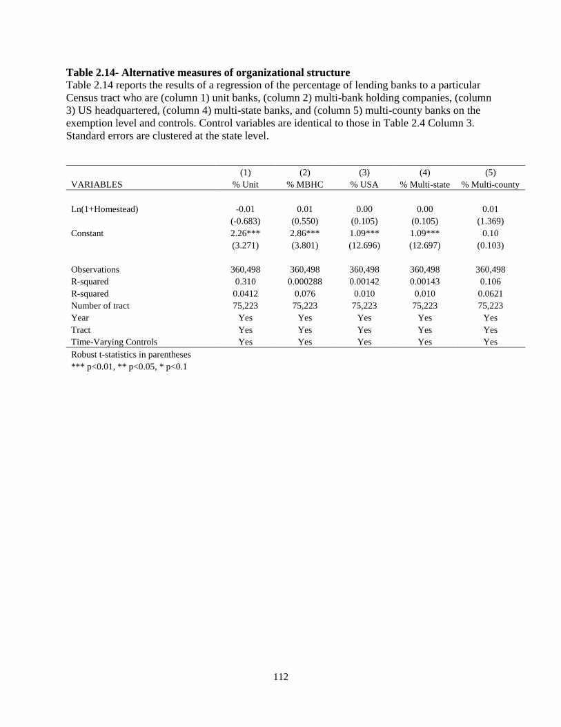
112

Table 2.14- Alternative measures of organizational structure

Table 2.14 reports the results of a regression of the percentage of lending banks to a particular

Census tract who are (column 1) unit banks, (column 2) multi-bank holding companies, (column

3) US headquartered, (column 4) multi-state banks, and (column 5) multi-county banks on the

exemption level and controls. Control variables are identical to those in Table 2.4 Column 3.

Standard errors are clustered at the state level.

(1) (2) (3) (4) (5)

VARIABLES % Unit % MBHC % USA % Multi-state % Multi-county

Ln(1+Homestead) -0.01 0.01 0.00 0.00 0.01

(-0.683) (0.550) (0.105) (0.105) (1.369)

Constant 2.26*** 2.86*** 1.09*** 1.09*** 0.10

(3.271) (3.801) (12.696) (12.697) (0.103)

Observations 360,498 360,498 360,498 360,498 360,498

R-squared 0.310 0.000288 0.00142 0.00143 0.106

R-squared 0.0412 0.076 0.010 0.010 0.0621

Number of tract 75,223 75,223 75,223 75,223 75,223

Year Yes Yes Yes Yes Yes

Tract Yes Yes Yes Yes Yes

Time-Varying Controls Yes Yes Yes Yes Yes

Robust t-statistics in parentheses

*** p<0.01, ** p<0.05, * p<0.1

113

Appendix A:

Variable Definitions

Variable Definition

Ln(1+Homestead)

ln(1+ state homestead exemption). In cases where the federal homestead

exemption level exceeds the state level and state law allows for debtors to

choose between state and federal exemptions, the federal exemption is used.

Homestead exemptions values are also doubled when state law allows.

Unemployment

Rate County unemployment rate. Taken from USA Counties database

Ln(Population) ln(1+ county population). Taken from USA Counties database

Ln(Med. Inc.) ln(1+ county median income). Taken from USA Counties database

House Price

Growth % change in all transactions house price index. Taken from FHFA

Ln(Firm Starts) ln(1+ # of county small business starts). Taken from BEA

Ln(Local

Lenders)

ln(1+ # lenders in local market). Computed from Summary of Deposits data

using branch locations and census tract centroids

HHI

Concentration of local banking market. Computed from Summary of Deposits

data using branch locations and census tract centroids

Small Mkt. Share

Share of local deposits held by banks with less than $1 billion in total assets.

Computed from Summary of Deposits data using branch locations and census

tract centroids

% Large Bank

Branches

Share of local branches owned by banks with greater than $1 billion in total

assets, Computed from Summary of Deposits data using branch locations and

census tract centroids

114

REFERENCES

Adelino, Manuel, Antoinette Schoar, and Felipe Severino. "House Prices, Collateral, and Self-

Employment." Journal of Financial Economics (2015)Web.

Agarwal, Sumit, and Robert Hauswald. "Distance and Private Information in Lending." Review

of Financial Studies (2010): hhq001. Web.

Aghion, Philippe, and Patrick Bolton. "An Incomplete Contracts Approach to Financial

Contracting." The review of economic Studies 59.3 (1992): 473-94. Web.

Alessandrini, Pietro, Manuela Croci, and Alberto Zazzaro. "The geography of banking power:

the role of functional distance*." Banca Nazionale del Lavoro Quarterly Review 58.235

(2005): 129.

Alessandrini, Pietro, Andrea F. Presbitero, and Alberto Zazzaro. "Bank size or distance: what

hampers innovation adoption by SMEs?." Journal of Economic Geography (2009): lbp055.

Barro, Robert J., and Rachel M. McCleary. "Religion and Economic Growth Across Countries."

American Sociological Review (2003): 760-81. Web.

Beck, John H., et al. "Regional Differences in Chapter 13 Filings: Southern Legal Culture Or

Religion?" Review of Social Economy 72.2 (2014): 186-208. Web.

Benmelech, Efraim, and Nittai K. Bergman. "Collateral Pricing." Journal of Financial

Economics 91.3 (2009): 339-60. Web.

Berger, Allen N., Geraldo Cerqueiro, and María F. Penas. "Does Debtor Protection really Protect

Debtors? Evidence from the Small Business Credit Market." Journal of Banking & Finance

35.7 (2011): 1843-57. Web.

Berger, Allen N., and Robert DeYoung. "The effects of geographic expansion on bank

efficiency." Journal of Financial Services Research 19.2-3 (2001): 163-184.

Berger, Allen N., William Goulding, and Tara Rice. "Do Small Businesses Still Prefer

Community Banks?" Journal of Banking & Finance 44 (2014): 264-78. Web.

Berger, Allen N., Leora F. Klapper, and Gregory F. Udell. "The ability of banks to lend to

informationally opaque small businesses." Journal of Banking & Finance 25.12 (2001):

2127-2167.

Berger, Allen N., W. Scott Frame, and Nathan H. Miller. "Credit Scoring and the Availability,

Price, and Risk of Small Business Credit." Journal of Money, Credit, and Banking 37.2

(2005): 191-222.

115

Berger, Allen N., et al. "Does Function Follow Organizational Form? Evidence from the Lending

Practices of Large and Small Banks." Journal of Financial Economics 76.2 (2005): 237-69.

Web.

Berger, Allen N., Richard J. Rosen, and Gregory F. Udell. "Does Market Size Structure Affect

Competition? the Case of Small Business Lending." Journal of Banking & Finance 31.1

(2007): 11-33. Web.

Berger, Allen N., and Gregory F. Udell. "The economics of small business finance: The roles of

private equity and debt markets in the financial growth cycle." Journal of Banking &

Finance 22.6 (1998): 613-673.

Berger, Allen N., and Gregory F. Udell. "Small Business Credit Availability and Relationship

Lending: The Importance of Bank Organisational Structure." The economic journal 112.477

(2002): F32-53. Web.

Berkowitz, Jeremy, and Michelle J. White. "Bankruptcy and small firms' access to

credit." RAND Journal of Economics (2004): 69-84.

Berry, Frances Stokes, and William D. Berry. "State Lottery Adoptions as Policy Innovations:

An Event History Analysis." American political science review 84.02 (1990): 395-415.

Web.

Brevoort, Kenneth P., and Timothy H. Hannan. "Commercial Lending and Distance: Evidence

from Community Reinvestment Act Data." (2004)Web.

Brevoort, Kenneth P., and John D. Wolken. Does Distance Matter in Banking?. Springer, 2009.

Web.

Buckley, Francis H., and Margaret F. Brinig. "Bankruptcy Puzzle, the." J.Legal Stud. 27 (1998):

187. Web.

Cerqueiro, Geraldo, et al. "Debtor Rights, Credit Supply, and Innovation." (2016)Web.

Cerqueiro, Geraldo, and María Fabiana Penas. "How does Personal Bankruptcy Law Affect

Start-Ups?" (2016)Web.

Coval, Joshua D., and Tobias J. Moskowitz. "Home Bias at Home: Local Equity Preference in

Domestic Portfolios." Journal of Finance (1999): 2045-73. Web.

Davydenko, Sergei A., and Julian R. Franks. "Do bankruptcy codes matter? A study of defaults

in France, Germany, and the UK." The Journal of Finance63.2 (2008): 565-608.

Degryse, Hans, and Steven Ongena. "Distance, Lending Relationships, and Competition." The

Journal of Finance 60.1 (2005): 231-66. Web.

116

DeYoung, Robert, Dennis Glennon, and Peter J. Nigro. "Borrower-Lender Distance, Credit

Scoring, and the Performance of Small Business Loans." FDIC Center for Financial

Research Working Paper.2006-04 (2006)Web.

Demirgüç-Kunt, Asli, and Vojislav Maksimovic. "Law, finance, and firm growth."Journal of

finance (1998): 2107-2137.

Djankov, Simeon, Caralee McLiesh, and Andrei Shleifer. "Private credit in 129

countries." Journal of financial Economics 84.2 (2007): 299-329.

Elul, Ronel, and Narayanan Subramanian. "Forum-shopping and personal bankruptcy." Journal

of Financial Services Research 21.3 (2002): 233-255.

Fan, Wei, and Michelle J. White. "Personal Bankruptcy and the Level of Entrepreneurial

Activity." Journal of Law and Economics 46 (2003)Web.

Fay, Scott, Erik Hurst, and Michelle J. White. "The Household Bankruptcy Decision." American

Economic Review (2002): 706-18. Web.

Garmaise, Mark J., and Tobias J. Moskowitz. "Confronting Information Asymmetries: Evidence

from Real Estate Markets." Review of Financial Studies 17.2 (2004): 405-37. Web.

Goodman, Paul. "The Emergence of Homestead Exemption in the United States:

Accommodation and Resistance to the Market Revolution, 1840-1880." The Journal of

American History (1993): 470-98. Web.

Greenstone, Michael, Alexandre Mas, and Hoai-Luu Nguyen. “Do credit market shocks affect

the real economy? Quasi-experimental evidence from the Great Recession and

‘normal’economic times.” No. w20704. National Bureau of Economic Research, 2014.

Gropp, Reint Eberhard, John Karl Scholz, and Michelle J. White. "Personal Bankruptcy and

Credit Supply and Demand." The Quarterly Journal of Economics 112.1 (1997): 217-51.

Web.

Hackney, John. “Debtor protection and small business credit.” University of Washington

Working Paper.

Hart, O., and J. Moore. "A Theory of Debt Based on the Inalienability of Human Capital."

Quarterly Journal of Economics 109.4 (1994): 841-79. Web.

Hart, Oliver, and John Moore. "Default and Renegotiation: A Dynamic Model of Debt."

Quarterly Journal of Economics (1998): 1-41. Web.

Hart, Oliver. Firms, Contracts, and Financial Structure. Oxford university press, 1995. Web.

117

Hau, Harald. "Location Matters: An Examination of Trading Profits." Journal of Finance (2001):

1959-83. Web.

Hauswald, Robert, and Robert Marquez. "Competition and Strategic Information Acquisition in

Credit Markets." Review of Financial Studies 19.3 (2006): 967-1000. Web.

Hynes, Richard M., Anup Malani, and Eric A. Posner. "The Political Economy of Property

Exemption Laws*." Journal of Law and Economics 47.1 (2004): 19-43. Web.

Heider, Florian, and Alexander Ljungqvist. "As certain as debt and taxes: Estimating the tax

sensitivity of leverage from state tax changes." Journal of Financial Economics 118.3

(2015): 684-712.

Kennickell, Arthur B. "Using Income Data to Predict Wealth." Federal Reserve Board.Retrieved

on April 22 (1999): 2005. Web.

King, Robert G., and Ross Levine. "Finance and growth: Schumpeter might be right." The

quarterly journal of economics (1993): 717-737.

Kumar, Alok, Jeremy K. Page, and Oliver G. Spalt. "Religious Beliefs, Gambling Attitudes, and

Financial Market Outcomes." Journal of Financial Economics 102.3 (2011): 671-708. Web.

Kumar, Alok. "Who Gambles in the Stock Market?" The Journal of Finance 64.4 (2009): 1889-

933. Web.

La Porta, Rafael, et al. "Legal determinants of external finance." Journal of finance (1997): 1131-

1150.

Levine, Ross. "Financial development and economic growth: views and agenda." Journal of

economic literature (1997): 688-726.

Martin, Robert, and Bruce Yandle. "State Lotteries as Duopoly Transfer Mechanisms." Public

Choice 64.3 (1990): 253-64. Web.

Petersen, Mitchell A., and Raghuram G. Rajan. "The Benefits of Lending Relationships:

Evidence from Small Business Data." The journal of finance 49.1 (1994): 3-37. Web.

---. "Does Distance Still Matter? the Information Revolution in Small Business Lending." The

Journal of Finance 57.6 (2002): 2533-70. Web.

Rajan, Raghuram G., and Luigi Zingales. Financial dependence and growth. No. w5758.

National bureau of economic research, 1996.

Schumpeter, Joseph Alois. The theory of economic development: An inquiry into profits, capital,

credit, interest, and the business cycle. Vol. 55. Transaction publishers, 1934.

118

Severino, Felipe, Meta Brown, and Brandi Coates. "Personal bankruptcy protection and

household debt." Available at SSRN 2447687 (2014).

Stein, Jeremy C. "Information Production and Capital Allocation: Decentralized Versus

Hierarchical Firms." Journal of Finance 57.5 (2002): 1891-921. Web.

Stiglitz, Joseph E., and Andrew Weiss. "Credit Rationing in Markets with Imperfect

Information." The American Economic Review (1981): 393-410. Web.

Stulz, RenéM, and Herb Johnson. "An Analysis of Secured Debt." Journal of Financial

Economics 14.4 (1985): 501-21. Web.

Sullivan, Teresa A., Elizabeth Warren, and Jay Lawrence Westbrook. "As we Forgive our

Debtors." New York (1989)Web.

Udell, Gregory F. "Loan quality, commercial loan review and loan officer contracting." Journal

of Banking & Finance 13.3 (1989): 367-382.

Vig, Vikrant. "Access to collateral and corporate debt structure: Evidence from a natural

experiment." The Journal of Finance 68.3 (2013): 881-928.

Vincenty, Thaddeus. "Direct and Inverse Solutions of Geodesics on the Ellipsoid with

Application of Nested Equations." Survey review 23.176 (1975): 88-93. Web.

White, Michelle J. "Why Don't More Households File for Bankruptcy?" Journal of Law,

Economics, & Organization (1998): 205-31. Web.

---. "Why it Pays to File for Bankruptcy: A Critical Look at the Incentives Under US Personal

Bankruptcy Law and a Proposal for Change." The University of Chicago Law Review

(1998): 685-732. Web.

---. "Corporate and Personal Bankruptcy Law." Annu.Rev.Law Soc.Sci 7 (2011): 139-64. Web.