cjoita/imar/tbarbu-teza_abilitare.pdf · 2017-02-07 · 3 contents (a) summary...
TRANSCRIPT

ROMANIAN ACADEMY
Speech and Image Processing and Analysis Models
Applied to Biometrics and Computer Vision
Habilitation Thesis
TUDOR BARBU
Senior Researcher I
Institute of Computer Science of the Romanian Academy
Iaşi, Romania
February, 2015

2
Familiei mele,
3
CONTENTS
(a) Summary ……………………………………………………………………………………...5
Rezumat ……………………………………………………………………………………....7
(b) Scientific achievements and career development plans ……………………………………....9
(i) Scientific and professional achievements ………………………………………………….9
1. Mathematical models for image processing and machine learning …………………….10
1.1. Image filtering methods using hyperbolic second-order equations ……………….10
1.2. Nonlinear diffusion based image noise removal approaches………………………13
1.2.1. Related work..…………………………………………………………………...13
1.2.2. Novel anisotropic diffusion models for image restoration….….……………….15
1.2.3. Image denoising approach based on diffusion porous media flow ……………..19
1.2.4. Fourth order diffusion models for image noise reduction…………….....……....23
1.3. Variational PDE techniques for image denoising and restoration.………………...25
1.3.1. A robust variational PDE model for image denoising………………………......25
1.3.2. Variational image restoration approach………………………….……………...28
1.4. Mathematical models for media feature vector classifiers and metrics……….……31
1.4.1. A Hausdorff-derived metric for different-sized 2D feature vectors……….……31
1.4.2. A special metric for complex feature vectors…………………………………...33
1.4.3. Automatic unsupervised classification algorithm…..……………………………35
1.4.4. Automatic clustering models based on validity indexes………….……………..36
1.5. Conclusions…………..…………………………………………………………….38
2. Biometric authentication techniques………………………………………………….…40
2.1. Voice recognition approaches using mel-cepstral analysis………………………..41
2.1.1. MFCC-based speech feature extraction solutions……………………..……….41
2.1.2. Supervised text-dependent voice recognition technique…………….…………42
2.1.3. Automatic unsupervised speaker classification model……….………………...47
2.2. Robust face recognition techniques………………………………………………..50
2.2.1. Eigenimage-based face recognition approach using gradient covariance……...50
2.2.2. Face recognition technique using 2D Gabor filtering………………….……....57
2.2.3. Automatic unsupervised face recognition system………………………..….…61
2.3. Person authentication via fingerprint recognition…………………...……………..64
2.3.1. Minutiae-based fingerprint authentication approach…………………………..65
2.3.2. Fingerprint pattern matching using 2D Gabor filtering………….…………….68
2.3.3. Pattern-based fingerprint recognition using 2D Wavelet Decomposition……..70
2.4. Multi-modal biometric technologies……………………………………………….73
2.5. Conclusions……………………………………………………….………………..76

4
3. Image analysis based computer vision models………………………………………….78
3.1. Novel image segmentation techniques………………………………………..……..78
3.1.1. Automatic region-based image segmentation methods………………………....79
3.1.2. Level set based contour tracking model………………………………..……….82
3.2. Temporal video segmentation approaches…………………………………….…….85
3.2.1. Histogram comparison based shot detection techniques…………..……………86
3.2.2. Automatic feature-based video cut identification model……….……………….87
3.3. Variational PDE models for image reconstruction……………..…………….……..93
3.4. Image and video recognition methods……………………………..………………..97
3.4.1. Automatic image recognition techniques……………………………………….97
3.4.2. Video sequence recognition approach…………………………………………103
3.4.3. Image and video object recognition models…………...………………………106
3.5. Content-based image indexing and retrieval systems…………………….…….….110
3.5.1. Content-based image indexing models……….…………..……………………110
3.5.2. Content-based image retrieval techniques……………………………..………113
3.6. Image and video object detection and tracking solutions………………………….121
3.6.1. Automatic image object detection techniques………………………...……….121
3.6.2. Video object detection approaches………………………………….…………133
3.6.3. Video tracking methods………………………………………………………..137
3.7. Conclusions………………………………………………………………………...145
(ii) Professional, scientific and academic career evolvement and development plans……....146
(iii) References…………………………………………………………………..…………...153
5
(a) Summary This abilitation thesis presents the most significant scientific accomplishments I have
achieved since I received the PhD degree in January 2005, and also my future professional,
scientific and academic career development and evolvement plans. Besides this summary, it is
composed of a main part b, containing three subparts.
The major subpart b(i), entitled Scientific and professional achievements, describes in
three chapters the most important results obtained in the period 2005-2014. In these almost ten
years my research activity has lied at the intersection of computer science, digital signal
processing, and applied mathematics. I have essentially followed four main research directions in
this period: image pre-processing, machine learning, biometrics and computer vision.
Mathematical models, mostly based on partial differential equations (PDEs), have been
introduced in all these domains. Since the most important of these domains, which are biometrics
and computer vision, are mainly based on image and voice signal analysis, many speech and
image analysis techniques for biometrics and computer vision have been developed by us. The
other two approached domains have the role to facilitate the tasks related to biometrics and
computer vision. The proposed image pre-processing techniques are based on PDE models and
enhance the images, thus facilitating the potential image analysis tasks. The machine learning
algorithms are widely used in both biometrics and computer vision. Our machine learning
solutions represent novel media feature vector classification algorithms using some specially
created metrics. Each chapter is composed of several sections, each section being related to a
subdomain and composed of subsections corresponding to various techniques, ending with a
conclusion section.
First chapter, entitled Mathematical models for image processing and machine learning, is
related to my first two directions. In the first section there are described our proposed image
filtering methods using hyperbolic second-order equations. The developed image noise reduction
approaches based on nonlinear diffusion are presented in the second section. The third section
describes the proposed variational PDE image denoising and restoration techniques. Some
special metrics for media (audio, image and video) feature vectors and several automatic feature
vector clustering techniques modeled by us are explained in the fourth section.
Second chapter, entitled Biometric authentication techniques, describes our main results
achieved in the biometrics domain. The developed voice recognition techniques based on mel-
cepstral speech analysis are discussed in the first section. The second section presents the
proposed facial recognition models, while the third section presents our fingerprint
authentication approaches. The investigated multi-modal biometric technologies are described in
the fourth section.
The third chapter is entitled Image analysis based computer vision models and presents my
accomplishments in computer vision area. Its first section describes the proposed image
segmentation techniques, while our temporal video segmentation approaches are described in the
second section. The third section presents the variational PDE-based image reconstruction
models introduced by us. The considered image and video recognition solutions are discussed in
the fourth section. In the fifth section there are described content-based image indexing and
retrieval systems. The developed image and video object detection and tracking technologies are
outlined in the sixth section.
All research results described in these chapters have been soft-implemented, and
disseminated in numerous publications. Since January 2005, I have authored over 66 published

6
works disseminating the major achievements in the mentioned domains, including 2 books, 1
book chapter, 33 articles published in recognized international journals (18 ISI journals and 15
journals indexed by international databases) and 30 papers published in volumes of international
scientific events (including 2 conferences ranked as A, 5 ranked as B, 3 ranked as C, by ARC).
Besides these works, the research results have been disseminated in 20 scientific reports
elaborated at our institute, under my coordination. The scientific impact of my works is also
proven by the 160 citations (no self-citations) received by them, according to Google-Academic.
The second subpart b(ii), entitled Professional, scientific and academic career
evolvement and development plans, disscuses the future research results, first. In the future I
will continue to follow the mentioned research directions, improving the proposed techniques,
developing new methods and approaching new subdomains. In b(ii) I suggest how our existing
approaches can be further improved, and how new image restoration, biometric authentication
and computer vision solutions would look like. Several new PDE models for denoising and
inpainting are mainly discussed. New subdomains of the major domains will also be considered.
In b(ii) I explain how new biometrics subdomains, such as iris recognition and text-independent
voice recognition, or new computer vision areas, like image registration and optical flow, will be
approached as part of my future research.
Then, my academic career evolvement and development plans are outlined. I consider and
explain in detail the following major objectives of the career development plan: forming a new
generation of well-prepared researchers in my domains of interest; building and coordinating
effective research collectives capable to conduct important projects; establishing more scientific
collaborations with well-known researchers and institutes from Romania or abroad; performing
teaching activities.
My abilitation thesis ends with the bibliography b(iii), where references of top 10 selected
papers are marked in bold.

7
(a) Rezumat
Această teză de abilitare prezintă cele mai importante dintre realizările mele ştiinţifice
obţinute de la primirea titlulul de doctor, în ianuarie 2005, până în prezent, şi de asemenea
planurile de dezvoltare şi evoluţie a carierei mele profesionale, ştiinţifice şi academice. Pe lângă
acest rezumat, teza este compusă dintr-o parte principală b, conţinând trei subpărţi.
Subpartea principală b(i), intitulată Realizări ştiinţifice şi profesionale, descrie în cele trei
capitole ale sale cele mai importante rezultate obţinute în perioada 2005-2014. În aceşti aproape
zece ani, activitatea mea de cercetare s-a situat la intersecţia dintre informatică, procesarea
semnalelor digitale şi matematica aplicată. În respectiva perioadă am urmat în principal
următoarele patru direcţii de cercetare: pre-procesarea imaginilor, învăţare automată, biometrie şi
vizune computerizată. Modele matematice, în majoritate bazate pe ecuaţii cu derivate parţiale, au
fost introduse în toate aceste domenii. Deoarece cele mai importante dintre aceste domenii, şi
anume biometria şi viziunea computerizată, sunt bazate mai ales pe analiza semnalului de
imagine şi voce, numeroase tehnici de analiză a vorbirii şi imaginilor, utilizabile în biometrie şi
viziunea computerizată, au fost dezvoltate de către noi. Celelalte două domenii abordate au rolul
de a facilita procesele biometrice sau ale viziunii computerizate. Tehnicile de pre-procesare a
imaginilor pe care le-am propus sunt bazate pe modele PDE şi prin îmbunătăţirea imaginilor
facilitează potenţialele procese de analiză imagistică. Algoritmii de învăţare automată sunt des
utilizaţi atât în biometrie, cât şi în viziunea computerizată. Soluţiile noastre de învăţare automată
reprezintă noi algoritmi de clasificare a vectorilor de trăsături media, care utilizează metrici
special construite. Fiecare capitol este compus din câteva secţiuni, fiecare secţiune abordând un
anumit subdomeniu şi compusă la rândul său din subsecţiuni corespunzând unor diverse tehnici,
şi se încheie cu concluzii.
Primul capitol, intitulat Modele matematice de procesare a imaginilor şi învăţare
automată, se referă la primele două direcţii. În prima secţiune sunt descrise metodele propuse
pentru filtrarea imaginilor utilizând ecuaţii hiperbolice de ordinul II. Tehnicile de reducere a
zgomotului din imagine bazate pe difuzia neliniară, dezvoltate de noi, sunt prezentate în
secţiunea a doua. Cea de-a treia secţiune prezintă tehnicile PDE variaţionale propuse pentru
curăţirea de zgomot şi restaurarea imaginilor. Metricile speciale pentru vectorii de trăsături
media (audio, imagistici și video) şi tehnicile automate de clusterizare automată a vectorilor de
trăsături, pe care le-am modelat, sunt explicate în secţiunea a patra.
Al doilea capitol, intitulat Tehnici de autentificare biometrică, descrie cele mai importante
rezultate pe care le-am obţinut în domeniul biometric. Tehnicile dezvoltate pentru recunoaşterea
vocii, bazate pe analiza mel-cepstrală a vorbirii, sunt discutate în prima secţiune. Cea de a doua
descrie modelele de recunoaştere facială propuse, iar a treia secţiune prezintă metodele noastre
de autentificare a amprentelor digitale. Tehnologiile biometrice multi-modale investigate sunt
descrise în cea de-a patra secţiune.
Capitolul trei este intitulat Modele de viziune computerizată bazate pe analiza imagistică
şi prezintă rezultatele obţinute în domeniul viziunii computerizate. Prima secţiune descrie
tehnicile de segmentare a imaginii propuse, în timp ce metodele noastre de segmentare temporală
video sunt descrise în a doua secţiune. A treia secţiune prezintă modelele variaţionale de tip PDE
pentru reconstrucţia imaginilor, pe care le-am introdus. Soluţiile considerate pentru recunoaştere
a imaginilor şi secvenţelor video sunt discutate în a patra secţiune. În secţiunea cinci sunt
descrise sisteme informatice de indexare și regăsire de imagini pe baza de conţinut. Tehnologiile

8
construite pentru detectarea şi urmărirea obiectelor imagistice şi video sunt prezentate în
secţiunea a şasea.
Rezultatele cercetării descrise în aceste capitole au fost implementate soft, și diseminate în
numeroase publicaţii. Începând cu ianuarie 2005, am publicat peste 66 de lucrări diseminând
principalele realizări în domeniile menţionate, incluzând 2 cărţi, 1 capitol de carte, 33 articole
publicate în jurnale internaţionale recunoscute (18 jurnale ISI şi 15 jurnale indexate de bazele de
date internaţionale) şi 30 articole publicate în volume ale evenimentelor ştiinţifice internaţionale
(incluzând 2 conferinţe tip A, 5 de tip B, 3 de tip C, conform ARC). Înafara acestor lucrări,
rezultatele cercetării au fost diseminate în 20 de rapoarte ştiinţifice elaborate la institutul nostru,
sub coordonarea mea. Impactul ştiinţific ridicat al acestor lucrări este demonstrat de cele 160
citări (excluzând auto-citările) primite, conform Google-Academic.
Cea de-a doua subparte b(ii), intitulată Planuri de dezvoltare şi evoluţie a carierei
profesionale, ştiinţifice şi academice, ia mai întâi în discuţie viitoarele rezultate în cercetare. În
viitor voi continua să urmez direcţiile de cercetare menţionate, îmbunătăţind technicile propuse,
dezvoltând noi metode şi abordând noi subdomenii. În b(ii) sunt sugerate modalităţile prin care
metodele noastre existente pot fi îmbunătăţite, precum şi modul în care vor arăta noile soluţii de
restaurare imagistică, autentificare biometrică şi viziune computerizată. Câteva modele noi de tip
PDE pentru filtrare şi reconstrucţie sunt în principal abordate. Totodată, noi subdomenii ale
domeniilor principale vor fi considerate. În b(ii) sunt apoi explicate modalităţile de abordare în
cadrul cercetării viitoare ale subdomeniilor nou-introduse, precum recunoaşterea irisului ori
recunoaşterea vocii independentă de text, în cazul biometriei, sau înregistrarea imaginilor şi
fluxul optic, în cazul viziunii computerizate.
În continuare sunt prezentate planurile de evoluţie şi dezvoltare ale carierei academice.
Am considerat şi explicat în detaliu următoarele obiective majore ale planului de dezvoltare a
carierei: formarea unei noi generaţii de cercetători bine pregătiţi în domeniile mele de interes;
organizarea şi coordonarea unor colective de cercetare eficiente, capabile să ducă la îndeplinire
proiecte importante; stabilirea de noi colaborări ştiinţifice cu personalităţi şi instituţii de renume
în cercetare; desfăşurarea unor activităţi didactice, de predare.
Teza de abilitare se încheie cu bibliografia b(iii), în care referințele lucrărilor selectate în
top 10 sunt marcate in bold.
9
(b) Scientific achievements and career development plans
(i) Scientific and professional achievements
This main part of the abilitation thesis presents the most important scientific results
accomplished in the last 10 years that is the period following my PhD award. It is composed of 3
chapters, each of them describing the major achievements in one of these main areas of interest:
image enhancement, biometrics and computer vision. Besides the proposed PDE-based image
denoising and restoration models, first chapter outlines also some machine learning algorithms.
The most significant results achieved in the biometrics field are described in the second chapter,
where both supervised and unsupervised biometric recognition models, based on voice, face,
fingerprints and combinations of these identifiers, are presented. The third chapter illustrates the
main computer vision achievements, representing original image and video segmentation, image
reconstruction, image and object recognition, CBIR and object detection/tracking techniques. My
major contributions to the approached domains, described in the next 3 chapters, are as follows:
A linear PDE-based image denoising technique using hyperbolic second-order equations
A nonlinear anisotropic diffusion model for image restoration
Image noise removal approach based on diffusion porous media flow
A 4th-order diffusion-based model for image noise reduction
Two novel PDE variational models for image denoising
A Hausdorff-Pompeiu derived metric for different-sized 2D feature vectors
A novel similarity metric constructed for images characterized by key points
Automatic unsupervised classification models using region-growing and validation indexes
Text-dependent voice recognition system using a robust DDMFCC-based feature extraction
An automatic unsupervised speaker recognition model
An eigenimage-based facial recognition technique
A 2D Gabor filtering-based face recognition approach
A SIFT-based automatic unsupervised face recognition model
Minutia-matching based fingerprint recognition solution
Pattern-based fingerprint matching methods using 2D Gabor filters and DWT decomposition
Multimodal biometric technologies combining voice, face and fingerprint recognition models
Automatic moment-based image segmentation techniques
A PDE level-set based contour tracking model
An automatic temporal video segmentation technique
A robust PDE variational image reconstruction approach
Novel image and video recognition models using various content-based feature vectors
Object recognition model using moment-based shape analysis and content-based recognition
Automatic clustering-based image indexing and retrieval techniques
Content-based image retrieval systems using SAM indexing and relevance-feedback schemes
Automatic face detection technique based on skin filtering and cross-correlation procedures
A SVM-based human cell detection technique using HOG-based feature vectors
Object detection and tracking models using temporal-differencing and object matching
Video tracking technique using a novel N-Step Search algorithm and HOG features.
The results described in these chapters have been disseminated in over 66 published works
(books, chapters, articles in recognized international journals or conference volumes). My
selected most relevant 10 papers contain the most accomplishments from the above list.
10
1. Mathematical models for image processing and machine learning
During the past three decades, the mathematical models have been increasingly used in
some traditionally engineering domains like signal and image processing, analysis, and computer
vision. This chapter describes several robust mathematical models for image pre-processing
(processing images for future analysis tasks) and machine learning.
The most important image pre-processing tasks, namely the image denoising and
restoration, are performed using some partial differential equation (PDE) based mathematical
models. The partial differential equations have been successful for solving various image
processing and computer vision tasks since 1980s [1]. The variational and PDE-based
approaches have been widely used and studied in these domains in the last decades, mainly
because of their modeling flexibility and some advantages of their numerical implementation [1].
Image noise reduction with feature preservation is still a focus in the image processing
field and a serious challenge for the researchers. An efficient denoising technique has to not only
substantially reduce the quantity of image noise but also preserve the image boundaries and other
characteristics. The conventional smoothing models, such as the averaging, median, Wiener, or
the classic 2D Gaussian filter succeed in noise reduction, but could also have undesired effects
on edges or other image details and structures [2,3]. The PDE-based models provide efficient
image filtering while preserving the features [4].
Some novel linear and nonlinear PDE-based image noise removal techniques are described
in the next three sections. Thus, a modified Gaussian filter kernel provided by second-order
hyperbolic diffusion equations is introduced in section 1.1. Several nonlinear diffusion equation
based filtering techniques are discussed in the second section. The third section describes our
PDE variational image restoration models.
Several mathematical models are introduced for the classification of various media feature
vectors. Supervised and unsupervised classification models are described in the fourth section,
related to machine learning. Some metrics specially created for complex feature vectors and used
by these classifiers, are also modeled mathematically and presented in 1.4.
1.1 . Image filtering methods using hyperbolic second-order equations
Gaussian noise, representing the statistical noise having the probability density function
equal to that of the normal distribution is very often encountered in acquired digital images. So,
the Gaussian noise reduction represents a very important image processing task that has been
approached using both linear and nonlinear filtering algorithms [2,3].
Many classical image processing techniques can be reinterpreted as approximations of
PDE-based models. Thus, the classic 2D Gaussian filtering model can be provided by the heat
equation. This Gaussian filter, like other conventional linear filters such as the average filter [2],
is efficient in smoothing the noise, but also has the disadvantage of blurring image edges. For
this reason, I proposed a linear PDE-based denoising model using a modified Gaussian filter
kernel in a 2012 paper [5].
The introduced mathematical model differs from the classic Gaussian model provided by
heat equations, by a localization property. The classical filter has no localization property, the
heat equation solution propagating with infinite speed, and this fact affects the edges. The
11
classical Gaussian kernel, 0,,,4
1, 24
22
tRyxet
yxG t
yx
t
, is replaced with a modified
kernel provided by some second-order hyperbolic equations [5]. The new improved kernel,
RRyxtE 2,0:,, , is obtained as the solution of the following PDE hyperbolic
model:
2
2
22
, 0, ,
0,,0 ,,,0
0
Ryxt
yxt
EyxE
Et
E
t
E
(1.1)
where 0 , 0 and is the Dirac measure in 2R concentrated in 0. Therefore, the Gaussian
restoration process ),)(*(),,( 0 yxuGyxtu t becomes:
2),(),,(),)(*)((),,( 00
RdduyxtEyxutEyxtu (1.2)
where 2
00 ),( ),,( Ryxyxuu is the image affected by noise, while u represents the
restored image and is also the solution to the second-order linear differential equation:
2
0
2
2
22
,,0),,0(,,,,0
0,in ,0
Ryxyxt
uyxuyxu
Rut
u
t
u
(1.3)
This equation, representing the telegraphist’s equation, is used also as a non-Fourier
model for heat propagation (the Cattaneo-Vernotte model). It is well known that the solution u to
(1.3) propagates with finite speed [6], and so, taking (1.3) as a model for image denoising, it
behaves better than the standard Gaussian model. A robust mathematical treatment of the
proposed restoration model is also provided. We have demonstrated in [5] the existence and
uniqueness of the hyperbolic equation’s solution. The equation (1.3) has a unique weak solution
u = u (t, x, y) which is continuous in t with values in )( 22 RL .
The described PDE hyperbolic model is approximated in [5] using an implicit finite
difference scheme. The following numerical approximation scheme has been provided in our
paper:
02 1212212 kkkk Auhuuhuh (1.4)
where h > 0 and A is the elliptic operator uAu .
The convergence of the numerical scheme given by (1.4) is also demonstrated in [5]. For
simplicity, the following explicit scheme can be used instead of it:
12
,...2,1 ,02 1
2
2
2
2
2
21
kAu
hu
h
hAu
h
hu kkkk
(1.5)
This scheme converges to a solution representing the restored image u in a low number of
iterations. Our iterative smoothing algorithm not only removes a great amount of Gaussian noise
from the image, but also preserves the image edges very well. It has been tested on hundreds
images corrupted with various levels of Gaussian noise, very good denoising results being
obtained [5]. Also, our PDE restoration technique outperforms most classical image filtering
algorithms, as resulting from the performed method comparisons. Such a method comparison is
described in the next figure.
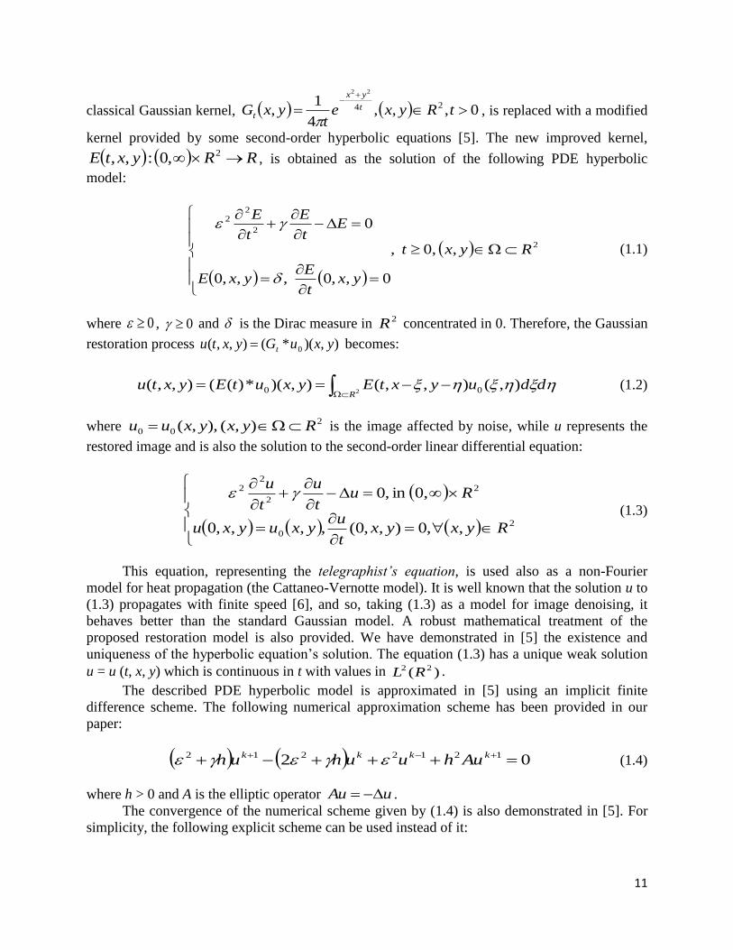
Fig. 1.1. The modified Gaussian filter compared with some conventional filters
One can see in Fig. 1.1 the original grayscale Lena image (a), the image affected by
Gaussian noise characterized by a standard deviation value of 0.5 (b), the smoothing result
obtained by a [3 × 3] 2D Gaussian filter kernel (c), the averaging filtering result produced by a [3
× 3] mean filter kernel (d) and, finally, the image filtered by our modified Gaussian model. The

13
improved Gaussian filter substantially increases image quality. It not only removes a greater
amount of noise than the classic Gaussian kernel and also provides a better image contrast. Also,
this hyperbolic denoising procedure executes very fast, being characterized by a low complexity
and computational time [5].
Also, the linear PDE-based model described here can be further transformed into more
sophisticated nonlinear diffusion schemes [5]. Such a nonlinear hyperbolic filtering model,
which makes the focus of our current research, has the following form:
yx
yxtyxtu
yxuyxt
u
yxuyxu
uuuudivt
u
t
uu
, ,
, ,0 ,0,,
,,,0
,,,0
0
1
0
0
2
2
2
(1.6)
Other nonlinear 2nd and 4th order hyperbolic diffusion models derived from (1.3) are also
considered. It should be said also that PDE hyperbolic model (1.3) can be used as a filtering
technique to extract the coherent and incoherent components of a forced turbulent flow and to
identify coherent vortices as in [7]. We expect to give more details in a forthcoming article.
1.2. Nonlinear diffusion based image noise removal approaches
The diffusion equations have proved their usefulness in domains like physics and
engineering sciences for a very long time. Since 1980s, these PDEs have played an important
role in the image processing and analysis domains [1]. Diffusion equations offer numerous
advantages for image denoising and restoration [8]. They are the mathematically best-founded
approaches in image pre-processing. Also, they allow a reinterpretation of some classical
filtering techniques under a new unifying framework. Thus, the idea of using the diffusion
equations in image denoising and restoration arose from the use of the classic Gaussian filter in
multiscale image analysis. The convolution of an image with a 2D Gaussian kernel amounts to
solve the diffusion equation in two dimensions (heat equation).
A diffusion equation having the form utyxCdivt
u
),,( becomes linear if the
diffusion tensor C does not depend on the evolving image u (t, x, y). The linear diffusion models
are the simplest PDE–based image denoising techniques. The main drawback of the linear PDE
denoising algorithms is the blurring effect that can affect image details. The linear diffusion has
no localization property and may dislocate image boundaries when moving from finer to coarser
scales. The nonlinear diffusion is characterized by a tensor that is a function of the image u:
yxtugtyxC ,,),,( . The nonlinear diffusion based techniques overcome the blurring and
localization problems faced by the linear approaches [8]. They perform the image smoothing
along but not across the edges.
1.2.1. Related work
These nonlinear PDE models have been extensively studied since the early work of P.
Perona and J. Malik in 1987 [9]. The influential Perona-Malik denoising scheme represents the

14
most popular nonlinear anisotropic diffusion technique. If the diffusion tensor is constant over
the entire image domain, one speaks of isotropic diffusion, while a space-dependent filtering is
called anisotropic. The filter proposed by Perona and Malik reduces the diffusivity at those
locations having a larger likelihood to represent image edges and is characterized by the
following nonlinear diffusion equation:
uugdivt
uu t
)(
2 (1.7)
with the noisy image 0u as the initial condition. Perona and Malik considered two variants of the
monotonous decreasing diffusivity function that controls the blurring intensity, ,0,0:g ,
which are:
2
22
1
1)( ;)(
2
2
k
ssgesg k
s
(1.8)
where parameter k > 0 represents the diffusivity conductance [9]. They discretized the PDE model
as following:
t
W
t
W
t
E
t
E
t
S
t
S
t
N
t
N
tt ucucucucuu 1 (1.9)
where
yxt
yxtt
Wyxt
yxtt
Eyxt
yxtt
Syxt
yxtt
N uuuuuuuuuuuu ,,1,1,1,,1,,1 ,- , ,- (1.10)
and
t
W
t
W
t
E
t
E
t
S
t
S
t
N
t
N ugcugcugcugc ,,, (1.11)
Perona-Malik scheme provides an efficient edge-preserving image smoothing that has
been further improved in many nonlinear diffusion based techniques derived from it in the recent
years. There are numerous papers that investigate the mathematical properties, the numerical
implementations and the possible applications of this denoising framework. The stability of
Perona-Malik model has been extensively studied in the last two decades [8,10]. The nonlinear
PDE-based techniques inspired by the influential Perona-Malik scheme differ from each other
through the diffusivity (edge-stopping) function. The function g has to satisfy some certain
conditions, such as positivity, decreasing monotony, g (0) = 1 and convergence to 0.
The total variation (TV) diffusivity, given by s
sg1
)( 2 , and its regularized version
22
2 1)(
ssg represent popular edge-stopping functions [11]. Charbonnier et al. proposed

15
the Charbonnier diffusivity [12], that is
2/1
2
22 1)(
k
ssg , and J. Weickert [8] proposed an
anisotropic diffusion model based on edge-stopping function
0 if ,1
0 if ,1)()/(2
22
s
sesgm
m
ks
C
,
where )2 1(1 mCe m
Cm , 4,3,2m , 3366.22 C , 9183.23 C and 3148.34 C . Black et al.
developed the robust anisotropic diffusion (RAD) [13]. They used robust estimation theory to
model the diffusivity function called Tukey’s biweight:
5 if ,0
5 if ,
51
)(
22
22
2
2
2
2
ks
ks
k
s
sg.
These nonlinear diffusion techniques may also differ through the way they choose the
diffusivity conductance parameter. When the gradient magnitude exceeds the value of k, the
corresponding boundary is enhanced. Some methods, including the Perona-Malik filter, use a
fixed k value. Other approaches make this parameter a function of time, k (t). A high k (0) value
is considered at the beginning, then k (t) is reduced gradually, as the image is smoothed. Other
approaches detect automatically this parameter as a function of the current state of the evolving
image. Various noise estimation methods can be used in the detection process [14]. A solution is
to estimate the noise at each iteration as the difference between the averages of images processed
by the morphological operations of opening and closing. In this case the conductance parameter
is computed as SuavgSuavgk - , S being a structuring element. Another solution is
to estimate the noise using the p-norm of the image: m
uk
p
, where m is the number of
pixels and is proportional to the average intensity [14]. Other solutions determine the
conductance diffusivity as the robust scale of the image, by using statistics like the median [13]:
uumedianuumediank e )()(4826.1 .
1.2.2. Novel anisotropic diffusion models for image restoration
We developed a nonlinear anisotropic diffusion-based restoration technique that improves
the Perona-Malik denoising scheme and outperforms the other nonlinear PDE based smoothing
algorithms [15,16]. It is based on the following PDE parabolic model:
yx
uyxu
uugdivt
uuK , ,
,,0 0
2
)( (1.12)
where 0u is the initial (noised) state of the image and 2R represents its domain. The
nonlinear diffusion equation provided by (1.12) uses a novel edge-stopping function
,0,0:)(uKg that is modeled as following:
16
0 if ,1
0 if ,)(
)( 22
)(
s
ss
uK
sg uK
(1.13)
where the parameters 8.0 ,5.0, and 5 ,5.0 . The function given by (1.13) is based
on a conductance diffusivity parameter that depends on the current state of the image. We
compute automatically this parameter in [15], on the basis of image noise estimation at each time
t, as following:
)(
)(F
uun
umedianuK
, (1.14)
where 1 ,0 , F
u is the Frobenius norm of image u, median(u) represents its median value
and n(u) is the number of its pixels.
Then we demonstrate that the proposed diffusivity function is properly modeled, satisfying
the conditions required by an edge-stopping function. We have 1)0()( uKg . Also, function
)(uKg is always positive, because . ,0
)(2
Rss
uK
It is also monotonically
decreasing, because )()()(
)( 2
2)(2
2
2
1
2
1)( sgs
uK
s
uKsg uKuK
,
21 ss
, Also, we have 0 )(lim 2
)(
sg uKs
[16].
The proposed edge-stopping function has also an important property related to the flux. If
one considers the flux function defined as )( 2
)( sgss uK , the image enhancement and edge
sharpening process depends on the sign of its derivative, s' [17]. Thus, if the derivative of
the flux function of a diffusion model is positive ( 0' s ), then that model is a forward
parabolic equation. Otherwise, for 0' s , that nonlinear diffusion model represents a
backward parabolic equation [15-17]. The derivative of the flux function of our PDE model is
computed as following:
22
2
2
2
)(
22
)(
)()( )('2)()('
ss
suK
s
uKsgssgs uKuK (1.15)
which leads to
2/32
22
2/3222
2
2
)()()('
)()()('
s
uKss
s
uKs
ss
suK
s
uKs (1.16)
17
Since
ss
uK
,0
)(2/32
one obtains 0' s for any s, which means our PDE
denoising model is a forward parabolic equation that is stabile and quite likely to have a solution.
We investigated the existence of this solution in the first selected paper (see Barbu &
Favini [16]), where we provide a rigorous mathematical treatment for our anisotropic diffusion-
based model. While, in general, the problem (1.12) is ill-posed, we have proved the existence
and uniqueness of a weak solution in a certain case that is related to some values of the model’s
parameters. We have demonstrated that our nonlinear PDE model converges if 2 . The
following modification of the edge-stopping function has been considered:
2
2
( )
( )if 0
( )
if 0
K u
K us M
sg s
s
(1.17)
where 0M is arbitarily large but fixed. If the parabolic model (1.12) uses )(uKg given by
(1.17) for each 2
0( )u L (the space of all Lebesgue square integrable functions on ) there
is a unique weak solution u to the PDE problem (see [16]).
The proposed nonlinear anisotropic diffusion model was discretized using a 4-nearest-
neighbours discretization of the Laplacian operator. So, from the equation (1.12) one obtains
uuguugtyxutyxuuugdivt
uuKuKuK
)(
2
)(
2
)( ,,1,, ,
which leads to the next numerical approximating scheme:
pNq
qpqpuK
tt tutuguu )()( ,
2
,)(
1 (1.18)
where 1 ,0 , pN is the set of pixels representing the 4-neighborhood of the pixel p (given by
pair of coordinates x, y) and ),(),()(, tputqutu qp is the image gradient magnitude in a
particular direction at iteration t. The iterative procedure given by (1.18) is applied on the image
for each Nt ,...,1 ,0 . The smoothed image Nu is obtained from the noisy image 0
0 uu in a
relatively low number of steps, N [16].
Many image enhancement experiments using the described anisotropic diffusion-based
technique were performed by us. The proposed denoising technique have been tested on
hundreds images corrupted with various levels of Gaussian noise, satisfactory restoration results
being obtained. The following parameters of the PDE-based filtering model provided the best
results: 33.0 ,3.0 ,5.0 ,65.0 ,7.0 and N = 15, respectively. Because
we have 2, the denoising scheme has a unique solution for these parameters. The iterative
scheme converges fast to that solution, the number of iterations, N, being quite low. The
18
performance of our restoration method is assessed by using the norm of the error image measure,
computed as
X
x
Y
y
N yxuyxu1 1
2
0 )),(),(( [16].
Method comparisons have been also performed, the performance of our technique being
compared with those of the state of the art denoising methods. Our approach performs much
better than conventional smoothing methods and linear PDE-based denoising algorithms. Also,
the anisotropic diffusion restoration model proposed here outperforms many other nonlinear
diffusion-based techniques [15]. It produces better noise filtering results and converges faster
than Perona-Malik algorithm and other improved versions of it. Some compared image denoising
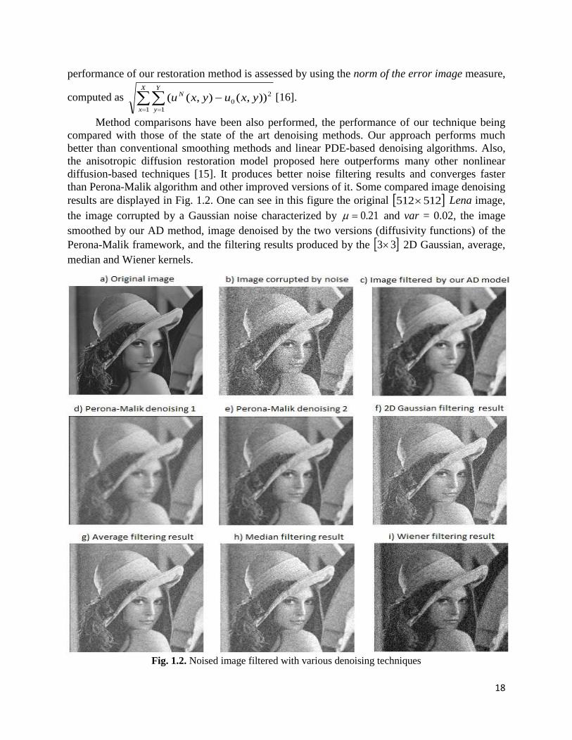
results are displayed in Fig. 1.2. One can see in this figure the original 512512 Lena image,
the image corrupted by a Gaussian noise characterized by 21.0 and var = 0.02, the image
smoothed by our AD method, image denoised by the two versions (diffusivity functions) of the
Perona-Malik framework, and the filtering results produced by the 33 2D Gaussian, average,
median and Wiener kernels.
Fig. 1.2. Noised image filtered with various denoising techniques
19
Table 1.1. Norm-of-the-error image values for several denoising algorithms
Our AD P-M 1 P-M 2 Gaussian Average Median Wiener 3101.5 3101.6 3109.5 3103.7 3104.6 3106 3108.5
Obviously, the best denoising result was produced by our model (c). The corresponding
norm of the error image values are registered in Table 1.1. The minimum NE value, representing
the best smoothing, corresponds to the AD approach described here. Our nonlinear PDE-based
restoration approach not only removes a high amount of image noise, but also preserves the
boundaries very well. Its edge-preserving character is also obvious from the above figure.
We have also investigated other edge-stopping functions, besides (1.13) and (1.17), and
achieved effective anisotropic diffusion schemes. A newly developed PDE restoration model is
0
0)(
,,0 uyxu
uuuudivt
uuK
(1.19)
where )()( uordruuK , ord () = order in evolving sequence, 2,3 , 0,1r and
8,1,
0for ,1
0 ,
)(log)(
)()(
10
2
)(
s
s
uKsuK
uKssuK , (1.20)
its image denoising results being disseminated in a paper under consideration (not yet published).
1.2.3. Image denoising approach based on diffusion porous media flow
We also designed a nonlinear filter for image noise removal based on the diffusion flow
generated by the porous media equation [18]. The proposed nonlinear diffusion-based restoration
model provides a robust edge-preserving smoothing, while also removing the staircasing effect.
It has the following form:
),0(,0)),((
),0(in ,0)),((),(
xtu
xtuxtt
u
(1.21)
where 0,0 uxu , represents a bounded domain of 2R with a sufficiently smooth
boundary and RR : is monotonically increasing,r
(0) 0 and lim ( ) .r
We demonstrate in [18] that PDE model (1.21) has a unique strong solution
1:[0, ) ( )u H that is given by the exponential formula uAn
tItu
n
lim)( , where the
nonlinear operator 1 1: ( )A D A H H is defined by the following equation:
( ), ( )Au u u D A (1.22)
20
with 1 1
0( ) ; ( )D A u L u H . In particular, (1.22) amounts to saying that the
implicit finite difference scheme 1 1 0, , 0,1,...,k k ku hAu u u g k where tk
h
, is
convergent to ( ).u t A rigorous mathematical investigation of the existence, uniqueness and
strength of this PDE model’s solution is provided in our 2013 article (see [18]).
One then determines the explicit version of the implicit scheme. The next iterative finite-
difference based explicit numerical approximation model is obtained:
i,jjiuu
uuuuuuu
ji
k
ji
k
ji
k
ji
k
ji
k
ji
k
ji
k
ji
),,(
4
0
0
,
11
,
11
1,
11
1,
11
,1
11
,1,
1
,
(1.23)
where k = 1,…,K. The initial degraded image is successfully filtered in K steps by using the
iterative scheme (1.23) with some properly selected parameters, and . The resulted Ku
represents the final image denoising result.
A proper selection of the parameter values is quite important and cannot be a priori
defined. The selection of K in our simulation was dictated by the many experiments performed in
specific examples. It turns out the selection of a high number of iterations, for example K > 40
value, could produce a blurring effect on the processed image, while using a low K value, such as
K < 5, may provide an unsatisfactory image smoothing result. Also, a great K value increases the
computational complexity of this image filtering process, producing a much higher computation
time. Also, using a large enough value, such as 5 , could increase the image degradation.
A very small parameter, like 1.0 , produces no visible restoration results. The parameter
must satisfy the condition )1,0(1
, for an efficient noise removal.
Our diffusion porous media flow based denoising algorithm was compared with other
well-known nonlinear diffusion schemes. In [18] we performed mathematically supported
method comparisons with the Perona-Malik framework, the PDE denoising model developed by
Kacur and Mikula [19], and the total variation model [11]. In order to perform these comparisons
we transformed our nonlinear diffusion model into an equivalent variational model, given by this
minimization problem:
2
)(0 1
2)((minarg
Huudxxuu
(1.24)
where )()( 11 HLu and is the potential function corresponding to the nonlinear
diffusivity function RR : .
Thus, the function 2
)(0 1 H
uuu represents a penalty term that forces the restored
image ( )u u x to stay close to the initial image. The fact that the distance from u to 0u is
taken in the norm 1 ( )|| ||
H that is considerably weaker than the
2 ( )L - norm used by the
Perona-Malik scheme, as well as the most diffusion techniques, has the advantage that it allows
to work with very degraded initial images that practically are not represented by Lebesgue

21
integrable functions but by distributions. However, it should be said that our model has a
considerable better denoising effect than Perona & Malik algorithm. Also, it outperforms the
Kacur-Mikula image restoration scheme that is based on a boundary value problem which
converges to a weak solution (see [19]). The present PDE technique is also more convenient that
the total variation model [11], that is constructed in a non-energetic space (the space of functions
with bounded variation) and so difficult to treat from the computational point of view. As a
matter of fact, by regularization necessary to construct a viable numerical scheme, the TV model
loses most of the theoretical advantages regarding the sharp edge detection and elimination of the
staircasing effect [20]. The staircasing effect, representing creation in the image of flat regions
separated by artifact boundaries [20], is common in denoising procedures with high smoothing
effect. Unlike other nonlinear diffusion based techniques, like Perona-Malik and its versions, this
restoration approach succeeds in removing this staircase effect, this fact representing another
important advantage of our PDE model.
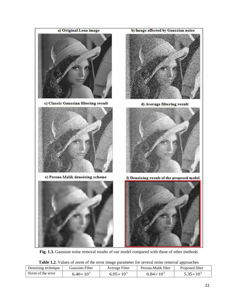
The diffusion porous media flow based denoising method described here was tested on
various image datasets, satisfactory filtering results being obtained. Hundreds of grayscale
images affected by various levels of Gaussian noise were filtered by using the presented
approach. The optimal noise reduction results were achieved using the following set of
parameters of the diffusion model: 2 , corresponding to the physical model of diffusion in
plasma, 5.1 and N = 20. One can see the image smoothing example based on these parameter
values that is displayed in Fig. 1.3. As we have already mentioned, numerous method
comparisons were also performed, the denoising results of our technique being compared against
the results obtained by other nonlinear diffusion based methods. Obviously, the proposed PDE
model outperforms not only both versions of the Perona-Malik method, but also some well-
known conventional filters, such as 2D Gaussian filter and the averaging filter.
So, the standard ]512512[ image of Lena is displayed in the grayscale form in Fig. 1.3
(a). Its version corrupted by an amount of Gaussian noise characterized by parameters 0.2 (mean)
and 0.02 (variance), is depicted in Fig. 1.3 (b). In Fig. 1.3 (c) there is displayed the image
smoothing result produced by the classic 33 Gaussian 2D filter kernel, while the noise
reduction obtained by the 33 averaging filter kernel is represented in Fig. 1.3 (d). The noise
removal achieved by the Perona-Malik scheme is displayed in Fig. 1.3 (e), while the denoising
result provided by our nonlinear PDE model is represented in Fig. 1.3 (f). One can observe in
these figures the better smoothing effect of our approach, its edge-preservation character and the
efficient removing of the staircasing effect.
The norm of the error image is also computed here, in order to assess the performance
levels of each denoising approach. These NE values corresponding to all these image filtering
techniques are registered in the next table. As one can see in Table 1.2, the porous media
equation based smoothing technique developed by us outperforms all the other image filters,
minimizing the respective error (see the lowest value, 31015.5 ). Also, our denoising algoritm
executes quite fast, given its low time complexity. The values of the Peak Signal-to-Noise Ratio
(PSNR) measure [2,3] were also computed to asses the method performance and gave us the
same conclusion.
22
Fig. 1.3. Gaussian noise removal results of our model compared with those of other methods
Table 1.2. Values of norm of the error image parameter for several noise removal approaches
Denoising technique Gaussian Filter Average Filter Perona-Malik filter Proposed filter
Norm of the error 31040.6 31005.6
31084.6 31035.5

23
1.2.4. Fourth order diffusion models for image noise reduction
The fourth order PDE models are more effective at staircasing effect removing during the
image smoothing process than the second-order PDEs. The most popular fourth-order PDE
restoration scheme is the nonlinear isotropic diffusion method proposed by Y. L. You and M.
Kaveh in 2000.
Also, the static and video images, especially those based on ultrasounds, are often
affected by speckle noise, which represents a multiplicative noise that is locally correlated and
prevents a proper feature extraction and analysis from the affected images. In recent years
numerous speckle denoising techniques have been developed. The most important are the Frost
filtering [21], that replaces the pixel of interest with the weighted sum of the values in a moving
kernel, the Discrete Wavelet Transform based approaches, using complex DWT - 2D and DWT -
3D [22], and the fourth-order PDE based smoothing techniques derived from You-Kaveh [23].
We developed an effective nonlinear diffusion-based method for removing both the
Gaussian and speckle noise from images and video sequences. This image denoising approach
proposed in [24] is based on the following fourth-order PDE model:
0
uu
t
u (1.25)
where the Laplacian uu 2 and represents a diffusivity function modelled as following:
ks
ss
2 (1.26)
where k > 0 represents a chosen constant. Obviously, this function is monotone decreasing and
converges to 0. Thus, it satisfies the main conditions of a noise filtering function [23]:
00
0lim
ss (1.27)
In our 2011 paper one demonstrates rigorously the well-posedness of the problem (1.25)
[24]. Thus, we prove that this problem is indeed well posed if the function )(uguuu
is continuous and monotonically nondecreasing (see [24] for more).
Then we perform a robust discretization of the proposed PDE-based model [24]. We set
uud jkjkjk ,,, , where ujk , is a finite-difference based discretization of u , and obtain
the following iterative approximation scheme for the differential model:
i
jk
i
jk
i
jk
i
jk
i
jk
i
jk
i
jk ddddduu ,1,1,,1,1,
1
, 4
, (1.28)
where .,...,2,1 ni We also impose some boundary value conditions of zero flux boundary type,
which have the following form for an NM image:
Nkuuuu
Mjuuuu
MkMkkk
jjjNjN
,...,0,,
,...,0,,
,1,0,1,
,0,1,,1 (1.29)
24
A lot of noise removal experiments using the proposed PDE based technique have been
conducted, satisfactory results being achieved. The iterative scheme (1.28) has been successfully
applied on hundreds sonar images and video frames affected by noise. That image noise has been
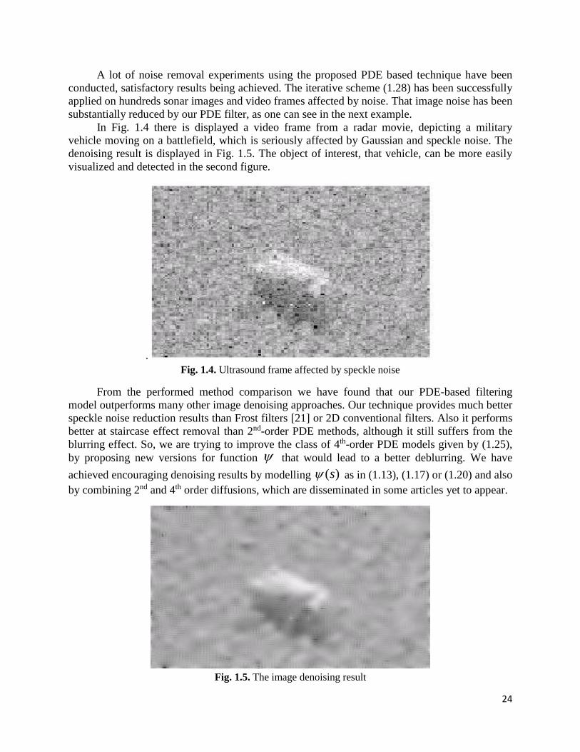
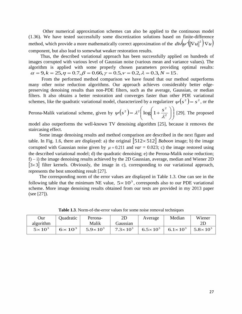
substantially reduced by our PDE filter, as one can see in the next example.
In Fig. 1.4 there is displayed a video frame from a radar movie, depicting a military
vehicle moving on a battlefield, which is seriously affected by Gaussian and speckle noise. The
denoising result is displayed in Fig. 1.5. The object of interest, that vehicle, can be more easily
visualized and detected in the second figure.
.
Fig. 1.4. Ultrasound frame affected by speckle noise
From the performed method comparison we have found that our PDE-based filtering
model outperforms many other image denoising approaches. Our technique provides much better
speckle noise reduction results than Frost filters [21] or 2D conventional filters. Also it performs
better at staircase effect removal than 2nd-order PDE methods, although it still suffers from the
blurring effect. So, we are trying to improve the class of 4th-order PDE models given by (1.25),
by proposing new versions for function that would lead to a better deblurring. We have
achieved encouraging denoising results by modelling )(s as in (1.13), (1.17) or (1.20) and also
by combining 2nd and 4th order diffusions, which are disseminated in some articles yet to appear.
Fig. 1.5. The image denoising result
25
1.3. Variational PDE techniques for image denoising and restoration
The variational approaches have important advantages in both theory and computation,
compared with other techniques. They can achieve high speed, accuracy and stability using the
extensive results of the numerical PDE algorithms. Variational PDE methods represent useful
tools for solving various image processing and analysis tasks, one of them being the image
denoising.
Each variational denoising technique is based on a minimization of an energy functional
composed of a data component and a smoothing term. The variational denoising and restoration
approaches differ with regard to the modeling of these components.
An influential variational image smoothing model was developed by Rudin, Osher and
Fetami in 1992 [25]. Their filtering technique, named Total Variation (TV) denoising, is based
on the minimization of the TV norm. TV denoising is remarkably effective at simultaneously
preserving image edges whilst smoothing away noise in flat regions, but it also suffers from the
staircasing effect and its corresponding Euler-Lagrange equation is highly nonlinear and difficult
to compute [25]. In the last two decades, numerous PDE techniques which improve this classical
variational scheme have been proposed [26]. We developed two variational models that provide
an efficient noise reduction while eliminating the staircasing effect [27,28]. The proposed
techniques are described in the next subsections.
1.3.1. A robust variational PDE model for image denoising
The general variational framework used for image denoising and restoration is based on
the following the energy functional:
0 ,)(22
0
uuuuE (1.30)
where the function
is the regularizer, or penalizer, of the smoothing term and represents
the regularization parameter or smoothness weight [29].
We modeled a robust smoothing component, based on a novel penalizer function and a
proper value of the smoothness weight [27]. Thus, we consider in [27] the following regularizer,
,0,0: :
)1,0(,,,,0 ;ln 2
ksss
ks (1.31)
We use some proper values for the penalizer’s parameters. Then, we compute a minimizer
for the energy functional given by (1.30), using the function provided by (1.31):
dxdyuuuuEuUuUu
22
0min )(minarg)(minarg (1.32)
The minimization result minu represents the restored image. The minimization process is
performed by solving the next Euler-Lagrange equation [26,29,30]:
26
0'0'202
0
uudivuu
uudivuu
(1.33)
This leads to the following PDE equation:
02'
uuuudiv
t
u
(1.34)
where the positive function ' is obtained by computing the derivative of the function given by
(1.31):
2
2
2's
kss (1.35)
So, the partial differential equation (1.34) becomes
0
0
2
2
),,0( uyxu
uuu
u
kudiv
t
u
(1.36)
One can demonstrate the PDE model given by (1.36) converges to a unique strong
solution, that is min* uu . In [27] we propose a robust discretization scheme for solving it. The
numerical approximation of our PDE model uses a 4-NN discretization of the Laplacian operator
[27]. So, from (1.34) we obtain:
02'),,()1,,(
uuuudivtyxutyxu
(1.37)
that leads to
0
)(
,
2
,
1 )()('uu
tutuuupNq
qpqp
tt
(1.38)
where 1 ,0 , t =1, …,N, )1,(),1,(),,1(),,1()( yxyxyxyxpN , p = (x, y) and
),(),()(, tputqutu qp .
The variational PDE model developed by us converges fast to the solution minuu N , the
parameter N taking quite low values. The effectiveness of the proposed denoising technique and
its numerical approximation is proved by the satisfactory image smoothing results obtained from
our experiments [27].
27
Other numerical approximation schemes can also be applied to the continuous model
(1.36). We have tested successfully some discretization solutions based on finite-difference
method, which provide a more mathematically correct approximation of the uudiv 2
'
component, but also lead to somewhat weaker restoration results.
Thus, the described variational approach has been successfully applied on hundreds of
images corrupted with various level of Gaussian noise (various mean and variance values). The
algorithm is applied with some properly chosen parameters providing optimal results:
15,3.0,2.0,5.0,66.0,7.0,25,9 Nk .
From the performed method comparison we have found that our method outperforms
many other noise reduction algorithms. Our approach achieves considerably better edge-
preserving denoising results than non-PDE filters, such as the average, Gaussian, or median
filters. It also obtains a better restoration and converges faster than other PDE variational
schemes, like the quadratic variational model, characterized by a regularizer 22 ss , or the
Perona-Malik variational scheme, given by
2
222 1log
ss
[29]. The proposed
model also outperforms the well-known TV denoising algorithm [25], because it removes the
staircasing effect.
Some image denoising results and method comparison are described in the next figure and
table. In Fig. 1.6, there are displayed: a) the original 512512 Baboon image; b) the image
corrupted with Gaussian noise given by 211.0 and var = 0.023; c) the image restored using
the described variational model; d) the quadratic denoising; e) the Perona-Malik noise reduction;
f) – i) the image denoising results achieved by the 2D Gaussian, average, median and Wiener 2D
33 filter kernels. Obviously, the image in c), corresponding to our variational approach,
represents the best smoothing result [27].
The corresponding norm of the error values are displayed in Table 1.3. One can see in the
following table that the minimum NE value, 3105 , corresponds also to our PDE variational
scheme. More image denoising results obtained from our tests are provided in my 2013 paper
(see [27]).
Table 1.3. Norm-of-the-error values for some noise removal techniques
Our
algorithm
Quadratic Perona-
Malik
2D
Gaussian
Average Median Wiener
2D 3105 3106 3109.5 3103.7 3105.6 3101.6 3108.5
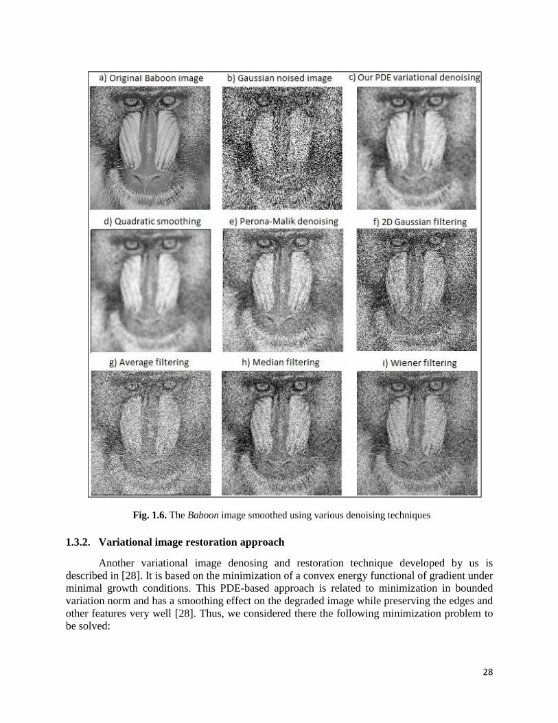
28
Fig. 1.6. The Baboon image smoothed using various denoising techniques
1.3.2. Variational image restoration approach
Another variational image denosing and restoration technique developed by us is
described in [28]. It is based on the minimization of a convex energy functional of gradient under
minimal growth conditions. This PDE-based approach is related to minimization in bounded
variation norm and has a smoothing effect on the degraded image while preserving the edges and
other features very well [28]. Thus, we considered there the following minimization problem to
be solved:
29
dxxuxuxuuXu
22
0)(
min )())()((2
1minarg (1.39)
where 0u is the initial image, affected by noise. In order for the minimization problem to be well
posed one assumes that is convex and lower semicontinous and X(Ω) must be taken, in
general, as a distribution space on Ω. The following regularizer function is considered for this
PDE variational model: .,,1log1log 212211 ssssssss The minimization
problem is then associated with a boundary value problem having the following form:
on ,0),(
in ,0
vu
udivu x
(1.40)
where represents the subdifferential of . In [28] we demonstrate that the PDE variational
problem (1.39) has a unique minimizer that represents the weak solution to the boundary value
problem (1.40).
A numerical approximation based on the discretization of the variational PDE model is
then provided (see [28] for more). Thus, we obtain the following explicit finite difference
scheme:
0
1,1,,1,,1
1
, 221 ij
n
ji
n
ij
n
ji
n
ij
n
ji
n
ij
n
ji
n
ij
n
ij
n
ji
n
ij
n
ji kuukdukdukbukdkbkukbu
(1.41)
where
)(),( ,11,,,1,1,
n
ji
n
ji
n
ji
n
ji
n
ji
n
ji uuBduuBb (1.42)
with
2)1(
2)(
u
uuB (1.43)
This explicit approximation scheme is stable and convergent for 5.0k [28]. The
iterative algorithm that applies the scheme on the evolving image for n = 1, 2, … , N, produces
an efficient smoothing Nu of the initial noisy image 0
0 uu in a relatively low number of
iterations, N.
The proposed variational approach has been tested on numerous images affected by
Gaussian noise, these experiments proving its restoration effectiveness. Method comparisons
have been also performed and we have found that our technique outperforms the most
conventional denoising filters, such as Gaussian, Laplacian, Laplacian of Gaussian (LoG),
Wiener adaptive filter, average, and median filter. Some color image denoising results are
displayed in Fig. 1.7. One can see that our PDE approach provides a better noise reduction than
average, median and Wiener filters and also corresponds to the minimum error (NE) value.

30
Fig. 1.7. Method comparison: restoration results obtained by various image filters

31
1.4. Mathematical models for media feature vector classifiers and metrics
If in the previous sections we described several mathematical models related to image
processing, herein we present some machine learning models related to image, and generally
media, analysis. As one will see in future chapters, digital media analysis consists of the
extraction of meaningful information from media objects, such as images, videos and sounds,
and produces feature vectors that describe the content of these objects.
The feature vectors are very useful in some important media analysis processes like
recognition, segmentation or tracking. These analysis procedures work with distance values,
therefore they require proper metrics to measure the distances between these feature vectors. The
conventional metrics, such as the well-known Euclidian distance, cannot always be used,
because the media feature vectors can be computed in various forms, depending on the featured
object and the intended analysis goal. These feature vectors could often represent complex
structures and not common vectors or matrices. Even if they represent common vectors (1D, 2D,
3D), their dimensions may differ, therefore the distance between them cannot be computed using
conventional metrics.
For this reason, we have introduced some special metrics for certain media feature vectors.
Their mathematical models are described in the next two subsections. The proposed metrics were
used by various classifiers modeled by us. Any media pattern recognition process consists of a
feature extraction operation and a classification of the resulted media feature vectors. We
developed both supervised and unsupervised media feature vector classifiers during our research
activity. Some supervised recognition (classification) techniques will be presented in the next
chapters. Several automatic unsupervised classification models are described in the last two
subsections.
1.4.1. A Hausdorff-derived metric for different-sized 2D feature vectors
Some important media analysis tasks approached by us require computing distances
between different-sized two-dimension feature vectors that have one equal dimension. As we
will see in the next chapter, the vocal recognition techniques described there use 2D speech
feature vectors of this type (see selected paper 2 in [31]). We also developed a reputation
system based on an automatic web community user recognition approach that models feature sets
containing vectors having only one equal dimension [32].
To measure distances between such feature vectors, we proposed in [31] a special metric
working properly for matrices having at least one equal size, that was further investigated in next
papers [32,33]. It is derived from the Hausdorff-Pompeiu metric for sets [34]. If X and Y are two
compact subsets of a metric space M, the Hausdorff-Pompeiu distance between them, dH (X,Y), is
defined as the minimal number r such that the closed r-neighborhood of any x in X contains at
least one point y of Y and vice versa. So, if dist(x, y) denotes the distance in M, then the
Hausdorff-Pompeiu metric is computed as follows:
)},(infsup),,(infsupmax{),( yxdistyxdistYXdXxYyYyXx
H
(1.44)
We have derived this metric, considering 2D feature vectors instead of sets [31-33]. Thus,
we represent the two feature vectors to be compared as two matrices having the same number of
32
rows: mnijaA )( and pnijbB )( . Two more helping vectors are introduced: 1)( piyy
and 1)( mizz , then,
pi
ipyy
0
max and mi
imzz
0
max are computed. With these notations we
created a new metric d having the following form:
AzByAzByBAdp
mm
pyzzy 1111
infsup,infsupmax),( (1.45)
This restriction based metric represents the Hausdorff-Pompeiu distance between the sets
)1:( p
yyB and )1:( m
zzA in the metric space Rn, so, it can be written as:
))1:(),1:((),( mpH zzAyyBdBAd (1.46)
From
m
j
jij
p
k
kik zaybAzBy11
, one gets
m
j
jij
p
k
kiknin
zaybAzBy11
1max ,
which leads to:
m
j
jij
p
k
kiknizy
nzy
zaybAzBym
pm
p 1111111
maxinfsupinfsup (1.47)
This can be seen as a max min optimization problem and according to the classical J. von
Neumann min max theorem [35] we have:
nyznzy
AzByAzByp
mmp
1111
supinfinfsup (1.48)
Moreover, the saddle point ),( 00 zy of this problem could be computed by solving the next
system:
),(, ,
0
021
2
1zyN
AzBy
AzBy
ny
nz
(1.49)
where ),( zyN is the normal cone to the set 1 ;1 ; mp
zzyy and which can be
expressed in terms of the Lagrange multipliers. Finally, zy , represent gradients taken in
generalized sense of convex analysis (see [36]). However, since (1.48) is hard to compute for
large dimensions of A and B we replace it by a simpler one. So, the set 1| p
yy is replaced

33
with
components
}1,...,0,0{},...,0,...,1,0{},0,...,0,1{
p
F and the set 1| m
zz with
components
}1,...,0,0{},...,0,...,1,0{},0,...,0,1{
m
G [36]. Thus, we may take:
ijiknimjpk
nGzFy
abAzBy 111
supinfsupinfsup (1.50)
While the above formula is not identical with (1.48), it can be regarded as a good
approximation for it. As a matter of fact, we replaced optimization problem on convex set
1 ;1 ; mp
zzyy with one on a simpler GF on its boundary. Similarly, we
could replace AzByp
myz
11
infsup in (1.44) with ijik
nipkmi
ab 111
supinfsup . Thus, the transformed
formula (1.45) becomes the following Hausdorff-based distance:
ijiknipkmi
ijiknimipk
ababBAd111111
supinfsup,supinfsupmax),( (1.51)
The resulted nonlinear function d verifies the three main properties of a metric: positivity
( 0),( BAd ), symmetry ( ),(),( ABdBAd ) and triangle inequality ( ),(),( CBdBAd
),( CAd ). So, this Hausdorff derived function represents a distance, although it does not
represent the standard Hausdorff-Pompeiu metric anymore [36]. It defines a new metric topology
on the space of all matrices {A}, that is not equivalent but comparable with that induced by the
Hausdorff topology [36]. This metric has been successfully used in the classification processes,
representing a powerful discriminator between feature vectors.
1.4.2. A special metric for complex feature vectors
The feature vectors corresponding to some media objects do not represent always 1D, 2D
or 3D vectors. Often they represent very complex structures, therefore the distances between
them cannot be computed using conventional metrics, like the Euclidian distance. For example,
some biometrics-related image analysis techniques, such as face [37] and fingerprint recognition
[38], could produce this kind of feature vectors. These methods developed by us identify a set of
keypoints in the image, such as SIFT points (for faces) [37] and minutiae points (for fingerprints)
[38], and model a feature vector for each keypoint. Such a feature vector could be a complex
structure, whose components may represent names, locations, orientations or codify other
information. The global feature vector is composed of all the feature vectors corresponding to the
keypoints (see selected paper 4 [38]).
We have modeled a generic metric for this type of feature vectors that is based on the
number of matches between them. Therefore, if ],....,[ 1 nvvv and ],....,[ 1 mwww represent
two different-sized feature vectors of this kind, then the distance between them is computed as
following:

34
)),((2
),( wvMcardnm
wvd
(1.52)
where card (M (v, w)) is the number of pairings (matches) between v and w. Thus, ),( ji wv
represents a match between these feature vectors if iv jw , which means these components
are closed enough to each other, in terms of the criteria related to that image analysis task [37-
39]. The set of the matches is modeled as:
jtikwvMtkwvjiwvM ji &),(,&|,),( (1.53)
where
Twvdistwv jiji ),( (1.54)
where dist is a proper metric that works for the feature vectors iv and jw , and T is a properly
selected low threshold value.
The function d satisfies the main properties of a metric [37-39]. The non-negativity is
demonstrated easily as follows:
0),(2
),min()),((
wvdnm
nmwvMcard
(1.55)
The Leibniz rule is satisfied because:
wvnmwvMcardnm
wvMcardwvd
)),((2
)),((0),(
(1.56)
Obviously, the symmetry property is satisfied by d:
),(),(),(),( vwdwvdvwMwvM
(1.57)
The sub-additivity, or triangle inequality, is also verified because we have:
)),(()),(()),((),(),(),( uvMcarduwMcardwvMcardnuvduwdwvd
(1.58)
We introduced M (u, v, w), the set of matches between all the three feature vectors, and
),( wvM u , representing the set of matches between v and w but cannot be found in u. Obviously,
)),(()),,(()),(( wvMcardwvuMcardwvMcard u , so (1.58) is equivalent to:
)),(()),(()),(()),,(( uvMcardwuMcardwvMcardwvuMcardn wvu (1.59)
which is true because )),(()),(()),,(( wuMcardwvMcardwvuMcardn vu .

35
1.4.3. Automatic unsupervised classification algorithm
The machine learning techniques represent essential tools for our research. While
biometric systems, described in the next chapter, are mostly based on supervised classification
(recognition) algorithms, the image analysis methods, described in the third chapter, make use of
unsupervised classification models. An unsupervised classification, or clustering, approach must
be able to group a set of feature vectors (and consequently the corresponding media objects) in a
number of classes (clusters), having no previous knowledge about these classes. In fact the only
available knowledge about them could be their number.
If the number of classes is a priori known, or set interactively by the user, then we have a
semi-automatic unsupervised classification technique. Semi-automatic clustering methods, such
as hierarchical agglomerative clustering and K-means algorithms, have been widely used by us.
Very often, the number of classes cannot be known, therefore some automatic clustering
solutions are required. We have proposed several automatic classification techniques that are
described in this subsection and the next one [39-42]. The clustering model described here
represents an extended and automatic version of the hierarchical agglomerative clustering, or
region growing, scheme [39]. If },...,{ 1 nVV represents a sequence of media feature vectors to
be classified, the automatic unsupervised classification algorithm developed by us to solve this
task is modeled as following:
1. A distance set is initialized: D
2. One starts the classification process with all the feature vectors as the n initial clusters:
}{},...,{ 11 nn VCVC .
3. Each feature vector is labeled: iVCni i )( ],,1[ .
4. At each iteration one computes the overall minimum distance between clusters and merges
those being at that distance from each other:
jjiijiCl CCCCdCCdji ,),( , min , (1.60)
where
jiClnji
CCdd ,min],1[
min
(1.61)
and the distance between the clusters could be computed as a single linkage clustering metric
wvdCCdji CwCv
jiCl ,min,,
, (1.62)
a complete linkage clustering metric
),(max),(,
wvdCCdji CwCv
jiCl
, (1.63)
or an average linkage clustering, described as

36
)()(
),(
),(ji
Cv Cw
jiClCcardCcard
wvd
CCdi j
, (1.64)
where d is a proper metric for the feature vectors v and w [39].
5. Minimum distance is then registered: }{ mindDD .
6. When a single cluster is obtained, a new clustering process is performed on the distance set
D, using a hierarchical agglomerative clustering (region-growing) algorithm: steps 2 and 3
are applied, then step 4 is repeated until the number of clusters becomes K = 2. Two classes
containing distance values are thus obtained.
7. One element from each class is randomly selected and the two distance values are then
compared. The class corresponding to the greater value represents the set of large distances,
let it be lD . The smaller value belongs to the set of small distances, sD . Obviously,
sl DDD .
8. For any small distance, it searches for all pairs of vectors corresponding to it and the feature
vectors from each identified pair are inserted in the same class:
iVCdistVVdifnjiDdist jjis )( ) ,( ],,1[, (1.65)
The resulted labeling, )}(),...,({ 1 nVCVC , represents the final media feature vector
classification result [39]. The described automatic clustering algorithm has been successfully
applied in various recognition tasks, and also in important domains like database indexing.
1.4.4. Automatic clustering models based on validity indexes
We also developed some robust automatic unsupervised classification models that use
semiautomatic clustering approaches and validation index based measures [40-42]. Thus, we
considered the same feature set, },...,{ 1 nVV , to be clustered. An integer value nT ,1
representing the maximum number of possible feature vector clusters was selected first. A high T
value could lead to better classification results, but also raises the computation volume and the
time complexity of the classification process. Usually, we have used the value
2
nT in our
experiments.
For each TK ,1 one applied a semi-automatic unsupervised classification procedure to
the feature vector set [40-42]. We generally used a K-means algorithm [40,42] or a hierarchical
agglomerative procedure [41] for this clustering task, but some other unsupervised recognition
solutions, like Fuzzy K-Means [43] or Self Organizing Maps (SOM) [44], could also be used.
In the previous sub-section we described how a hierarchical agglomerative clustering
algorithm works: each observation starts in its own cluster, and pairs of clusters are merged as
one moves up the hierarchy. The K-means clustering, proposed by MacQueen in 1967, represents
one of the simplest unsupervised learning algorithms [45]. In statistics and machine learning, K-
means is a method of cluster analysis which aims to partition n observations into K clusters in
which each observation belongs to the cluster with the nearest mean. The clustering procedure is
composed of the following steps:

37
1. One selects K initial centroids, as much as possible far away from each other, each centroid
representing a point in the feature vector space.
2. Each feature vector is associated to the closest centroid (in terms of the used distance)
3. The centroids of the obtained clusters are recomputed, as means of the vectors in those
clusters.
4. Steps 2 and 3 are repeated until the centroids of the classes no longer change their positions.
In the next phase, one determines the optimal number of clusters, from 1 to T. Some
cluster validity indexes are used for this purpose [40-42]. We modeled a measure based on a
combination of Dunn and Davies-Bouldin validation indexes in [40]. The Dunn index aims to
maximize the inter-cluster distances and minimize the intra-cluster distances [46]. The number of
clusters that maximizes the Dunn index is considered the optimal number of clusters. This
validity index has a linear time complexity, its computational complexity being O (n), this fact
representing an advantage. Its main disadvantage is the vulnerability for noise in the data. The
index proposed by Davies and Bouldin is a function of the ratio of the sum of within-cluster
scatter to between-cluster separation [47]. Its lowest value indicates an optimal clustering
operation. The Davies-Bouldin index becomes computationally expensive when the number of
clusters grows very large.
Therefore, for each K we obtain the feature vector clusters KClCl ,...,1
. Then, the optimal
number of classes is determined by performing the following minimization [40]:
)(
1)(minarg
],1[ KDKDBK
TKoptim (1.66)
where the Davies-Bouldin index is computed as
ji
jiK
iji CCd
CldCld
KKDB
,max
1)(
1
(1.67)
and the Dunn index is obtained as
k
Kk
ji
ijKi Cld
CCdKD
],1[
],1[ max
,minmin)( (1.68)
where iC is the centroid of the cluster iCl , while iCld represents the intra-cluster distance
of iCl , that is the absolute squared distance between all pairs of points in that cluster. So, the
final feature vector classification result is optimKClCl ,...,1 .
The automatic clustering models described here have been successfully used by numerous
media pattern recognition and indexing techniques developed by us. The voice recognition [41],
image classification [48], shape recognition [40], image segmentation [42] and media indexing
[33] approaches using these clustering solutions are described in the next two chapters.

38
1.5. Conclusions
In this chapter we described some robust mathematical models that have been developed
by us to facilitate the biometric and computer vision techniques presented in the following
chapters. These models are grouped into two main categories. The first one contains the PDE-
based mathematical models for image and video enhancement, while the second category
contains machine learning models.
We proposed in our recently published papers some effective PDE-based image denoising
and restoration techniques that provide very good results and outperform not only the
conventional filtering methods but also many other PDE-based approaches. Our PDE denoising
algorithms are divided into diffusion-based methods and variational approaches. We brought
important original contributions in the diffusion-based restoration field, which were described in
this chapter. Thus, a linear diffusion technique, based on a 2nd order hyperbolic PDE model, was
presented first. It reduces substantially the Gaussian noise and also enhances the image contrast.
Nonlinear diffusion-based smoothing algorithms were also described in this chapter. Thus,
we provided a detailed overview of the state of the art nonlinear diffusion techniques derived
from the Perona-Malik framework. A novel anisotropic diffusion-based model developed by us
is also introduced and compared with those state of the art approaches. Another proposed PDE-
image filtering solution, which could be also represented as a variational problem, is based on a
diffusion porous media flow and outperforms some influential PDE denoising schemes, like
Perona-Malik, TV and Kacur-Mikula models. A 4th-order PDE diffusion model that achieves
satisfactory Gaussian and speckle noise reduction results was also described here. Two PDE
variational models developed by us are described in this chapter. They provide an efficient noise
reduction, obtaining much better results than conventional filters. Also, our techniques overcome
the drawbacks of other existing variational models, such as the TV model.
All the PDE-based image filtering solutions described in this chapter represent original and
effective denoising techniques developed by us and published in some prestigious international
journals [5,15,16,18,24,27,28]. A rigorous mathematical treatment was performed for each
proposed PDE model, its convergence and stability being mainly investigated. More detailed
mathematical investigations of these models are provided in those papers disseminating our
research results in PDE-based image enhancement domain. Robust discretization schemes were
constructed for all these differential models and explained in this chapter.
The effectiveness of these numerical approximation algorithms was demonstrated by the
successful denoising experiments, some of them described in the chapter. All PDE denoising
models proposed by us have also a strong edge-preserving character. Method comparisons were
also provided for all our restoration techniques. We have found that our PDE filtering schemes
not only achieve much better results than conventional algorithms, but also outperform the
influential schemes of the same class. Thus, our nonlinear diffusion methods outperform the
Perona-Malik models, while our variational approaches outperform the TV denoising. Since all
our described PDE techniques succeed also in removing the staircasing effect, they can represent
better denoising solutions than many state of the art PDE-based technologies. Also these
methods can be applied successfully to the edge detection domain, and consequently to object
detection.
Our original contributions to media feature vector classification domain, disseminated in
important scientific publications [31-33,37-39], were then described. The two novel metrics
introduced by us represent important contributions in this field, because they can perform some
39
difficult tasks that conventional metrics are unable to solve: measuring the distances between
different-sized feature vectors or special feature vectors representing not matrices but complex
structures. A robust mathematical treatment is provided by us for each metric. Also, these
proposed metrics can be applied successfully to feature vectors belonging to various media,
eventually adapted to those media. So, our metric derived from the Hausdorff-Pompeiu metric
for sets is used not only for the DDMFCC-based 2D speech feature vectors, but also for 2D
video feature vectors. Our second metric represents a similarity metric that is specially modeled
for images whose content is characterized by some key points. It is applied with some adaptations
to both SIFT-based facial feature vectors and minutiae-based fingerprint feature vectors.
The proposed automatic unsupervised classifiers, described in the last section, constitute
other significant machine learning contributions. Our media feature vector clustering models,
derived from semi-automatic clustering algorithms, like region-growing, or using these semi-
automatic clustering solutions in combination with some validation index based measures, are
very useful to any automatic unsupervised recognition task. For this reason, our classification
approaches are applied successfully to both biometrics and computer vision domains.
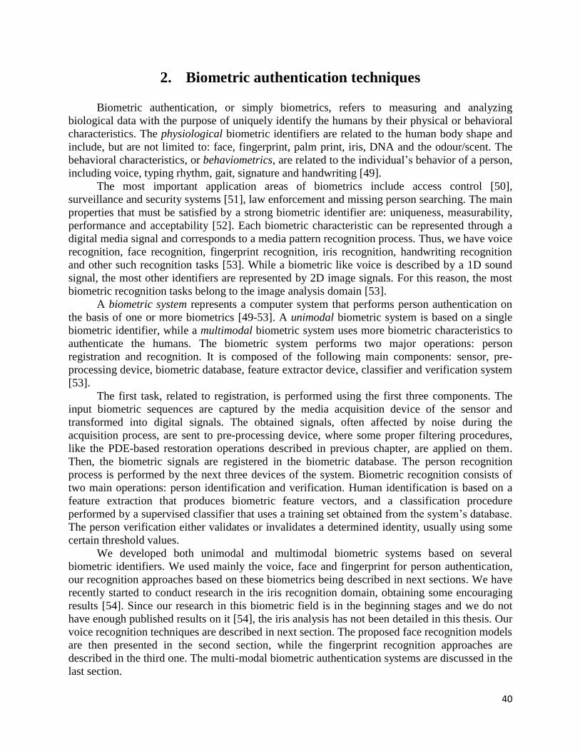
40
2. Biometric authentication techniques
Biometric authentication, or simply biometrics, refers to measuring and analyzing
biological data with the purpose of uniquely identify the humans by their physical or behavioral
characteristics. The physiological biometric identifiers are related to the human body shape and
include, but are not limited to: face, fingerprint, palm print, iris, DNA and the odour/scent. The
behavioral characteristics, or behaviometrics, are related to the individual’s behavior of a person,
including voice, typing rhythm, gait, signature and handwriting [49].
The most important application areas of biometrics include access control [50],
surveillance and security systems [51], law enforcement and missing person searching. The main
properties that must be satisfied by a strong biometric identifier are: uniqueness, measurability,
performance and acceptability [52]. Each biometric characteristic can be represented through a
digital media signal and corresponds to a media pattern recognition process. Thus, we have voice
recognition, face recognition, fingerprint recognition, iris recognition, handwriting recognition
and other such recognition tasks [53]. While a biometric like voice is described by a 1D sound
signal, the most other identifiers are represented by 2D image signals. For this reason, the most
biometric recognition tasks belong to the image analysis domain [53].
A biometric system represents a computer system that performs person authentication on
the basis of one or more biometrics [49-53]. A unimodal biometric system is based on a single
biometric identifier, while a multimodal biometric system uses more biometric characteristics to
authenticate the humans. The biometric system performs two major operations: person
registration and recognition. It is composed of the following main components: sensor, pre-
processing device, biometric database, feature extractor device, classifier and verification system
[53].
The first task, related to registration, is performed using the first three components. The
input biometric sequences are captured by the media acquisition device of the sensor and
transformed into digital signals. The obtained signals, often affected by noise during the
acquisition process, are sent to pre-processing device, where some proper filtering procedures,
like the PDE-based restoration operations described in previous chapter, are applied on them.
Then, the biometric signals are registered in the biometric database. The person recognition
process is performed by the next three devices of the system. Biometric recognition consists of
two main operations: person identification and verification. Human identification is based on a
feature extraction that produces biometric feature vectors, and a classification procedure
performed by a supervised classifier that uses a training set obtained from the system’s database.
The person verification either validates or invalidates a determined identity, usually using some
certain threshold values.
We developed both unimodal and multimodal biometric systems based on several
biometric identifiers. We used mainly the voice, face and fingerprint for person authentication,
our recognition approaches based on these biometrics being described in next sections. We have
recently started to conduct research in the iris recognition domain, obtaining some encouraging
results [54]. Since our research in this biometric field is in the beginning stages and we do not
have enough published results on it [54], the iris analysis has not been detailed in this thesis. Our
voice recognition techniques are described in next section. The proposed face recognition models
are then presented in the second section, while the fingerprint recognition approaches are
described in the third one. The multi-modal biometric authentication systems are discussed in the
last section.
41
2.1. Voice recognition approaches using mel-cepstral analysis Human voice represents a behavioural biometric identifier, although it could also be considered a physiological feature, because every person has a different pitch. Voice (speaker) recognition is the computational task of validating users’ claimed identity using characteristics extracted from their voices. A speaker recognition system is able to recognize who is speaking on the basis of individual information included in the speech signals [55]. Speaker recognition technology is successfully used in controlling the access to various services such as banking by telephone, database access services, information services, voice mail, security control for confidential information areas, and remote access to computers [55]. Audio surveillance systems also make use of voice recognition techniques. The voice recognition approaches can be divided into text-dependent (speech-dependent) and text-independent (speech-independent) techniques. The former methods discriminate the individuals based on the same spoken utterance and deal with cooperative subjects [31]. The latter techniques do not rely on a specific speech and deal with non-cooperative subjects [56], being useful for surveillance applications. As any biometric recognition system, the speaker recognition encompasses both person identification and verification. Human voice identification represents the process of determining which speaker provides a given vocal utterance, consisting of a feature extraction process and a classification one. Depending on the character of its classification stage, the speaker recognition can be either supervised or unsupervised. Speaker verification, on the other hand, represents the procedure of accepting or rejecting the identity claim of a previously identified speaker.
We developed both text-dependent [31] and text-independent voice recognition techniques
[57], and also both supervised [36] and unsupervised recognition approaches [41]. We have
achieved much better speaker recognition results in the speech-dependent case, so we describe
only the text-dependent approaches in this thesis. Since the Mel Frequency Cepstral Coefficients
(MFCCs) represent the dominant features used in speech and speaker recognition domains [58],
we proposed a voice feature extraction based on the mel-cepstral analysis for these methods. The
MFCC-based vocal feature extraction is described in the next subsection. In the second
subsection, a supervised speech-dependent voice recognition approach is proposed. Then, an
automatic unsupervised speaker recognition algorithm is described in the last subsection.
2.1.1. MFCC-based speech feature extraction solutions
There are various speech feature extraction solutions used by the voice recognition
systems. The most popular are the MFCC analysis, Linear Predictive Coding (LPC) analysis, and
the autoregressive (AR) coefficients. The speaker recognition techniques developed by us are
based on AR coefficients [59,60] or MFCC analysis [31,36,41,53] in the feature extraction stage.
We describe here a robust MFCC-based voice analysis on whose basis we modeled some
efficient speech feature vectors for speaker recognition. Thus, we consider a vocal sequence
represented by a 1D digital signal, to be featured, and perform a short-time analysis on it. The
speech signal is divided into overlapping frames with 256 samples and overlaps of 128 samples
[31,33,57]. Each resulted segment is then windowed, by multiplying it with a Hamming window
of 256 coefficients. The spectrum of each windowed sequence was then computed, by applying
the FFT (Fast Fourier Transform) to it (see selected paper 2, Barbu 2005 [31]).
The cepstrum of each windowed frame could be determined by applying the inverse
Fourier transform to its log-spectrum, but we considered the melodic cepstrum a much better
featuring solution. The regular frequencies were translated to a scale that is more appropriate for

42
human speech [33,36,53]. The mel-scale approximates the human auditory system's response
more closely than the linearly-spaced frequency bands used in the normal cepstrum. The
difference between the cepstrum and the mel-frequency cepstrum is that in the MFC, the
frequency bands are equally spaced on the mel scale. The mel-frequency cepstral coefficients
(MFCCs) were obtained as following:
1. The windowed signal was processed using FFT.
2. The powers of the spectrum obtained above were mapped onto the mel scale, using
triangular overlapping windows.
3. The logs of the powers were applied at each of the mel frequencies.
4. One computed the DCT (Discrete Cosinus Transform) of the set of mel log powers, as if
it were a signal.
5. The MFCCs were obtained as the amplitudes of the resulting spectrum.
Thus, a sequence of mel-cepstral coefficients resulted for each frame, each such MFCC set
representing a melodic cepstral acoustic vector. These acoustic vectors could work as feature
vectors but we intended to achieve more powerful speech features. A 2D feature vector could be
obtained as the MFFCC-based matrix having these acoustic vectors as columns. Another
featuring solution proposed by us was the 1D feature vector composed of the pitch values of the
acoustic vectors [60]. A 2D feature vector having on each column the greatest n coefficients of
the corresponding acoustic vector was also proposed [60].
Much better recognition results are obtained if the acoustic vectors are further processed.
Therefore, a derivation process can be performed on those MFCC acoustic vectors. We compute
the delta mel cepstral coefficients (DMFCCs), as the first order derivatives of the mel cepstral
coefficients. Then, the delta delta mel frequency cepstral coefficients (DDMFCCs) are derived
from DMFCCs, thus representing the second order derivatives of the MFCCs [31]. We derive
these mel-cepstral coefficients because we intend to model the intra-speaker variability. These
computed DDMFC coefficients indicate how fast the voice of a speaker is changing in time.
A DDMFCC acoustic vector is obtained for each frame of the initial vocal signal. Each
acoustic vector is composed of 256 samples, but the speech information is encoded mainly in its
first 12 coefficients. So, we truncate each vector at its first 12 samples, then consider it as a
column of a matrix. This truncated DDMFCC acoustic matrix has been used as a robust 2D voice
feature vector and provided satisfactory recognition results [31,57]. Another type of vocal feature
vector is determined as the mean of the DDMFCC-based acoustic matrix (1D vector composed
of the mean values of the matrix columns) [36].
The notation V(S) was used for the feature vector of the vocal sequence S. These 2D or 1D
speech feature vectors have the same number of rows, but a different number of columns
depending on their length. Since they cannot be compared using conventional metrics, we used
the Hausdorff-derived metric described in 1.4.1 to measure the distance between them [31,41].
2.1.2. Supervised text-dependent voice recognition technique
The existing text-dependent speaker recognition systems classify the speech feature
vectors, obtained from voice analysis based on MFCCSs, LPC or AR coefficients, using various
classifiers, such as the K-Nearest Neighbor (K-NN) [61], Hidden Markov Models (HMM) [62],
Vector Quantization (VQ) [63], Gaussian Mixture Models [64], various neural networks [65],
Dynamic Time Warping (DTW) [66] and ART-based classifiers [60]. In the past we proposed
43
some voice recognition techniques using autoregressive coefficient based feature vectors that are
classified by Multi Layer Perceptron (MLP) and RBF (Radial Basis Functions) networks [59]. In
the last ten years, representing the period targeted by this thesis, we have developed some robust
speaker recognition models using MFCC-based feature vectors and supervised classifiers [67].
A supervised text-dependent speaker recognition approach is proposed in [31]. It classifies
properly any input vocal utterance using a speech training set. So, one considers },...,{ 1 nSS , the
set of input same-speech utterances (signals) to be recognized. A set of N registered (known)
speakers is also considered. Each of them generated a set of vocal utterances having the same
spoken text as the input sequences. The training set of the system is composed of all the sets of
spoken utterances provided by the registered speakers, being modeled as },...,{ 1 NSpSpSp ,
where each },...,{ )(1
i
in
i
i ssSp represents the set of vocal sequences corresponding to the ith
speaker [31].
Fig. 2.1. Supervised speaker identification scheme
In the identification stage, one applies a melodic cepstral analysis based feature extraction
process, like that described in 2.1.1, on both the input and training sets. So, the feature set
)}(),...,({ 1 nSVSV and the training feature set )}(),...,({..., )},(),...,({{ )(1
1
)1(
1
1
N
Nn
N
n sVsVsVsV
are determined [31,36]. In selected article [31] the feature vectors are modeled as DDMFCC-
based 2D matrices having 12 rows and a variable number of columns.
Then, a supervised classification procedure is performed on these feature vectors. We
propose a minimum average distance classification technique, representing an extended version
of the minimum distance classifier. This algorithm inserts each input vocal sequence iS in the
class of the speaker corresponding to the smallest average distance between the input feature
vector and its training vectors. Thus, the closest speaker is identified as the th
in registered
speaker, where:

44
)(
))(),((
minarg
)(
1
],1[ jn
sVSVd
n
jn
k
j
ki
Nji
, ],1[ ni (2.1)
where d is the special metric given by equation (1.51). The classification result, consisting of N
classes of speech utterances: NCC ,...,1 , represents also the voice identification result [31]. A
supervised speaker identification framework is depicted in Fig. 2.1.
Fig. 2.2 Speaker verification model
The next stage of the recognition process, the speaker verification, decides for each
identified sequence if the associated speaker is the one who really produced it. We have
proposed a threshold-based verification procedure to be performed within each resulted voice
class [31]. So, each average distance computed in any speaker class could not exceed a special
chosen threshold value T:
Tin
sVSVd
CSNi
in
k
i
k
i
)(
))(),((
:],,1[
)(
1
(2.2)
A threshold – based speaker verification scheme is represented in Fig. 2.2. The task of
choosing a proper threshold value is solved by developing an automatic threshold detection
approach [31]. Thus, the overall maximum distance between any two training vectors belonging
to the same training feature subset is considered as a threshold. Therefore, a proper threshold
value is obtained as:
)(
1
))(),((maxmaxin
k
i
t
i
ktkNi
sVsVdT (2.3)
A lot of numerical experiments on various speech datasets have been performed,
satisfactory recognition results being obtained [31,36]. A high recognition rate, approximately
85%, has been achieved by our speech-dependent voice recognition system that outperforms
other speaker recognition techniques. A recognition example based on our method is described in
the next figures and table. The 5 input speech signals are displayed in Fig. 2.3, their 2D feature
vectors being displayed in Fig. 2.4. The training set of the system is described in Fig. 2.5, where

45
there are displayed the 4 training utterances generated by 3 speakers, and their training feature
vectors. All the input and training sequences have the same speech: Hello!
The computed average distance values are registered in Table 2.1. From this table, the
following voice identification results: Speaker 1 => },{ 31 SS , Speaker 2 => },{ 54 SS and Speaker 3
=> }{ 2S . We computed the threshold value T = 1.35, which leads to the final recognition result:
Speaker 1 => },{ 31 SS , Speaker 2 => }{ 5S , Speaker 3 => }{ 2S , Unregistered speaker => }{ 4S .
Fig. 2.3. Input vocal sequences
Fig. 2.4. Input DDMFCC-based vocal feature vectors
0 2 4
x 104
-0.5
0
0.5
0 2 4
x 104
-1
-0.5
0
0.5
1
0 2 4
x 104
-1
-0.5
0
0.5
0 2 4
x 104
-0.5
0
0.5
1
0 2 4
x 104
-0.5
0
0.5

46
Fig. 2.5. Training set of the system
Table 2.1. Average distance values
Speaker 1 Speaker 2 Speaker 3
Vocal Input 1 0.7532 1.0857 1.3415
Vocal Input 2 0.9360 0.7495 0.2956
Vocal Input 3 1.2512 1.4123 1.5452
Vocal Input 4 1.7814 1.4814 1.5013
Vocal Input 5 1.4756 1.2137 1.5123
47
2.1.3. Automatic unsupervised speaker classification model
We also considered the unsupervised speech-dependent voice recognition problem [41],
which represents a much more difficult task and has other application areas. While supervised
voice recognition is mainly used by the security systems that control access to various services,
unsupervised speaker recognition is very useful for voice database indexing and retrieval [68].
Also, this unsupervised recognition could be used to cluster the speakers from unlabeled
conversations. The existing unsupervised voice recognition systems use no a priori knowledge about the identity of the speakers, therefore no voice training set is available to them, but most of them have knowledge about the number of these speakers, as is the case with the SOM-based recognition techniques [44]. Unlike these approaches, the unsupervised recognition method proposed by us has also a completely automatic character [41]. It used no knowledge about the speakers’ identities and their numbers, no interactivity being used. This makes our technique appropriate for voluminous sets of vocal utterances.
We formulate the following automatic unsupervised speaker recognition task in [41]. One
considers },...,{ 1 NSS , the set of speech utterances to be recognized. These same-speech voice
sequences are generated by an unknown number of speakers. There is no available knowledge
about these speakers. All vocal signals iS , characterized by the same speech (text), have to be
clustered in a proper number of classes, each voice class containing all voice sequences produced
by a speaker.
A voice feature extraction was performed on these sequences first, the MFCC-based
analysis described in 2.1.1 being utilized. In [41] we compute the 2D feature vectors
)}(),...,({ 1 NSVSV as truncated DDMFCC acoustic matrices. The obtained vocal feature vectors
are clustered automatically in a proper number of classes. All the automatic unsupervised
classification algorithms described in section 1.4 could be used in this case.
In [41] we use the validation index based automatic clustering technique described in
1.4.4. It applies repeatedly an agglomerative hierarchical clustering algorithm on the feature
vector set, until the optimal number of clusters, provided by the validity index based measure
from (1.66), is finally achieved. The unsupervised classification result, optimKCC ,...,1 , represents
also the speaker recognition solution.
The developed automatic unsupervised text-dependent voice recognition model has been
successfully tested on numerous speech datasets. A high recognition rate (around 80%) and good
values for the performance parameters have been obtained. We have recorded tens of speakers at
a frequency of 22050 Hertz, with various speeches (spoken words), achieving hundreds of vocal
sequences. The automatic voice recognition algorithm has been applied only on sets of same-
speech vocal utterances [41].
Its effectiveness is proved by the high values obtained for the performance parameters:
Precision = 0.88, Recall = 0.85 and F1 = 0.86. These scores indicate there are very few false
positives and false negatives (missed hits) produced by the recognition technique [41]. Also, our
speaker recognition method executes quite fast, but its speed and recognition rate depend to
some extent on the threshold parameter T used in the classification process, that is selected as
2
NT . If that threshold is increased, then the performance of our technique also rises, but the
computational complexity and running time will be increased, too. For example, if we consider
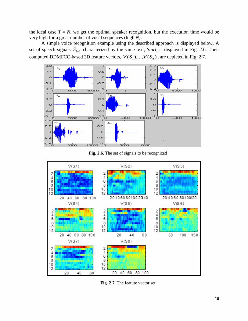
48
the ideal case T = N, we get the optimal speaker recognition, but the execution time would be
very high for a great number of vocal sequences (high N).
A simple voice recognition example using the described approach is displayed below. A
set of speech signals 81S characterized by the same text, Start, is displayed in Fig. 2.6. Their
computed DDMFCC-based 2D feature vectors, )(),...,( 81 SVSV , are depicted in Fig. 2.7.
Fig. 2.6. The set of signals to be recognized
Fig. 2.7. The feature vector set

49
The values of the distances between these vectors, ))(),(( jiij SVSVdd , are registered
in Table 2.2. One can see some of these values are low, while others are much higher One
applies the automatic feature vector clustering algorithm with these distance values, obtaining
3optK and the following voice classes: 531 ,, SSS , 72 , SS and 864 ,, SSS .
Table 2.2. Distances between vocal feature vectors
ijd 1S
2S 3S
4S 5S
6S 7S
8S
1S 0 4.32 0.98 5.09 1.67 4.88 3.87 6.11
2S 4.32 0 3.96 4.56 4.83 5.32 1.25 4.29
3S 0.98 3.96 0 3.78 0.95 5.31 5.14 6.01
4S 5.09 4.56 3.78 0 4.17 1.03 3.28 1.23
5S 1.67 4.83 0.95 4.17 0 4.61 4.11 5.87
6S 4.88 5.32 5.31 1.03 4.61 0 3.94 0.91
7S 3.87 1.25 5.14 3.28 4.11 3.94 0 4.03
8S 6.11 4.29 6.01 1.23 5.87 0.91 4.03 0
Method comparison have been also performed. We have determined that our automatic
speaker recognition technique provides comparable good results to some non-automatic
unsupervised recognition approaches, like those using Self Organizing Maps (SOMs) [44], when
applied on quite small voice sets. But when applied to medium or large sets of vocal utterances,
our method achieves much better recognition results than SOM-based approaches or other
techniques which require that speakers’ number to be known. Those methods need interactivity,
so they become very difficult to apply for large sets.
Also, we have compared the proposed automatic clustering algorithm with other voice
classification solutions. Thus, we have replaced the agglomerative hierarchical clustering region-
growing procedure with some K-means algorithms [45]. We have obtained a faster recognition
process with K-means and its variants (C-means, Fuzzy K-means) [43,45] but, unfortunately, the
obtained speaker recognition results have been considerable weaker. That means a lower
recognition rate, lower values for performance scores and more voice classification errors.
The described unsupervised voice classification technique can be used successfully to
cluster-based indexing of large speech databases, given its automatic character. The resulted
indexes, composed of feature vector clusters, would facilitate considerably the speaker retrieval
process.

50
2.2. Robust face recognition techniques
Artificial facial recognition represents a very important biometric authentication domain,
the human face being a physiological biometric identifier that is widely used in person
authentication. A facial recognition system represents a computer-driven biometric application
for automatically authenticating a person from a digital image, using the characteristics of its
face [69]. As any biometric recognition system, it performs two essential processes:
identification and verification. Facial identification consists in assigning an input face image to
a known person, while face verification consists in accepting or rejecting the previously
detected human identity. Also, the face identification is composed of a feature extraction
process and a classification procedure.
Face recognition technologies have a variety of potential applications in commerce and
law enforcement, such as database matching, identity authentication, access control for various
services, suspect recognition, information security and video surveillance [69]. Also, these
technologies can be incorporated into more complex biometric systems, to achieve a better
human recognition.
Facial recognition techniques are divided into two main categories: geometric and
photometric methods. The geometric approaches represent feature-based techniques and look at
distinguishing individual characteristics, such as eyes, nose, mouth and head outline, and
developing a face model based on position and size of these features. Photometric techniques
are view-based recognition methods. They distill a face image into values and compare these
values with templates [69].
Numerous face recognition algorithms have been developed in the last decades. The most
popular techniques include Principal Component Analysis (PCA) using Eigenfaces [70,71],
Linear Discriminant Analysis (LDA) using Fisherfaces [72], Elastic Bunch Graph Matching
(EBGM), Hidden Markov Models (HMM) [73] and the neuronal model Dynamic Link
Matching (DLM) [74].
Proposed in 1991 by M. Turk and A. Pentland [71], the Eigenface approach was the first
genuinely successful system for automatic recognition of human faces. Their model represented
a breakaway from contemporary research trend on face recognition which focused on identifying
some individual facial characteristics. I developed an eigenimage-based face recognition
technique derived from the influential work of Turk and Pentland, which is described in the next
subsection. Then, a face recognition system using 2D Gabor filtering, proposed by us, is
described in the second subsection. I also modeled an automatic unsupervised face recognition
scheme based on SIFT characteristics and a hierarchical agglomerative clustering algorithm. It is
presented in 2.2.3.
2.2.1. Eigenimage-based face recognition approach using gradient covariance
In the selected paper 3 [75] we proposed an eigenimage-based face recognition method
based on the well-known technique of Turk and Pentland [71]. Their approach considered a
large set of facial images, representing a training set. Each image was transformed into a vector
Mii ,...,1 , , then one computed the average vector Ψ . The covariance matrix was
computed next as TAAC , where MA ,...,1 and ii . The eigenvectors
and eigenvalues of C (a very large matrix) were obtained from those of AAT . Thus, TAA
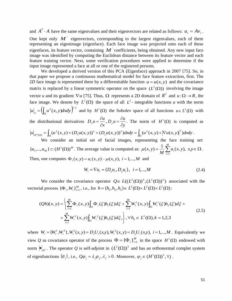
51
and AAT have the same eigenvalues and their eigenvectors are related as follows: ii Avu .
One kept only 'M eigenvectors, corresponding to the largest eigenvalues, each of them
representing an eigenimage (eigenface). Each face image was projected onto each of these
eigenfaces, its feature vector, containing 'M coefficients, being obtained. Any new input face
image was identified by computing the Euclidean distance between its feature vector and each
feature training vector. Next, some verification procedures were applied to determine if the
input image represented a face at all or one of the registered persons.
We developed a derived version of this PCA (Eigenface) approach in 2007 [75]. So, in
that paper we propose a continuous mathematical model for face feature extraction, first. The
2D face image is represented there by a differentiable function ),( yxuu and the covariance
matrix is replaced by a linear symmetric operator on the space ))(( 2 L involving the image
vector u and its gradient u [75]. Thus, represents a 2D domain of 2R and Ru : , the
face image. We denote by )(2 L the space of all 2L - integrable functions u with the norm
2/12
2),( dxdyyxuu and by )(1 H the Sobolev space of all functions )(2 Lu with
the distributional derivatives y
uuD
x
uuD yx
, . The norm of )(1 H is computed as
dxdyyxuyxudxdyyxuDyxuDyxuu yxH)),(),(())),(()),((),((
22222
)(1 .
We consider an initial set of facial images, representing the face training set:
M
M Huu ))((},...,{ 1
1 . The average value is computed as:
M
i
i x,yyxuM
yx1
),,(1
),( .
Then, one computes Miyxyxuyx ii ,...,1 ),,(),(),( and
MiuDuDuW iyixii ,...,1 },,{ (2.4)
We consider the covariance operator )))((,))((( 3232 LLLQ associated with the
vectorial process M
iii W 1},{ , i.e., for )()()(},,{ 222
321 LLLhhhh :
3,2,1),( , ,)()(),(
)()(),()()(),(),)((
2
3
1
22
2
1
11
1
1
kLhdhWyxW
dhWyxWdhyxyxQh
k
M
i
ii
M
i
ii
M
i
ii
(2.5)
where Mix,yUDyxWx,yUDyxWWWW iyiixiiii ,...,1 ),(),( ),(),( },,{ 2121 . Equivalently we
view Q as covariance operator of the process M
ii 1}{ in the space )(1 H endowed with
norm 1H . The operator Q is self-adjoint in
32 ))(( L and has an orthonormal complet system
of eigenfunctions }{ j , i.e., 0 , jjjjQ . Moreover, jHj ,))(( 31 .

52
We associate with operator Q the MM 33 matrix AAQ T~
, where 323 ))((: LRA M
M
i
i
i
M
i
i
i
M
i
i
i yWyWyAY1
3
1
1
2
1
1
1 ,, , M
i
iii yyyY 1321 },,{ and MT RLA 332 ))((: ,
which represents the adjoint operator, is provided by
dhWdhWdhWdhWdhdhhA MMM
T
3
2
3
2
12
1
2
1
1111 )(...,,)(,)(...,,)(,,...,)(
where 32
321 ))((),,( Lhhhh . We obtain:
M
jiji
ji
ji
T
d
d
d
AA
1,
00
00
00
(2.6)
We consider M
jj
3
1}{ and MM
jj R33
1}{ a linear independent system of eigenvectors for
Q~
, i.e., MjQ jjj 3,...,1 ,~
. Then, we demonstrate in [75] that M
jj
3
1}{ defined by
Mjjjj 1for , , MjMW jjj 21for ,1 , and ,2
jjj W for
MjM 312 are eigenfunctions of operator Q, i.e., MjQ jjj 3,...,1 , . It should be
recalled that the eigenfunctions }{ j to covariance operator Q maximizes the variance of
projected samples i.e.,
}1;,arg{max 3232))(())((
LLj hhQh (2.7)
In this way the eigenfunctions M
jj
3
1}{ capture the essential features of the training
images. From }{ j we keep a smaller number of eigenfaces '3
1}{ M
jj , with MM '
corresponding to largest eigenvalues j , and consider the space
323
1 ))((}{'
LlinX M
jj (2.8)
We assume that system }{ j has been normalized (i.e. orthonormal in 32 ))(( L ), so we
project any initial image 3221 ))((},,{ LWW iii on X by formula
MiTyxyxLij
M
j
ji 3,...,1 ,,),(),( 32
'
))((
3
1
(2.9)
where },,{ 21
iiii WWT Mi 3,...,1 , and 32 ))((,
L represents the scalar product in
)()()( 222 LLL [6]. We compute the weights MiTwLij
j
i 3,...,1 ,, 32 ))((
, and
model the feature vector corresponding to image iu , as following:
53
MiwwuV M
iii 3,...,1 ),,...,()('31 (2.10)
Then, the continuous model proposed in our paper is discretized. One assume that
][0, ][0, 21 LL and set 2,...1 , Niixi and 1,...1 , Njjy j , 0 . Thus one
obtains M matrices of size 21 NN , representing the discrete images, and denote their
corresponding 1 21 NN image vectors as MII ,...,1 . Also, ~
AAQ T , where
,...,00
0,...,0
00,...,
22
1
11
1
1
M
M
M
WW
WWA
(2.11)
and
12
12
12
,
1,1
2
,
1,1
1
,
1,
),(),(
),(),(
),(
NN
jijikjikk
NN
jijikjikk
NN
jijikk
yxyxW
yxyxW
yx
(2.12)
The obtained matrix has a MM 3 3 dimension. One determines the eigenvectors i of
the matrix Q~
, then, the eigenvectors of the discretized covariance operator Q are computed as:
MiA ii ,...,1 ,~ (2.13)
We keep only MM ' eigenimages corresponding to largest eigenvalues and
considered the space '3
1}~{ M
iilinspanX . Then, the projection of ],,[ 21
iii WW on X,
given by the discrete version of i , is computed as:
MiwWWPM
j
j
j
iiiiX 3,...,1 ,~]),,([
'3
1
21
(2.14)
where T
iii
T
j
j
i WWw ],,[~ 21 . So, for each facial image iI a corresponding feature vector
is obtained as MiwwIV TM
iii 3,...,1 ,],...,[)('31 . We then perform a supervised classification
process for these feature vectors. So, we consider an unknown image I to be classified using the
face training set },...,{ 1 MII .
The input image is normalized, first. So, I , where
M
i
iIM 1
1. The
vectors 1W and 2W are computed from using (2.12). Then it is projected on the eigenspace,

54
by using
'
1
~)(M
i
i
iwP , where TT
i
i WWw ] , ,[~ 21 , its feature vector being
computed as TMwwIV ],...,[)('1 [75]. A threshold-based facial test can be performed to
determine if the given image represents a real face or not. So, if TP )( , T being a
properly chosen threshold, then I is a face, otherwise it is not.
We consider K registered (authorized) persons whose faces are represented in the training
set. We redenote this set as },...,,...,,...,,...,,...,{ )(1)(1)1(
1
1
1
Kn
KK
in
ii
n IIIIII , where MK and
},...,{ )(1 in
ii II is the training subset provided by the ith authorized person. A minimum average
distance classifier, like that described in 2.1.2, is used. The input image is associated to the user
corresponding to the minimum mean distance value. That user must be the kth registered person,
where:
)(
))(),((
minarg
)(
1
in
IVIVd
k
in
j
j
i
i
(2.15)
where d is the Euclidean metric. After performing this face identification process, a face
verification is also conducted in [75]. A threshold-based face verification technique is proposed,
the proper threshold value being determined as the overall maximum distance between any two
feature vectors belonging to the same training feature subset, like in 2.1.2.
Numerous experiments, using this developed approach, have been performed on various
facial datasets, very good face recognition results being achieved [75]. We used Yale Face
Database B [76], containing thousands of 168192 facial images corresponding to many
subjects, for the tests. We found that our proposed technique achieves a high recognition rate, of
approximately 90%, and get high values for the performance parameters, Precision and Recall.
Let us describe here one of the performed face recognition experiments. In Fig. 2.8 one
can see a set of 10 input faces to be recognized. The training set, containing 30 facial images
belonging to 3 persons, is illustrated in Fig. 2.9, where each registered individual has 10 photos
positioned on 2 consecutive rows. So, one computes 90 eigenfaces for this training set but only
the most important 27 ( 9' M ) of them are required. They are represented in Fig. 2.10.
The corresponding feature vectors are then determined and the average distance values
between these input image feature vectors and the 3 feature subsets are registered in the next
table, where each row i, marked by iD , contains the distance values from the 10 feature vectors
to the ith feature subset.
It results from Table 2.3 that input images 1, 3 and 8 are identified as faces of the third
registered person from Fig. 2.8, the images 2, 6 and 10 are identified as faces of the first person
and images 4 and 7 are identified as the second person. Also, the face images 5 and 9 are
identified as belonging to the first registered person but their distance values, 5.795 and 5.101,
are greater than the computed threshold, 568.2T , so the verification procedure labels the
person with faces 5 and 10 as unregistered.

55
Fig. 2.8. Input facial images
Fig. 2.9. Face training set

56
Fig. 2.10. The main eigenfaces
Table 2.3. The mean distance values
1 2 3 4 5 6 7 8 9 10
D1 2.573 1.919 2.557 2.736 5.795 2.2702 2.108 3.147 5.101 1.923
D2 3.090 3.859 2.788 1.954 6.716 2.5956 1.789 2.623 6.959 3.467
D3 2.351 3.257 2.273 2.534 6.103 3.1354 3.293 2.331 5.143 2.926

57
2.2.2. Face recognition technique using 2D Gabor filtering
The Gabor filters are successfully used in various image processing and analysis domains,
such as: image smoothing, image coding, texture analysis, shape analysis, edge detection,
fingerprint and iris recognition. The Gabor filter (Gabor Wavelet) represents a band-pass linear
filter whose impulse response is defined by a harmonic function multiplied by a Gaussian
function. Thus, a bi-dimensional Gabor filter constitutes a complex sinusoidal plane of particular
frequency and orientation modulated by a Gaussian envelope [77]. It achieves an optimal
resolution in both spatial and frequency domains. The 2D Gabor filters have been increasingly
used in the face recognition domain, too [77,78].
I developed a supervised 2D Gabor filtering-based face recognition technique that is
described here [79]. My approach designs 2D odd-symmetric Gabor filters for facial image
recognition, having the following form:
k
kk
yxikxf
yxyxG i
yx
f 2cosexp),(2
2
2
2
,,, (2.16)
where kk yxxk
sincos , kk xyyk
sincos , if provides the central frequency of
the sinusoidal plane wave at an angle k with the x – axis, x and y represent the standard
deviations of the Gaussian envelope along the two axes, x and y. We set the phase 2/ and
compute each orientation as n
kk
, where nk ,...,1 [79,80].
The two-dimensional filters yxk fG ,,, , provided by (2.16), represent a group of wavelets
that optimally captures both local orientation and frequency information of the image. Each face
image must be filtered with yxk fG ,,, at various orientations, frequencies and standard
deviations. So, we consider some proper value for the filter parameters (variance values, radial
frequencies, orientations): 2x , 1y , 5.1 ,75.0if and n = 5, which means
,5
4,
5
3,
5
2,
5k
. So, we construct 2D Gabor filter bank ]5,1[,5.1,75.01,2,, kff
iik
G ,
composed of 10 channels [79,80].
The modelled filter set is applied to the current face, by convolving that facial image with
each Gabor filter from this set. The resulted Gabor responses are then concatenated into a three-
dimensional feature vector. If I represents a YX face image, then the proposed feature
extraction model can be expressed as:
],)[(],,)[( ,),(),( yxIVzyxIVyxzfz (2.17)
where ],1[ Xx , ],1[ Yy and
]2,1[,
],1[ ,)( ,
]2,1[,
],1[ ,)(
2
1
nnzf
nzfzf
nnz
nzz
nz
z
(2.18)
and
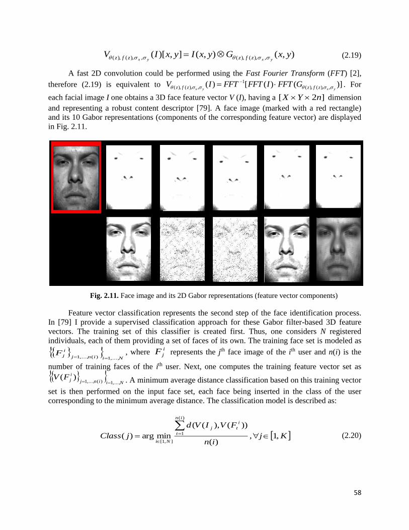
58
),(),(],)[( ,),(),(,),(),( yxGyxIyxIVyxyx zfzzfz (2.19)
A fast 2D convolution could be performed using the Fast Fourier Transform (FFT) [2],
therefore (2.19) is equivalent to )]()([)( ,),(),(
1
,),(),( yxyx zfzzfz GFFTIFFTFFTIV . For
each facial image I one obtains a 3D face feature vector V (I), having a ]2[ nYX dimension
and representing a robust content descriptor [79]. A face image (marked with a red rectangle)
and its 10 Gabor representations (components of the corresponding feature vector) are displayed
in Fig. 2.11.
Fig. 2.11. Face image and its 2D Gabor representations (feature vector components)
Feature vector classification represents the second step of the face identification process.
In [79] I provide a supervised classification approach for these Gabor filter-based 3D feature
vectors. The training set of this classifier is created first. Thus, one considers N registered
individuals, each of them providing a set of faces of its own. The training face set is modeled as
Niinj
i
jF,...,1)(,...,1
, where i
jF represents the jth face image of the ith user and n(i) is the
number of training faces of the ith user. Next, one computes the training feature vector set as
Niinj
i
jFV,...,1)(,...,1
)( . A minimum average distance classification based on this training vector
set is then performed on the input face set, each face being inserted in the class of the user
corresponding to the minimum average distance. The classification model is described as:
Kjin
FVIVd
jClass
in
t
i
tj
Ni,1,
)(
))(),((
minarg)(
)(
1
],1[
(2.20)
59
where NjClass ,1)( represents the index of the face class where input jI is introduced and
d is the squared Euclidian metric. The facial identification result, represented by the obtained
classes NCC ,...,1 , is followed by a threshold-based face verification process [79,80], modeled as:
}{)(
))(),((
:,,1
)(
1ICCT
in
FVIVd
CINi ii
in
j
i
j
i
(2.21)
where the threshold value is automatically computed as
)(),(maxmax
)](,1[
i
k
i
jinkjNi
FVFVdT .
The performed recognition experiments demonstrate the effectiveness of the described
approach [79,80]. A high face recognition rate (over 80%) is achieved by our technique, on the
basis of experiments involving hundreds frontal images. We have obtained high values for the
performance parameters, Precision and Recall. We have used Yale Face Database B, containing
thousands of 168192 facial images at different illumination conditions, representing various
persons, for our recognition tests [76]. While we obtain very good recognition results for frontal
faces, considerable lower recognition rates are achieved for images representing rotated or non-
frontal faces.
Method comparisons have been also performed. The performance of this approach has
been compared with those of Eigenface-based systems. We have tested the Eigenface algorithm
of Turk & Pentland [71], the Eigenface method proposed by us [79] and this Gabor filter based
technique, on the same face dataset. The values of statistical parameters Precision and Recall,
computed for these algorithms, are registered in Table 2.4. As one can see in this table, the three
face recognition techniques provide comparable good results. The original Eigenface-based
technique performs slightly better than our two methods.
Table 2.4. Performance parameter comparison
A face recognition example is described next. A small facial training set, composed of the
faces of three authorized persons, is represented in Fig. 2.12. A small sized input image set, with
K = 6, is displayed in Fig. 2.13. The computed average distance values are registered in Table
2.5.
From this table, it results the following face identification: User 1 => 42 , II , User 2 =>
51, II , User 3 => 63 , II . We also compute T = 0.9759, so, the face verification provides the
final recognition result: User 1 => 42 , II , User 2 => 1I , User 3 => 63 , II , Unregistered =>
5I .
Eigenface (T&P) Eigenface (Barbu) Gabor filter based method
Precision 0.95 0.85 0.88
Recall 0.94 0.85 0.90

60
Fig. 2.12. Face training set
Fig. 2.13. Input face set
Table 2.5. Resulted average distance values:
1I 2I
3I 4I
5I 6I
User 1 1.0970 0.6208 1.5475 0.7779 1.6175 1.0379
User 2 0.5581 1.4291 1.7623 1.2103 1.1313 1.2551
User 3 1.2154 1.0946 0.9278 1.2548 1.3562 0.6333

61
2.2.3. Automatic unsupervised face recognition system
In the previous subsections we described two supervised facial recognition techniques that
work properly for cooperative human subjects, being very useful for access control. Now we
describe an unsupervised face recognition method that could deal with non-cooperative subjects
and can be successfully used by the surveillance systems [51].
Most of the existing face authentication techniques perform the recognition in a supervised
manner, but numerous unsupervised methods have been developed recently. Thus, we mention
the SOM-based face recognition techniques [81], the unsupervised methods based on PCA or
ICA (Independent Component Analysis) [82], and the unsupervised face recognition by
associative chaining [83]. We modeled an unsupervised facial recognition system having also an
automatic character [37].
In [37] we considered the following unsupervised recognition task. The set of faces
{𝐹1, … , 𝐹𝑛} must be clustered automatically, on the similarity basis. The faces from each resulted
cluster have to belong to the same person. Because of the unsupervised character of the process,
the persons are unknown and no facial training set is available. Even the number of these persons
is unknown, given the automatic character of the process.
A robust SIFT-based facial feature extraction is performed on iF images [37]. Published
by David Lowe in 1999, Scale Invariant Feature Transform represents a computer vision
algorithm that locates and describes local image features [84]. SIFT characteristics are widely
used in computer vision areas like object tracking and recognition. The SIFT algorithm
determines the main keypoints from the image to produce a proper feature description. The
extracted features are invariant to scaling, orientation, affine transforms and illumination changes
[84], so they are well-suited for face description.
The SIFT characteristics of a face image are obtained in several steps. First, one computes
the maxima and minima values of the result of Difference of Gaussians (DoG) filters applied at
different scales on the face image. Then, the low contrast points are discarded. A dominant
orientation is then assigned to each of the identified keypoints. For each keypoint one computes a
local feature descriptor on the basis of the local image gradient, transformed according to
keypoint orientation to obtain orientation invariance. So, one obtains a SIFT feature vector of
128 coefficients for each face keypoint. The face feature vector corresponding to iF is modeled
as follows:
)(
...
)(
,
)(
...
)(
)(
11
in
i
in
i
i
Floc
Floc
Fv
Fv
FV
ii
(2.22)
where )( ik Fv is the feature vector of the kth keypoint of iF and )( ik Floc is a pair of coordinates
representing its location in the face image [37]. The keypoints are positioned in the feature vector
given by (2.22) from left to right and from top to the bottom. Since )( iFV
represent complex
feature vectors, the distances between them could not be measured using the Euclidean metric or
other conventional metrics. So, the special metric introduced in subsection 1.4.2 is used for this
purpose [37]. The set of matches used by that metric and given by (1.53) is replaced in this case
with:

62
21 ))(),((&))(),((|, TFlocFlocdTFvFvdtkM jtikEjtikEij (2.23)
where the threshold values 1T and 2T are detected empirically, and Ed
represents the Euclidean
metric.
The face feature vector classification is performed in [37] by applying the validity index-
based automatic clustering model described in 1.4.4 on the feature set { )( iFV }i=1,…n. The
clustering algorithm used repeatedly in that model is now a hierarchical agglomerative one that
computes the distance between clusters using the average linkage clustering approach, and the
distances between facial feature vectors are computed using (1.52) and (2.23).
The described unsupervised facial recognition method has been tested on the same Yale
Face Database B, containing thousands of 192 × 168 faces, used in the previous cases [76]. A
high face recognition rate, of approximately 90%, is obtained, being influenced also by the
threshold value selection. The optimal values used in (2.23) are 65.01 T and 152 T . High
performance parameters values have been also achieved: Precision = 0.93, Recall = 0.91 and F1
= 0.92. These values prove that our recognition technique produces very few missed hits and
very few false positives.
An unsupervised face recognition example is described next. Image set displayed in Fig.
2.14 contains 8 faces, 81 ,..., FF , belonging to 3 persons (2 males, 1 female). Face feature vectors,
)( 81FV , are obtained from (2.22). The automatic clustering process is applied, resulting the
optimal number of clusters 3optimK and the final recognition result: 8611 ,, FFFC , 422 , FFC
and 7533 ,, FFFC . These classification results are displayed in Fig. 2.15, each row of it
containing the faces from a class and their SIFT characteristics: keypoints and their orientations.
Fig. 2.14. The set of faces to be recognized

63
Fig. 2.15. SIFT characteristics and face clustering result
Method comparison was also performed [37]. Because of its automatic character, the
proposed recognition technique executes much faster and provides better results for large face
sets than non-automatic approaches. Also, our SIFT-based method produces better recognition
results than unsupervised techniques using other face features, such as Eigenfaces [70,71] or 2D
Gabor filtering based characteristics [78,79]. We also considered some other versions of the
automatic classification algorithm. Thus, we tested it with various K-means algorithms [45] and
Self-Organizing Feature Maps (SOFM) [81], instead of the region-growing procedure, on the
same face feature sets, but achieved weaker recognition results and also slower execution times.
The performance parameters of several face recognition techniques are registered in the
next table. One can see their values for this SIFT-based unsupervised method, the PCA
(Eigenface) algorithm [70,82], the ICA-based technique [82], unsupervised version of Barbu’s
2D Gabor filtering approach [80], and an algorithm using SIFT characteristics with K-means
clustering. As it results from Table 2.6, the recognition technique provided here achieves the
highest values for Precision, Recall and F1, which means it outperforms the other approaches.
Table 2.6. The performance parameters for several face recognition approaches
This method Eigenface (PCA) ICA Unsupervised
Gabor filter-based
SIFT/K-means
Precision 0.93 0.92 0.90 0.88 0.88
Recall 0.91 0.90 0.88 0.86 0.91
F1 0.9199 0.9099 0.8899 0.8699 0.8947

64
The recognition techniques measured by performance parameters registered in Table 2.6
have been tested on hundreds [192 × 168] faces of Yale Face Database B. Their corresponding
RPC (Recall versus Precision Curves) are displayed in Fig. 2.16. The RPC of our model, marked
in blue, also proves its performance.
Fig. 2.16. RPC curves for several face recognition approaches
Because of its automatic and unsupervised character, the facial recognition technique
described here can be successfully applied not only for non-cooperative subjects in video
surveillance systems [85], but also for voluminous face sets. So, an important application area of
our unsupervised recognition approach is face database indexing and retrieval. Some robust
clustering-based face indexing methods [86] can be developed using our face recognition system.
2.3. Person authentication via fingerprint recognition
The fingerprint represent one of the most known forms of biometrics used to authenticate
human persons. Because of their uniqueness and consistency over time, fingerprints have been
used for person recognition for over a century [87].
Fingerprint recognition represents the computerized automated process of determining the
identity of an individual using the characteristics of his fingerprints. Obviously, a fingerprint
recognition system is a biometric authentication system that performs two main operations:
fingerprint identification and verification. Fingerprint identification associates each input
fingerprint with a registered user of the system, consisting of a fingerprint feature extraction and
a feature vector classification. Fingerprint verification represents the task of validating the
associated identity of a fingerprint, usually using proper threshold values.
The main application area of fingerprint recognition systems is law enforcement. Another
important application field of fingerprint authentication is access control to various services,
numerous security systems being based on fingerprints [88].
The fingerprint recognition approaches are divided into two major categories: minutiae-
based [89] and pattern-based techniques [90]. We developed recognition methods from both
65
categories. Thus, a robust minutiae-based fingerprint authentication model is described in the
next subsection. Then, a pattern-based fingerprint recognition technique using 2D Gabor filters is
presented in 2.3.2. Another pattern-based recognition approach, but based on 2D Wavelet
Decompositions, is described in the last subsection.
2.3.1. Minutiae-based fingerprint authentication approach
The fingerprint is composed of ridges and valleys. The minutia points represent unique
features found within the fingerprint patterns. There are various types of minutia details such as:
ridge endings, bifurcations, short ridges, dots, crossovers, spurs and islands [38,89]. The most
important fingerprint points are the ridge endings, short ridges and bifurcations.
Most modern fingerprint recognition technologies are based on minutiae matching [89].
The idea of minutiae-based matching is if one can find enough minutiae in one image that have
corresponding minutiae in another image, then those images are most likely from the same
fingerprint. The most commonly used minutiae points by the existing fingerprint recognition
approaches are the ridge endings and bifurcations. Any minutiae-based fingerprint recognition
technique performs a minutiae detection process before minutiae matching.
We proposed several minutiae based recognition methods in our past works [38,53,91].
The same minutiae detection procedure was performed by each of them. First, a fingerprint
image enhancement process, consisting of denoising and restoration operations, was applied.
While there exist some direct minutiae extraction techniques that identify the fingerprint minutia
points by following the ridge line in the grayscale image of the fingerprint [92], we considered a
binarization-based solution. The enhanced image was converted from grayscale to the binary
format using a thresholding algorithm.
Fig. 2.17. Minutiae detection process
66
Then, the skeletonization, performed using a thining algorithm, produced the
morphological skeleton of the binary image of the fingerprint [93]. Image thinning represents a
morphological process that is similar to erosion and opening and produces very thin ridges,
having a width of one pixel [93]. The most popular thinning algorithms are medial axis method,
contour generation method, local thickness based thinning approach, sequential and parallel
thinning [94].
The thinned ridges facilitated the fingerprint minutiae detection task. We considered 8 –
neighborhoods of black pixels in this identification process. For each black pixel (0 value) of the
skeleton, one determined if it represents either a minutia point or an ordinary pixel. The detection
algorithm counted the number of neighbours of the current black pixel. There could be three
possible situations. If the pixel has only one neighbour, then it represents a ridge ending. If the
pixel has at least 3 neighbours, then it represents a bifurcation. If the pixel has 2 neighbours, then
it is an intermediary pixel. A minutia point detection process is described in Fig. 2.17.
The identification process is followed by the minutiae matching. In [91] we develop some
minutiae-based fingerprint matching approaches based on neural networks. The modeled NN-
based classifiers operated on minutiae-based feature vectors obtained using some Zernike
moments. We will not insist on those NN-based recognition techniques here, describing the most
recently developed fingerprint matching approach instead.
So, in selected paper 4 (Barbu 2011[38]) we introduce a robust fingerprint recognition
system based on minutia point matching. In its feature extraction stage, one models the
fingerprint feature vector on the basis of the feature vectors corresponding to the detected
minutiae [38]. The sequence of the minutia points identified in the fingerprint F is noted as
F
Fm
F MM )(1 ,..., . The fingerprint feature extraction process is modeled as follows:
)(),...,()( )(1
F
Fm
F MVMVFV (2.24)
where )( F
iMV represents the feature vector of F
iM , )(,1 Fmi . Each of these vectors contains
the essential information related to the corresponding minutia: its type (ridge ending,
bifurcation), its position (provided by coordinates) and its orientation, representing the angle of
the minutia tangent and orizontal axis [89,95]. So, the feature vector of a fingerprint minutia is
constructed as:
F
i
F
i
F
i
F
i
F
i yxTypeMV ,,,)( (2.25)
where F
iType represents the minutia type of F
iM , F
ix and F
iy are its coordinates, and F
i
represents the orientation of F
iM . These measures of a minutia, which compose the feature
vector, are represented in Fig. 2.18.
From relations (2.24) and (2.25) we determine the final form of the feature vector of
fingerprint F:
F
Fm
F
Fm
F
Fm
F
Fm
FFFF yxTypeyxTypeFV )()()()(1111 ,,,,...,,,,)( (2.26)
67
Fig. 2.18. The minutiae used in the matching process
The components F
iM are arranged in the sequence corresponding to F in the order given
by their coordinates. They were aligned from left to right and from top to the bottom, as follows:
F
i
F
i
F
i
F
i
F
Fm
F
i
F
yyxx
xxx
11
)(1 ....... (2.27)
Obviously, the fingerprint feature vectors computed by (2.26) represent complex
structures that cannot be classified using conventional metrics. We use the special metric
described in 1.4.2 to measure the distances between these feature vectors [38]. The metric given
by (1.52) took in this case the next form:
))(),((2
)()())(),(( 21
2121 FVFVp
FmFmFVFVd
(2.28)
where
21212121
112121 ,,,)(),(min))(),((FFF
i
F
i
F
i
F
i
F
i
F
i yyxxTypeTypeFmFmicardFVFVp (2.29)
Then, a supervised fingerprint classification is performed, using the minimum average
distance classifier [38] or the K-NN [61]. So, we may consider a set of input fingerprint images
},...,{ 1 nFF to be authenticated. We model a training set composed of templates representing the
fingerprints of N registered individuals. The training set is obtained as Niinj
i
jT,...,1)(,...,1
, each
i
jT being the jth template of the ith registered user. Each fingerprint is associated to the
registered user corresponding to the minimum average distance between the fingerprint’s feature
vector and the training vectors of that user. Thus, the class of the current input fingerprint results
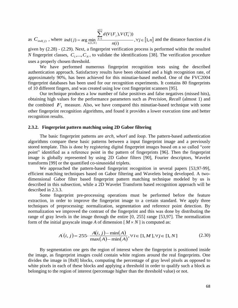
68
as )( jindC , where njin
TVFVd
jind
in
k
i
kj
Ni,1,
)(
))(),((
minarg)(
)(
1
],1[
and the distance function d is
given by (2.28) - (2.29). Next, a fingerprint verification process is performed within the resulted
N fingerprint classes, NCC ,...,1 , to validate the identifications [38]. The verification procedure
uses a properly chosen threshold.
We have performed numerous fingerprint recognition tests using the described
authentication approach. Satisfactory results have been obtained and a high recognition rate, of
approximately 90%, has been achieved for this minutiae-based method. One of the FVC2004
fingerprint databases has been used for our recognition experiments. It contains 80 fingerprints
of 10 different fingers, and was created using low cost fingerprint scanners [95].
Our technique produces a low number of false positives and false negatives (missed hits),
obtaining high values for the performance parameters such as Precision, Recall (almost 1) and
the combined 1F
measure. Also, we have compared this minutiae-based technique with some
other fingerprint recognition algorithms, and found it provides a lower execution time and better
recognition results.
2.3.2. Fingerprint pattern matching using 2D Gabor filtering
The basic fingerprint patterns are arch, whorl and loop. The pattern-based authentication
algorithms compare these basic patterns between a input fingerprint image and a previously
stored template. This is done by registering digital fingerprint images based on a so called “core
point” identified as a reference point in the pattern of fingerprints [96]. Then the fingerprint
image is globally represented by using 2D Gabor filters [90], Fourier descriptors, Wavelet
transforms [99] or the quantified co-sinusoidal triplets.
We approached the pattern-based fingerprint recognition in several papers [53,97-99],
efficient matching techniques based on Gabor filtering and Wavelets being developed. A two-
dimensional Gabor filter based fingerprint pattern matching technique modeled by us is
described in this subsection, while a 2D Wavelet Transform based recognition approach will be
described in 2.3.3.
Some fingerprint pre-processing operations must be performed before the feature
extraction, in order to improve the fingerprint image to a certain standard. We apply three
techniques of preprocessing: normalization, segmentation and reference point detection. By
normalization we improved the contrast of the fingerprint and this was done by distributing the
range of gray levels in the image through the entire [0, 255] range [53,97]. The normalization
form of the initial grayscale image A of dimension [ NM ] is computed as:
],1[],,1[,minmax
min,255,' NjMi
AA
AjiAjiA
(2.30)
By segmentation one gets the region of interest where the fingerprint is positioned inside
the image, as fingerprint images could contain white regions around the real fingerprints. One
divides the image in [8x8] blocks, computing the percentage of gray level pixels as opposed to
white pixels in each of these blocks and applying a threshold in order to qualify such a block as
belonging to the region of interest (percentage higher than the threshold value) or not.

69
The reference point, or core point, of the fingerprint, used as the center of the feature map
corresponding to the fingerprint, is detected as the point where the curvature of the fingerprint
ridge is the most accentuated [53,90]. We construct an orientation map of all ridges in the
fingerprint image and then on this map one detects the pixels for which their orientation is more
different than the one of its neighbors [90,97].
As we have already mentioned, the 2D Gabor filtering represents a very useful tool for
many areas of image processing and analysis. We use it here to extract global and local features
of the fingerprint valleys and ridges. These two-dimensional filters capture local orientation and
frequency information, very useful in characterizing fingerprint patterns [90]. We model an even
symmetric 2D Gabor filter, given by:
i
ii
yxifx
yxyxG
yx
f
2cosexp,2
2
2
2
,,,
, (2.31)
where ii yxxi
sincos and ii xyyi
sincos [53, 98]. The parameter f is determined
in relation with the frequency of the ridges, which corresponds to the average distance between
the ridges. For a 500 dpi image, the average distance between ridges is 8 pixels, hence we
considered the value 125.08/1 f . We also set x = y = 4 as a compromise between the
robustness to noise and the filtering precision [98]. We also consider 8 orientations for filtering,
therefore }5,157,135,5,112,90,5.67,45,5.22,0{},...,{ 81
. The fingerprint image
is filtered by convolution with the modeled 2D Gabor filter set, for the 8 considered orientations.
Due to performance reasons, the results of the Gabor filtering cannot be used directly as
feature vectors. Instead, the Gabor filtered image is processed through a grid centered in the core
point of the fingerprint [53]. That rectangular grid is composed of [10 x 10] cells, each cell
having 16 by 16 pixels.
Fig. 2.19. Rectangular grid applied to fingerprint (L), Gabor filtered fingerprint (C), feature map (R)

70
For each rectangular cell we calculate the standard deviation of the filtered fingerprint,
which corresponds to the local energy of the Gabor filter response [53]. The collection of
standard deviation values extracted from the grid forms a feature map for the fingerprint. There
are obtained 8 such feature maps, one for each orientation. In Fig. 2.19 one can see the applied
grid, the filtering result and the obtained feature map.
On the basis of these feature maps, we create a tridimensional feature vector for each
fingerprint [53,98]. Therefore, for the analyzed fingerprint A, its 3D feature vector is modeled as
follows:
]8,1[,,, iAHiyxAV i (2.32)
where AH i is the feature map of fingerprint A corresponding to the i orientation of the
Gabor filter defined by (2.31). To measure the distance between two such feature vectors, the
sum of absolute differences (SAD) between the vector components is used as a metric.
This pattern feature extraction is followed by a supervised classification of these 3D
fingerprint feature vectors. The input fingerprints {A1,…, An} are classified using a training set of
fingerprints Niinj
i
jAmp ,...,1,...,1 }}{{ corresponding to N registered persons, like in the minutiae-
based recognition case. Each fingerprint Aj has to be inserted into the fingerprint class Cind(j),
where
nj
in
AmpVAVd
jind
in
n
i
nj
Ni,1,
,
minarg 1
,1
and function d is the SAD metric. The
fingerprint verification process is performed using the already described threshold-based
algorithm, the proper threshold value being detected automatically, as in (2.3).
A lot of fingerprint recognition experiments have been performed using the proposed
approach, satisfactory results being obtained. The described recognition method has been applied
to a database of 140 fingerprint images of 300 by 600 pixels including multiple images selected
for each finger of 5 individuals. The experiments produced an authentication rate of over 80%.
Using a larger number of orientations for the Gabor filters can increase the recognition rate
of our technique at the expense of computational time. The complexity of the 2D Gabor filtering
in one direction is of the order O(n), as it is normalization and segmentation, while the detection
of the reference point has a complexity of O(n2).
2.3.3. Pattern-based fingerprint recognition using 2D Wavelet Decomposition
The wavelet features are used by certain minutiae-based recognition techniques. While
minutiae-based fingerprint authentication uses both 1D and 2D wavelet analysis [100], the
pattern based fingerprint recognition uses the two-dimensional wavelet transforms only [101,
102]. In [99] we proposed a fingerprint authentication technique based on 2D – DWT.
The 2D Discrete Wavelet Transform (2D DWT) represents a multi-resolution analysis
technique for two-dimensional signals. Applying a multi-level 2D DWT decomposition on a
digital image produces its conversion from the spatial domain into the frequency domain, while
providing a series of sub-images known also as sub-bands [101]. The implementation of the
Discrete Wavelet Transform is performed by using two filters for 2D signal processing: a low-
pass filter and a high-pass filter. The discrete wavelet analysis passes the two-dimensional signal
through these two complementary filters, the result of this processing being two 2D distinct
71
signals. The first filter extracts the low frequency components, the most important ones, known
as approximations of the 2D signals. The second one extracts the high frequency components,
known as the details of such signals. In Fig. 2.20 one describes the block diagram of the
decomposition of a two-dimensional discrete signal S on the basis of these two types of digital
filters. The two resulted component signals are A, containing the approximations of signal S,
respectively D, containing the details of the same signal [53,99]. The decomposition process may
continue iteratively on several levels, the approximations’ component signal, A, being the one
reprocessed through DWT. At each level the approximations’ signal is filtered and decomposed
in the two 2D signals of lower resolution, and so on.
Fig. 2.20. Wavelet decomposition of a signal
The wavelet decomposition tree corresponding to an image I is schematically represented
in Fig. 2.21. In the next figure one can see 3 decomposition levels.
Fig. 2.21. DWT decomposition tree of the digital image I
72
We applied such DWT decompositions in the process of their recognition. In Fig. 2.21
there is represented an example of Discrete Wavelet Transformation on 4 levels for a fingerprint
image.
Fig. 2.22. DWT decomposition of a fingerprint
The preprocessing operations described in 2.3.2 are performed in this case, too. The most
important of them is reference point detection. After preprocessing stage one models a feature
vector on the basis of the wavelet characteristics of the preprocessed image. In our approach
[99], we cut a NM rectangular region inside the fingerprint F, centered on the identified
reference point. Resulted image was then divided into non-overlapping KK blocks [99].
For each iB from the sequence of resulted blocks nBB ,...,1 , we apply the multi-
resolution 2D-DWT analysis down to the k level. So, we start with i
i BA 0 , and on each level j
the current block i
jA 1
is decomposed in the sub-images i
jA and i
jD , corresponding to
approximations and details. From here on we take into consideration only the sub-images
corresponding to the resulted details, i
k
i DD ,...,1 , for each of them computing the normalized
energy. The obtained sequence of the k values is considered as the feature vector of the block iB .
The feature vector of the fingerprint results by concatenating the vectors belonging to each
component block, and this is done by placing them on the rows of a matrix [53,99]. The model of
the wavelet-based feature extraction for the F fingerprint image is given by:
kjnijBVjiFV i ,1,1, ,)(,)(
(2.33)
where
kjni
D
DjBV
k
t
i
t
i
j
i ,1,,1,)(
12
2
(2.34)
and 2
represents the Euclidean norm of the signal taken as an argument [53,99].
73
The 2D fingerprint feature vector V(F) resulted from (2.33), has a kn dimension and
a high discrimination power between fingerprints because it approximates the energy of the
fingerprint image on several levels. The distances between these fingerprint feature vectors can
be measured using the Euclidean distance (and its variants) or SAD.
The fingerprint identification is performed by applying a similar minimum average
distance based supervised classification procedure to these DWT-based feature vectors [99]. A
K-NN feature vector classification could also be performed in this case. A threshold-based
fingerprint verification operation is performed next, to validate the identifications [53,99].
The pattern-based authentication technique described here has been tested on many
fingerprint datasets. The numerous performed experiments produced satisfactory results. A high
fingerprint recognition rate, of approximately 85%, has been achieved and also high values have
been obtained for Precision and Recall parameters. The same database as in the previous case,
containing 140 fingerprint images of size [300 x 600], including 10 images per finger of 5
individuals, has been used for these tests. These images have been selected from database based
on the fingerprint pattern inside the image, being preferred those having the reference point
located close to image center. The poor quality images or those having the core point too close to
their margins have been rejected. The reference point detection process executes quite fast, its
execution taking approximately 1.5 seconds. The detection algorithm has a complexity of O(n2).
2.4. Multi-modal biometric technologies
The unimodal biometric systems must deal with various problems, such as the noisy
biometric data, intra-class variability, inter-class similarity, restricted degrees of freedom, non-
universality, spoof attacks and unacceptable error rates. Multimodal biometrics was introduced
to address some of these limitations [103].
A multimodal biometric system can be understood in various ways. Thus, one
distinguishes the following multimodal biometric system categories: multi-sensor systems, which
have multiple sensors (optic, chip-based, ultrasound-based and others); multi-method systems,
using multiple feature vector classification techniques; multi-sample systems, using various
samples of the same identifier; multi-characteristic systems, using data from multiple biometric
identifiers [103].
The architecture of a generic biometric system consists of four main modules: sensor
module, feature extraction module, matching (classification) module and decision (verification)
module. Biometric information fusion represents an important process performed within a
multimodal biometric system. The information fusion can occur in any of the mentioned modules
[103,104]. The fusion at the sensor level consists of fusing the biometric data originating from
multiple sources (sensors). The fusion at the feature extractor level unifies the feature vectors
computed for multiple identifiers. Classifier level fusion consists of combining the results
generated by more classifiers. The decision level fusion combines the obtained authentication
decisions using techniques like that based on majority vote [103,104].
Obviously, performing the integration of the biometric information at the first levels would
produce optimal recognition results, because the feature set contains more information about
input data than the matching score or the output decision. Unfortunately, the low level fusion is
difficult to achieve because of incompatibilities between feature vectors corresponding to
different biometric identifiers. Also, the fusion at the decision level is considered too rigid due

74
to the availability of limited information. For this reason, the fusion is performed more often at
the matching module level [103,104].
Combining multiple classifiers can be performed using fusion techniques such as simple
sum rule [105], HyperBF networks [106], Borda count based methods [107], and other
approaches [103,104]. The fusion strategies at the decision level include, besides the already
mentioned majority voting, the behavior knowledge space method [108], the AND/OR rules
[109] and weighted voting based on Dempster-Shafer theory of evidence [110].
In our 2012 book we provided an overview of the multimodal biometrics. Also, we
considered multimodal biometric systems based on the three biometric identifiers (voice, face
and fingerprints) and their corresponding authentication techniques [53]. Various multimodal
biometric systems could be developed using voice, face and fingerprints [111], or combinations
of two of the three biometrics. Thus, there exist numerous bimodal systems based on speech and
face [112], voice and fingerprint [113], or face and fingerprint [114].
We have combined the unimodal biometric systems described in the previous sections of
this chapter to obtain more complex multimodal recognition systems. Thus, in [91,115] we
describe some multimodal biometric systems based on voice, face and fingerprint recognition
methods. Our multi-characteristic systems contain some text-dependent voice authentication
components based on the described DDMFCC-based speech analysis. The facial recognition is
performed by using parts-based representation methods and a manifold learning approach. The
fingerprint recognition performed within these systems is approached by minutiae detection and
matching technique using neural networks [91]. The biometric information fusion is applied at
the decision level, the final decision being taken by using a majority voting technique applied to
the three biometric identifiers [91,115]. The developed multimodal biometric authentication
approach achieved a high person recognition rate, of about 92%.
Fig. 2.23. Bimodal biometric system based on voice and face identifiers
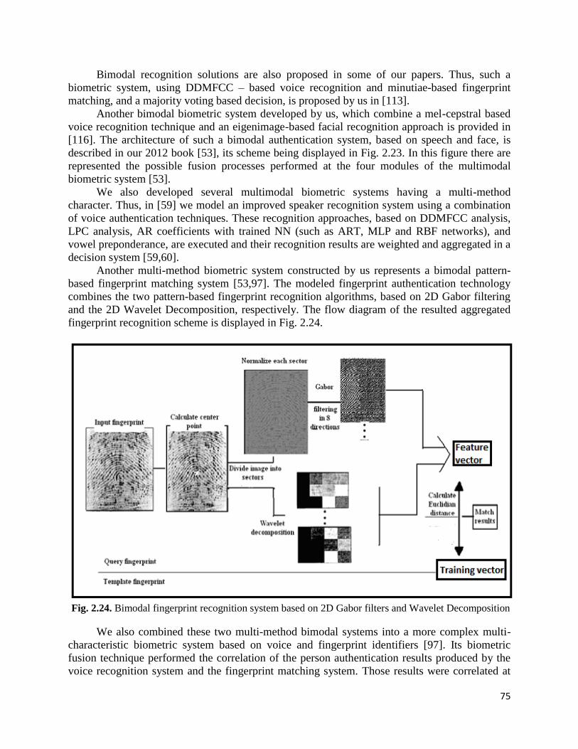
75
Bimodal recognition solutions are also proposed in some of our papers. Thus, such a
biometric system, using DDMFCC – based voice recognition and minutiae-based fingerprint
matching, and a majority voting based decision, is proposed by us in [113].
Another bimodal biometric system developed by us, which combine a mel-cepstral based
voice recognition technique and an eigenimage-based facial recognition approach is provided in
[116]. The architecture of such a bimodal authentication system, based on speech and face, is
described in our 2012 book [53], its scheme being displayed in Fig. 2.23. In this figure there are
represented the possible fusion processes performed at the four modules of the multimodal
biometric system [53].
We also developed several multimodal biometric systems having a multi-method
character. Thus, in [59] we model an improved speaker recognition system using a combination
of voice authentication techniques. These recognition approaches, based on DDMFCC analysis,
LPC analysis, AR coefficients with trained NN (such as ART, MLP and RBF networks), and
vowel preponderance, are executed and their recognition results are weighted and aggregated in a
decision system [59,60].
Another multi-method biometric system constructed by us represents a bimodal pattern-
based fingerprint matching system [53,97]. The modeled fingerprint authentication technology
combines the two pattern-based fingerprint recognition algorithms, based on 2D Gabor filtering
and the 2D Wavelet Decomposition, respectively. The flow diagram of the resulted aggregated
fingerprint recognition scheme is displayed in Fig. 2.24.
Fig. 2.24. Bimodal fingerprint recognition system based on 2D Gabor filters and Wavelet Decomposition
We also combined these two multi-method bimodal systems into a more complex multi-
characteristic biometric system based on voice and fingerprint identifiers [97]. Its biometric
fusion technique performed the correlation of the person authentication results produced by the
voice recognition system and the fingerprint matching system. Those results were correlated at
76
the decision module level, using a weighted inference system based on Dempster-Shafer
evidence theory [97].
Combining multiple biometrics and biometric recognition approaches could enhance
considerably the performance and accuracy of the human authentication process. Our multimodal
biometric systems achieve much better recognition results and obtain higher recognition rates
than each of their unimodal authentication components.
Our biometric authentication could be improved further by adding new identifiers and
algorithms. Thus, we intend to obtain more satisfactory results in the iris recognition subdomain
[54,117], such that to successfully include the person authentication techniques based on this
biometric identifier (iris) into much more complex multimodal biometric systems that make also
use of speech, face and fingerprint biometrics.
2.5. Conclusions
We have conducted extensive research in the biometrics domain in the last ten years. The
most important research results, disseminated in 25 scientific publications (books, chapters,
articles published in international journals and conference proceedings) have been described in
this chapter. We brought important contributions to this research field, developing many
unimodal and multimodal person authentication techniques based on various biometric
identifiers.
The most reliable biometric recognition results were obtained for three identifiers: voice,
face and fingerprints. We performed three types of tasks in this area: development of unimodal
biometric systems; modeling unsupervised person recognition approaches; development of
multimodal biometrics technologies. Each unimodal biometric system being based on a
supervised recognition technique involving a single identifier, we developed several supervised
voice, face and fingerprint recognition models that outperform existing approaches.
While most speaker recognition systems use same-sized 1D vocal feature vectors, our
proposed (text-dependent) voice recognition models compute robust different-sized 2D feature
vectors through an original DDMFCC-based voice analysis. Since conventional metrics do not
work for these speech feature vectors, we have created the Hausdorff-derived metric described in
previous chapter, especially for them. While the eigenimage-based face authentication system
represents our main contribution in the face recognition domain, the 2D Gabor filter-based facial
recognition technique constitutes another original contribution, too. We also developed some
novel and effective fingerprint recognition systems. The complex minutiae-based fingerprint
feature vectors, modeled by our minutia matching system and classified by using a special
metric, represent our most important contribution in this field. We also constructed pattern-
matching based fingerprint recognition models using feature vectors obtained from 2D Gabor
filter-based and 2D-DWT based feature extractions. All these biometric authentication systems
perform supervised feature vector classification processes that use a minimum average distance
classifier developed by us, besides the well-known K-NN classifier.
The proposed unsupervised biometric recognition methods, representing also important
contributions, are based on voice and face identifiers and use the validity-index based automatic
clustering algorithms developed by us. The special metrics constructed for the DDMFCC-based
2D voice feature vectors and the SIFT-based face feature vectors are applied in the clustering
processes. Because of their automatic character, these unsupervised person recognition
approaches could be used successfully for indexing voluminous voice and face databases, by

77
constructing speaker and face cluster-based indexes. Some unsupervised biometric recognition
models based on fingerprints can also be developed, by applying our automatic clustering
procedures to minutia-based or pattern-based fingerprint feature vectors.
We also developed some effective multimodal biometric solutions based on various
combinations of voice, face and fingerprints or various combinations of biometric authentication
techniques. These multi-characteristic and multi-method biometric systems produce enhanced
person recognition results. Usually, our multimodal person authentication techniques perform the
biometric information fusion at the classifier or decision level. The fusion at lower levels will be
investigated during our future research in multimodal biometrics domain.
Some part of my research in the biometrics field has been only mentioned and not
described in this thesis. For example, our iris recognition and text-independent voice recognition
results were not described here. This is due to space reasons, since this part of the thesis is
limited to a number of characters, and also because I am not satisfied enough with these results
and intend to further improve those recognition techniques in the future.

78
3. Image analysis based computer vision models
The goal of the computer vision domain is to duplicate the human vision. It includes real-
world image and video acquiring, processing, analyzing and interpretation techniques in order to
produce representation of objects in the world [118]. Computer vision field has important
applications in several strongly related domains such as artificial intelligence, robotics and
human-computer interaction. Digital signal processing is also closely related to computer vision,
but mainly through its 2D signal processing and analysis techniques. While unidimensional
signals are rarely used in computer vision applications, image analysis represents the most
closely related field to computer vision.
A typical computer vision system performs an image/video acquisition process first, using
its sensors, then it executes some pre-processing operations on the acquired data, such as image
denoising/restoration or contrast enhancement. Next, certain image and video analysis tasks are
performed by the system. Some typical tasks of a computer vision system include image
reconstruction, object and event detection, motion estimation, video tracking, object and action
recognition, learning, or content-based indexing and retrieval.
We have investigated most of these computer vision domains, the image analysis
techniques related to them and developed by us being described in the following sections of this
chapter. The image segmentation field is approached in the next section, where our region-based
and contour-based segmentation solutions are described, while the video segmentation domain is
described in 3.2, where our automatic temporal video segmentation technique is presented.
Image reconstruction, or inpainting, is approached using some robust variational PDE models
that are detailed in the third section. In 3.4 we consider the object recognition domain, presenting
some methods of recognizing objects from digital images and video sequences. Multimedia
information indexing and retrieval, another important computer vision area, is considered in
section 3.5, where we describe some content-based media indexing and retrieval techniques
developed by us. In the last section of this chapter, our proposed image and video object
detection and tracking approaches are presented.
3.1. Novel image segmentation techniques
Image segmentation represents an important image analysis domain that is useful to many
other computer vision fields. The segmentation refers to the process of partitioning a digital
image into multiple segments, or regions, which represent sets of pixels [118]. All the pixels in a
region are similar with respect to some characteristic or computed property, such as color,
intensity, or texture. Obviously, image object detection constitutes the main application area of
image segmentation.
The image segmentation algorithms can be classified into two major categories: region-
based and contour-based techniques. Region-based methods provide a set of regions that
collectively cover the entire image. They include histogram-based [119], clustering based [120],
graph partitioning based [121], watershed based and neural network based techniques. The
contour-based segmentation approaches provide a set of contours extracted from the image. Most
of them use edge detection filters [122], partial differential equation-based models [123] or
active contours (snakes) for the segmentation process [124].
Region-based image segmentation domain is approached in the next subsection. We
developed some robust region-based segmentation techniques using pixel clustering, which are

79
described in 3.1.1. Then, in 3.1.2, our contributions in the contour-based image segmentation
field are illustrated. A developed robust variational PDE contour tracking model is described
there.
3.1.1. Automatic region-based image segmentation methods
We proposed several region-based image segmentation techniques in our past papers
[33,42,125], all of them representing clustering-based approaches. The segmentation methods
from this category compute a content-based feature vector for each image pixel. Such a feature
vector may contain information of color, intensity, texture or other image content characteristics.
All the pixel feature vectors are grouped in a number of classes using a clustering algorithm. The
image segments (regions) are determined on the basis of the obtained pixel clusters.
The segmentation approaches proposed by us are based on color/intensity regions and
textured regions, respectively [125,126]. They consider a [n x n] neighborhood, where n is an
odd value, for each pixel. Then, a feature vector that describes properly the content of this
neighborhood is computed. If the image does not contain textured regions, then the feature
extraction becomes a quite easy task. A statistic value of the neighborhood, such as the mean or
the median, can be considered as a feature vector [125]. Otherwise, a texture analysis is required
to obtain the proper feature vectors.
Image texture, defined as a function of the spatial variation in pixel intensities, is useful in
a variety of applications and constitutes a subject of intense study by many researchers. Texture
segmentation, representing the process of dividing the image space into texture regions, has been
a topic of intensive research for over four decades [127]. Texture analysis has been approached
using various techniques based on Gabor filtering [128], Wavelet Transforms [129], image
moments [127], Fourier descriptors [130], geometrical approaches [131], co-occurrence matrices
[132] or correlation operations [127].
In [33,42] we provided some moment-based texture segmentation techniques. Our
methods are based on the representation theorem that says a texture region is unique determined
by an infinite set of moments. The image to be segmented is converted into the grayscale form.
Then, it is enhanced, by applying some denoising and restoration operations. Let I be such an
enhanced YX grayscale image. For each pixel of I we consider a square )12()12( NN
neighborhood having that pixel located at its center, the value of N depending on texture density.
So, for the ith pixel of the image, the discrete area moment of order (p+q) of its neighborhood is
0, ,),()(
qpyxyxIimNxx
Nxx
Nyy
Nyy
qp
pq
i
i
i
i
(3.1)
where ii yx , returns the position of the ith pixel in the image. In [33] we model the texture-
based pixel feature vector as a sequence of 9 particular image area moments up to the order 4:
)](),(),(),(),(),(),(),(),([)( 222120121110020100 imimimimimimimimimiV (3.2)
or as a matrix )33()]([)( xjk imiV . We obtain the feature set XYi
iV,...,1
)(
and perform an
unsupervised classification of its components. We consider both automatic and semi-automatic
clustering solutions for these moment-based feature vectors [33].
80
In the semi-automatic case, the user indicates the number of texture clusters, K, after
visualizing the displayed image. Then, a K-means algorithm or a region-growing procedure that
stops when the number of clusters becomes K is applied to the pixel feature vector set [33,125].
In the automatic clustering case no interactivity is required and the image is not displayed. The
automatic unsupervised classification algorithm described in 1.4.3 is used to cluster the feature
vectors V(i) [33]. The Euclidian metric is used in the classification processes to measure the
distance between feature vectors.
Each obtained class (cluster) of pixels represents a certain texture. The K classes being
determined, the identification of the textured regions becomes an easy task. Any two 4-adjacent
pixels from the same class must belong to the same image region (segment).
This moment-based texture segmentation approach produced quite satisfactory results but
we have been trying to improve it by modifying the moment-based feature extraction and the
clustering solution. Thus, in a following paper [126] we develop more complex texture feature
vectors, based on discrete modified centered area moments up to order 5. The feature vector
corresponding to the ith pixel is computed as the next 6-uple:
)(ˆ),(ˆ),(ˆ),(ˆ),(ˆ),(ˆ)( 232212110100 iiiiiiiV , ],1[ YXi
(3.3)
where the modified centered moments are obtained as:
0, ,),()(ˆ
qpCyCx
yxIiNxx
Nxx
Nyy
Nyy
q
y
y
p
x
x
pq
i
i
i
i
(3.4)
where the coordinates of the center of gravity (centroid) are computed as:
00
01
00
10 ,m
mC
m
mC yx (3.5)
and the standard deviations in the x and y directions are
00
02
00
20 ,mm
yx
(3.6)
where the centered moments are
0, ,),()(
qpCyCxyxIiNxx
Nxx
Nyy
Nyy
q
y
p
xpq
i
i
i
i
(3.7)
As resulting from the moment representation theorem, if more higher order )(ˆ ipq
moments are included into )(iV sequence, this feature vector would become a more powerful
texture descriptor [126]. The main disadvantage of more complex feature vectors is the high
computational cost of the texture analysis process. The computing of these texture feature vector
coefficients )(ˆ ipq
is time-consuming, requiring many operations. Its algorithm has a polynomial
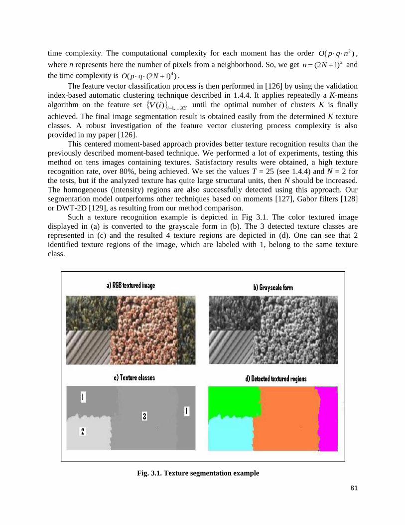
81
time complexity. The computational complexity for each moment has the order )( 2nqpO ,
where n represents here the number of pixels from a neighborhood. So, we get 2)12( Nn and
the time complexity is ))12(( 4 NqpO .
The feature vector classification process is then performed in [126] by using the validation
index-based automatic clustering technique described in 1.4.4. It applies repeatedly a K-means
algorithm on the feature set XYi
iV,...,1
)(
until the optimal number of clusters K is finally
achieved. The final image segmentation result is obtained easily from the determined K texture
classes. A robust investigation of the feature vector clustering process complexity is also
provided in my paper [126].
This centered moment-based approach provides better texture recognition results than the
previously described moment-based technique. We performed a lot of experiments, testing this
method on tens images containing textures. Satisfactory results were obtained, a high texture
recognition rate, over 80%, being achieved. We set the values T = 25 (see 1.4.4) and N = 2 for
the tests, but if the analyzed texture has quite large structural units, then N should be increased.
The homogeneous (intensity) regions are also successfully detected using this approach. Our
segmentation model outperforms other techniques based on moments [127], Gabor filters [128]
or DWT-2D [129], as resulting from our method comparison.
Such a texture recognition example is depicted in Fig 3.1. The color textured image
displayed in (a) is converted to the grayscale form in (b). The 3 detected texture classes are
represented in (c) and the resulted 4 texture regions are depicted in (d). One can see that 2
identified texture regions of the image, which are labeled with 1, belong to the same texture
class.
Fig. 3.1. Texture segmentation example

82
3.1.2. Level set based contour tracking model
The contour-based image segmentation domain has also been widely investigated during
our research. Thus, our PDE–based restoration models described in the second chapter could be
applied successfully in this research field. The nonlinear diffusion-based techniques presented in
1.2 [8] and the variational PDE denoising models described in 1.3 [11] have a strong edge-
preserving character, therefore they can be used for image edge detection. The region boundaries
and these identified edges being closely related, the image segmentation process becomes a quite
easy task.
Other PDE-based segmentation solutions are based on parametric, fast marching [133] and
level-set techniques [123]. We developed a robust level-set based image segmentation approach
that is described in the selected paper 5 published in [134]. Initially introduced by Osher and
Sethian in 1988 to track the moving interfaces [135], the level-set algorithms have since become
a powerful tool for performing contour evolution. The central idea of the level-set based method
is to represent the evolving contour using a signed function whose zero level corresponds to the
actual contour.
The variational level-set techniques perform image object contour tracking by considering
a level set function that minimizes some energy functional. A very popular variational level-set
algorithm is the one elaborated by Chan and Vese [136]. Their algorithm is based on the classical
Mumford-Shah segmentation model [137] and the level sets. It represents a geometric active
contour model that uses variational calculus approaches to evolve the level set function. Our
contour-based PDE segmentation technique is derived from this Chan-Vese level-set model,
representing an improved version of it. Also, in [134] we provide a rigorous mathematical
justification for the proposed level-set based contour detection procedure and for Chan-Vese
model also. We consider the following energy functional:
dxdydxdyHCu
dxdyHCudxdyHdxdyHF
2
3
2
202
2
101
1)(
)(
(3.8)
where yx, is a level-set function defining the contour 0,;, yxyx ,
2R ,
uuuH arctan
1
2
1)( , 0,, i ,
1
001
dxdyHudxdyHuC
and 1
02 11
dxdyHdxdyHuC . The last term is added in order to
regularize the problem and, more precisely, the Euler-Lagrange equations, for giving the
mathematical justification. Then, the functional is rewritten as:
dxdyHCu
dxdyHCudxdyHdxdyF
)1)((
)(
2
3
2
202
2
101
(3.9)

83
Then, we consider in [134] the following minimization problem that has to be solved:
)( ;minarg BVF (3.10)
where )(BV is the space of functions with bounded variations in . In our paper we
demonstrate that there is at least one minimizer for (3.10) (see [134] for more). The Euler-
Lagrange equations corresponding to this minimization problem are then determined as:
0)())()(()(1))()(
)())((22)()())sgn()((
2
022
2
011
'
2022
'
1011
uCuCHCuC
CuCdiv(3.11)
We use the steepest descent method to compute the solution of (3.11) and obtain the
evolution equation:
Tinn
inyxyx
TinFt
,0 ,0
),,(,,0
,0 ,0)(
0
'
(3.12)
Then, (3.12) is solved by the following iterative sequence of equations:
Tinn
in
TinFt
k
k
k
k
,0 ,0
,,0
,0 ,0)(
0
'
(3.13)
where .)(1
0
1 dttT
Tkk
In [134] one proves rigorously that the Cauchy problem
given by (3.13) is well-posed in the space )(BV and the following gradient descent algorithm
is convergent:
)))1((()())1(( ' tktFtktk (3.14)
This level-set based segmentation model is then discretized, and the following numerical
scheme that computes the level-function is obtained:
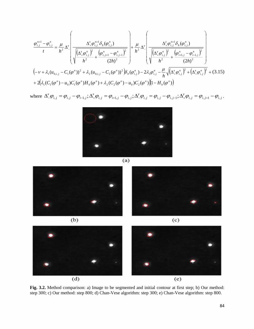
84
)(1)())(()()())((2
2)())(())((
)2(
)(
)2(
)(
'
2022
'
1011
2
,
2
,,3,
2
2,,02
2
1,,01
2
2
,1,1
2
2
,
,
1
,
2
2
2
1,1,
2
2
,
,
1
,
2
,
1
,
n
h
nnn
h
nn
n
ji
xn
ji
xn
ji
n
jih
n
ji
n
ji
n
ji
n
ji
n
ji
y
n
jih
n
ji
y
y
n
ji
n
ji
n
ji
x
n
jih
n
ji
x
x
n
ji
n
ji
HCuCHCuC
hCuCu
hh
h
hh
ht
(3.15)
where jijiji
y
jijiji
y
jijiji
x
jijiji
x
,1,,1,,,,,1,,1,, ;;; .
Fig. 3.2. Method comparison: a) Image to be segmented and initial contour at first step; b) Our method:
step 300; c) Our method: step 800; d) Chan-Vese algorithm: step 300; e) Chan-Vese algorithm: step 800.
85
The obtained iterative algorithm has been tested on various image datasets, being applied
with the following parameters: 1.0,1,1.0,2.0,1321 tt and N = 1000. A
lot of contour tracking experiments have been performed, satisfactory results being achieved. A
high object detection rate, of approximately 90%, is reached, and high values for the
performance parameters are also obtained: Precision = 0.91 and Recall = 0.85. So, the proposed
technique tracks the most relevant objects while identifying more relevant results than irrelevant.
Method comparisons have also been performed. The contour tracking approach described
here provides much better results than other active contour based methods. The performed
experiments prove that our level-set segmentation technique performs better than influential
Chan-Vese contour-based model [136]. Thus, it provides a higher object detection rate and also
executes somewhat faster, identifying the contours in a lower number of iterations. Thus, our
variational approach can be seen as an improved variant of the Chan-Vese model.
A contour tracking example and method comparison is represented in Fig. 3.2. In (a) there
is displayed an image containing human cells that must be segmented. The initial contour is also
depicted in red. The cell segmentation results obtained by our level-set based approach after 300
and 800 iterations are described in (b) and (c). One can see that all the cells are detected. The cell
tracking results produced by the Chan-Vese method are displayed in (d) and (e). The parameters
used for Chan-Vese procedure are 1.0,0,5.0,121 t . The Chan-Vese
algorithm cannot segment all these cells in the same number of steps.
Also, the method described here outperforms also other active contour based techniques
[124,138]. This image segmentation technique using contour tracking has important computer
vision application areas, such as robotics, video object detection and tracking, object
interpretation, biometrics and medical computer vision.
3.2. Temporal video segmentation approaches
While in the previous section we described several segmentation solutions for digital
images, the segmentation of the video sequences is described in this section. We approached in
some of our papers the temporal video segmentation domain [33,139,140]. Temporal video
segmentation has been an area of active research in the last decades. It represents a key step in
video analysis, being successfully applied in various important video analysis domains, such as
video key frame extraction [141], video compression, video indexing [142], video content
browsing and retrieval [143], or video object detection and tracking [144].
This type of video segmentation consists in partitioning the movie in temporal segments,
like shots and scenes. The video shot, sometimes referred as basic scene, represents the
elemental unit of the video clip and refers to a continuous sequence of frames, shot
uninterruptedly by one camera. The video scene represents a succession of several semantically-
correlated shots. Shot transitions are the mechanism used to change from one shot to the next in a
video production. The video shots are assembled during the editing phase using a variety of
technologies that produce different types of shot transitions.
These transition types can be broken basically into three categories: hard cuts, soft cuts
and digital effects. A hard cut, simply referred as cut, represents a sudden transition from one
video shot to another, and is the most common shot transition. A soft cut represents a gradual
transition between two shots, which means a sequence of video frames that belongs to both the
first and the second video shot. There exist two types of soft cuts: fades and dissolves. A fade
comes in two varieties: fade-in and fade-out. A fade-in starts from a solid color screen and
86
slowly transitions to a shot. A fade-out starts with a shot and transitions to a solid color. A
dissolve (cross-fade) occurs when the two video shots overlap for a period of time, the first one
dissolving into the second one. Digital effects for shot transition include wipes, color
replacement, animated effects, pixelization, focus drops, lighting effects, pushes, page peels,
spirals, irises and others.
Obviously, a shot-based video segmentation (video shot detection) process consists of
identifying all the shot transitions within a video sequence. Video cut detection methods can be
grouped in the following categories: pixel-difference based techniques, histogram comparison
based methods, edge-oriented models, motion-based techniques and statistical feature-based
approaches.
In my selected paper 6 [139] a review of all these categories, describing their video shot
identification techniques, is provided. Some histogram-based approaches considered by us are
described in the next subsection. A much more efficient video segmentation technique, which
uses a 2D Gabor filtering based frame feature extraction and an automatic video frame
classification, is described in 3.2.2.
3.2.1. Histogram comparison based shot detection techniques
The most popular video cut detection techniques are those based on different types of
histograms. Intensity and color histogram based methods represent a good alternative to pixel-
based approaches, providing better results.
Numerous distance formulas have been modeled for measuring the similarity of grayscale
(color) histograms corresponding to consecutive frames in a movie. Besides Euclidian metric, we
must mention the histogram differences, the histogram intersection and the histogram quadratic
distance. Also, other types of image histograms, like YUV histograms, weighted histograms
[145] or multiresolution histograms [146] are used as well by the video cut detection algorithms.
A histogram-based video cut detection technique is proposed in my 2006 book [33]. The
grayscale histogram of each video frame is considered as a frame feature vector. The distances
between these feature vectors are computed using Euclidean metric or SAD. Then, two solutions
for frame grouping are provided. The first one represents a semi-automatic approach that sets
interactively the number of videoshots, N, first. Then, the highest N - 1 feature vector distance
values are determined. The values of these locations correspond to the N - 1 video shot
transitions from the analyzed clip. Given the locations of the video cuts, the shot detection
process becomes an easy task.
The other grouping solution is an automatic technique based on local adaptive
thresholding [33]. A video cut is identified whenever the inter-frame difference metric value
exceeds a threshold value. The used threshold is detected automatically, its value depending on
the current pair of consecutive frames.
Both versions of this histogram-based segmentation method were tested on many videos.
They outperform the pixel-difference based techniques using SAD metric, producing much less
false hits and having a higher precision rate. Histogram comparison algorithms provide better
segmentation results than pixel-based approaches because they are not as sensitive to minor
changes within video scenes as pixel based methods. The main drawback of the histogram-based
video cute detection is that the spatial distribution of information is disregarded. Thus, two
images may have quite similar color histograms while their content differs extremely. For
example an image describing a sunflower field beneath a blue sky and an image depicting a sand
87
beach near the sea, could have almost the same histogram. Obviously, a lot of missed hits (video
cuts) may result from this situation.
We tried to overcome this disadvantage of color/intensity histograms, by combining
various histograms into a frame feature vector. So, in [147] we model the video frame feature
vectors as the sum of two normalized histograms. The color, or grayscale histogram, is combined
to the DCT histogram into a more efficient image content descriptor.
The video frame feature vectors, computed as NM
IDCTHIHIV iic
i
))(()()( for
each NM frame iI , are categorized using the semi-automatic grouping approach based on
the number of shots. We obtain better cut detection results using this improved technique, which
are next used for other video analysis processes, like keyframe extraction and video recognition
[147]. More results from this paper [147], related to this computer vision processes, will be
presented in 3.4.2.
I have treated the histogram-based video segmentation algorithms very succinctly in this
short subsection because they do not contain more original contributions. My major contribution
in the temporal video segmentation domain is described in the following, much larger,
subsection.
3.2.2. Automatic feature-based video cut identification model
We developed an automatic feature-based video cut detection technique that is described
in [139]. The most important part of our technique is the feature extraction stage, which produces
some content-based feature vectors that provide an optimal frame characterization. We
considered a two-dimensional Gabor filtering-based feature extraction to obtain some good
frame content descriptors. So, the selected paper [139] considers an even-symmetric 2D Gabor
filter having a quite similar form to that given by (2.31):
)2cos(2
1exp),(
22
,
fxyx
yxGyx
f
, (3.16)
where cossin yxx and sincos yxy . Filter fG , optimally captures both
local orientation and frequency information from a video frame.
Each frame of the analyzed movie is then filtered by applying fG , at various orientations
and a given frequency. A set of proper values for the filter’s parameters, obtained from our
experiments, are used [139]. Thus, we set the following values for frequency and the two
standard deviations: f = 16, 5.4 ,3 yx . Also, we propose the following sequence of six
angle orientations: .;6
5;
3
2;
2;
3;
6654321
As a result, we
obtain the following Gabor filter set: ]6,1[, ifi
G . This even-symmetric 2D Gabor filter set is
described in the next figure, Fig. 3.3, where each filter kernel fiG , is represented as a 3D
surface plot.
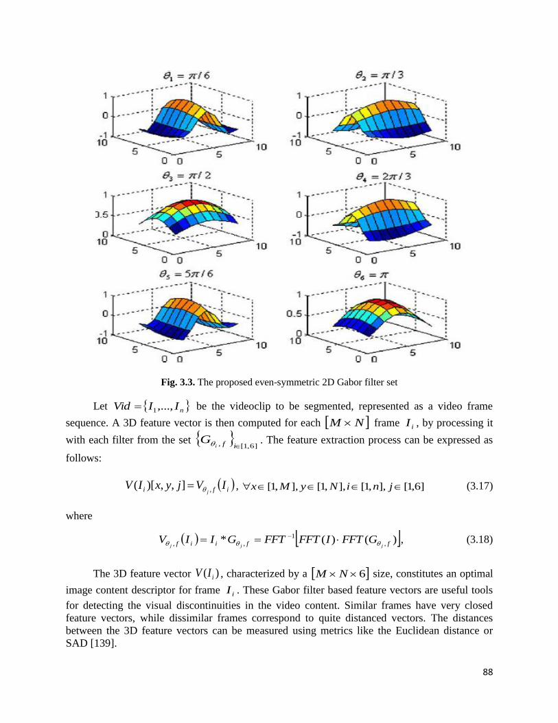
88
Fig. 3.3. The proposed even-symmetric 2D Gabor filter set
Let nIIVid ,...,1 be the videoclip to be segmented, represented as a video frame
sequence. A 3D feature vector is then computed for each NM frame iI , by processing it
with each filter from the set ]6,1[, ifi
G . The feature extraction process can be expressed as
follows:
ifi IVjyxIVj ,],,)[( , ]6,1[],,1[],,1[],,1[ jniNyMx (3.17)
where
)()(* ,
1
,, ffiif jjjGFFTIFFTFFTGIIV , (3.18)
The 3D feature vector )( iIV , characterized by a 6NM size, constitutes an optimal
image content descriptor for frame iI . These Gabor filter based feature vectors are useful tools
for detecting the visual discontinuities in the video content. Similar frames have very closed
feature vectors, while dissimilar frames correspond to quite distanced vectors. The distances
between the 3D feature vectors can be measured using metrics like the Euclidean distance or
SAD [139].
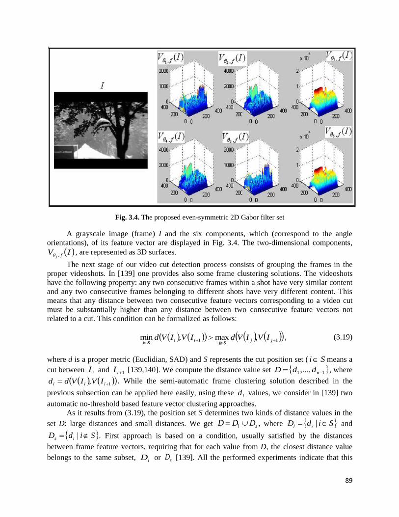
89
Fig. 3.4. The proposed even-symmetric 2D Gabor filter set
A grayscale image (frame) I and the six components, which (correspond to the angle
orientations), of its feature vector are displayed in Fig. 3.4. The two-dimensional components,
IV fj , , are represented as 3D surfaces.
The next stage of our video cut detection process consists of grouping the frames in the
proper videoshots. In [139] one provides also some frame clustering solutions. The videoshots
have the following property: any two consecutive frames within a shot have very similar content
and any two consecutive frames belonging to different shots have very different content. This
means that any distance between two consecutive feature vectors corresponding to a video cut
must be substantially higher than any distance between two consecutive feature vectors not
related to a cut. This condition can be formalized as follows:
11 ,max,min
jjSj
iiSi
IVIVdIVIVd , (3.19)
where d is a proper metric (Euclidian, SAD) and S represents the cut position set ( Si means a
cut between iI and 1iI [139,140]. We compute the distance value set 11,..., nddD , where
1, iii IVIVdd . While the semi-automatic frame clustering solution described in the
previous subsection can be applied here easily, using these id values, we consider in [139] two
automatic no-threshold based feature vector clustering approaches.
As it results from (3.19), the position set S determines two kinds of distance values in the
set D: large distances and small distances. We get sl DDD , where SidD il | and
SidD is | . First approach is based on a condition, usually satisfied by the distances
between frame feature vectors, requiring that for each value from D, the closest distance value
belongs to the same subset, lD or sD [139]. All the performed experiments indicate that this

90
condition is true for our Gabor filter-based feature vectors. So, the values from D are sorted in
ascending order, the largest absolute difference between two consecutive values in the sorted
vector being identified. The lower value is the greatest distance from sD , while the higher one is
the lowest distance from lD , the two distance subsets thus being determined [139].
The other automatic frame clustering solution applies an hierarchical agglomerative
classification procedure using average linkage clustering to the distance set D, until the number
of distance clusters becomes K = 2. The cluster containing the larger values has to be lD , the
distance subset that determines the cut position set S and the video break detection result (see
[139]).
The described temporal video segmentation technique has been tested on hundreds video
sequences. The performed experiments have provided very good segmentation results. A very
high video cut detection rate and high values for the performance parameters have been
achieved. Thus, we have got the following values Precision = 0.94, Recall = 0.96 and F1 =
0.949, respectively.
Method comparison has been also performed. Our automatic feature-based cut detection
technique outperforms the video cut identification methods based on pixel differences, color
(grayscale) histograms, edge histograms, basic statistical features or likelihood ratio. Those
segmentation algorithms produce more false hits and missed hits, therefore providing lower
values for the three quality measures.
Precision, Recall and F1 values obtained from cut detection experiments using the SAD-
based pixel differences, color histograms (CH), edge histograms (EH), simple statistical
measures (dispersion, mean, variance) (ST) and likelihood ratio (LHR) are registered in Table
3.1. One can see in this table that our cut identification algorithm get much higher values for the
performance parameters.
The techniques using pixel difference and those based on histograms execute somewhat
faster than our algorithm, the complex Gabor filtering related computations performed by our
feature extraction approach requiring more processing time [139]. The segmentation models
based on edge histograms or statistical measures are considerably slower than our video cut
identification technique.
Table 3.1. Method comparison: performance measures of various shot detection algorithms
Technique Precision Recall F1
Our method 0.94 0.96 0.949
SAD 0.78 0.76 0.769
CH 0.75 0.70 0.724
EH 0.80 0.74 0.768
ST 0.64 0.61 0.624
LHR 0.60 0.59 0.595

91
In the next figure there is displayed one of our many temporal videoclip segmentation
results [139]. The determined shot cuts of a movie are represented as pairs of frames in Fig. 3.5.
For example, the first two images determine a video break, the third and the fourth indicate
another break and so on. While our technique described here identifies correctly all the 24 shot
cuts of this film, no cuts being missed and no false cuts being detected, the other segmentation
models obtain much weaker results.
Fig. 3.5. Video cuts (as pairs of frames) corresponding of a movie composed of 25 shots.
The positions of the video cuts described in Fig. 3.5 are displayed in Fig. 3.6. As one can
observe in the last figure, there are many differences between the data represented in the graphs
corresponding to the 6 techniques. The highest 24 distance values are marked in each graph on
the first column of the figure. It is obvious that many high distances displayed in the graphs of
SAD, CH, EH, ST and LHR algorithms do not correspond to video cuts. There are 5 such
distance values for SAD, 8 for CH, 3 for EH, 12 for ST and 14 for LHR [139].

92
Fig. 3.6. Method comparison: the video cut detection results of 6 approaches
The method described here has also been tested for other shot transition types. While it
produces optimal cut detection results, our approach performs weaker when applied to gradual
transitions or some digital effects. However, the performed experiments have indicated a
relatively good identification of the starting points of soft transitions like fades and dissolves.
Extending this Gabor filtering based approach in the direction of soft cut detection will constitute
an important task of my future work.

93
3.3. Variational PDE models for image reconstruction
Image reconstruction, known also as image inpainting, represents the computer vision
process of restoring the missing areas of a damaged image as plausibly as possible from the
known zones around them. The image reconstruction techniques are divided into the following
categories: structural inpainting, textural inpainting, and combined approaches that perform
simultaneous structure and texture inpainting.
Texture-based inpainting is highly connected with the problem of texture synthesis. A lot
of texture inpainting algorithms have been proposed since an influential texture synthesis model
was developed by A. Efros and T. Leung [148]. In their approach texture is synthesized in a pixel
by pixel way, by taking existing pixels with similar neighborhoods in a randomized fashion.
Many other texture synthesis algorithms improving the speed and effectiveness of the Efros-
Leung scheme have been elaborated in the last 15 years [149].
Structural inpainting uses PDE-based and variational reconstruction techniques. The PDE
methods follow isophote directions in the image to perform the reconstruction. The first PDE-
based inpainting model was introduced by Bertalmio et al. in [150]. Variational methods for
image reconstruction, which are closely related to the variational denoising models, have been
introduced since 2001, when the Total Variation (TV) inpainting model was proposed by T.
Chan and J. Shen [151]. Their variational scheme fills the missing image regions by minimizing
the total variation, while keeping close to the original image in the known regions. It uses an
Euler-Lagrange equation and anisotropic diffusion based on the strength of the isophotes. The
TV inpainting model has been extended and considerably improved in numerous other papers
[152].
We have proposed a robust variational PDE technique that restores a degraded image that
is observed in a number of points in selected paper 7 [153]. Our approach uses a variational
problem considered in the Sobolev distribution space for which the corresponding Euler-
Lagrange equation is a nonlinear elliptic diffusion equation.
Thus, in [153] the reconstructed image is determined from the following energy
functional minimization:
,)(),(;2
1)),((min 1
0
12
10
HuuLuuudxdyyxug (3.20)
where g: R―> R represents a convex and lower semi-continuous function, u is the restored
image and 0u is the observed image, characterized by missing zones, on bounded domain 2R . The Euler–Lagrange optimality conditions in (3.20) are given by the elliptic boundary
value problem:
on ,0)(
in ,)( 0
u
uuu
(3.21)
where is the subdifferential of g defined as:
RssgrgsrwRwr ),()( ;)( (3.22)

94
and representing a maximal monotone (multivalued) function. In [153] we then demonstrate,
providing a rigorous mathematical proof, that the minimization problem (3.20) has a unique
solution u*, which satisfies the equation given by (3.21). We prove that the steady-state solution
u* to the following evolution equation:
)(0,on ,0
, ),,(),,0(
)(0,in ,)(
0
0
u
yxyxuyxu
uuut
u
(3.23)
represents also the solution to the equation (3.21) and, respectively to the minimization problem
(3.20) (see [153] for more). The discrete version of the equation (3.23) is provided by the
following steepest descent algorithm:
1,... ,)(2 011 kuuuu kkk (3.24)
Then, by using )(uAu , this implicit finite difference scheme is next transformed
into the next explicit finite difference scheme:
NkuuhAu kk
k 0,1,..., ,1 (3.25)
where N is the number of iterations, Tt ,0 and Nh = T. By replacing A to the discretized
second order operator, k
ji
k
ji
k
ji
k
ji
k
ji uuuuuAu ,1,1,,1,1 44
1 , where ),(, jiuu kk
ji , one
obtains:
)(4)()()()(4
,1,1,,1,1,
1
,
k
ji
k
ji
k
ji
k
ji
k
ji
k
ji
k
ji uuuuuh
uu
(3.26)
If 1 rr , instead of (3.26) we consider the following explicit finite difference
scheme:
k
ji
k
ji
k
ji
k
ji
k
ji
k
ji
k
ji
k
ji uuuuuuuu ,1,1,,1,1,,
1
, 4
(3.27)
where 1 and 1 ,0 respectively.
The image is reconstructed by applying the iterative algorithm given by (3.27) for
k=0,1,…, N – 1. The degraded image 0
0 uu is transformed into the restored image Nu , that is
closed to the original image, in several tens steps [153].
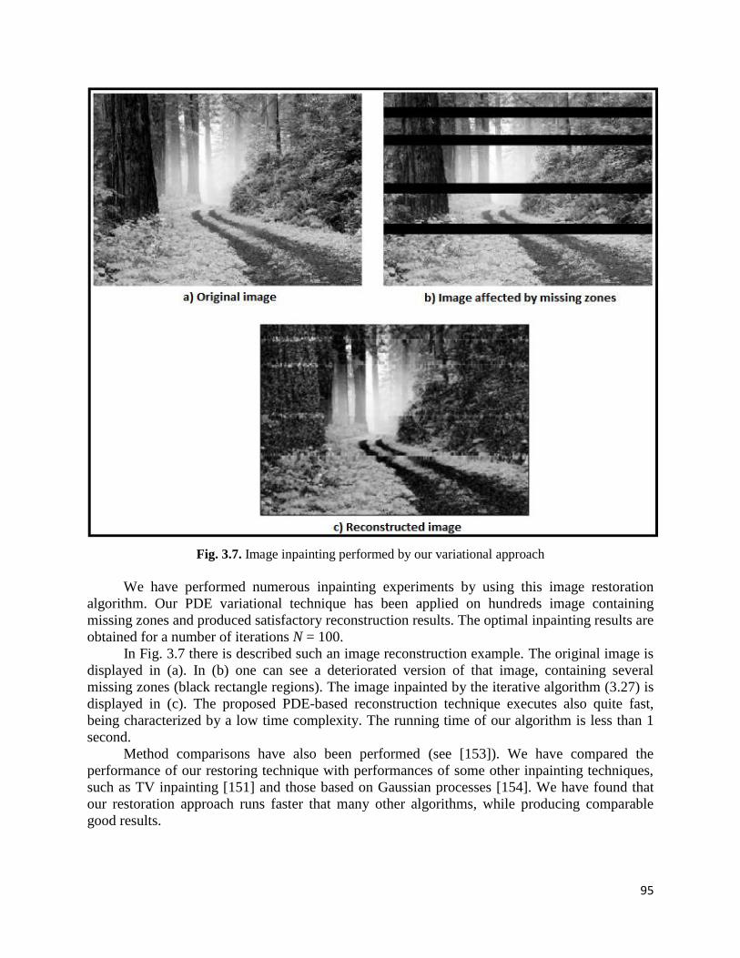
95
Fig. 3.7. Image inpainting performed by our variational approach
We have performed numerous inpainting experiments by using this image restoration
algorithm. Our PDE variational technique has been applied on hundreds image containing
missing zones and produced satisfactory reconstruction results. The optimal inpainting results are
obtained for a number of iterations N = 100.
In Fig. 3.7 there is described such an image reconstruction example. The original image is
displayed in (a). In (b) one can see a deteriorated version of that image, containing several
missing zones (black rectangle regions). The image inpainted by the iterative algorithm (3.27) is
displayed in (c). The proposed PDE-based reconstruction technique executes also quite fast,
being characterized by a low time complexity. The running time of our algorithm is less than 1
second.
Method comparisons have also been performed (see [153]). We have compared the
performance of our restoring technique with performances of some other inpainting techniques,
such as TV inpainting [151] and those based on Gaussian processes [154]. We have found that
our restoration approach runs faster that many other algorithms, while producing comparable
good results.
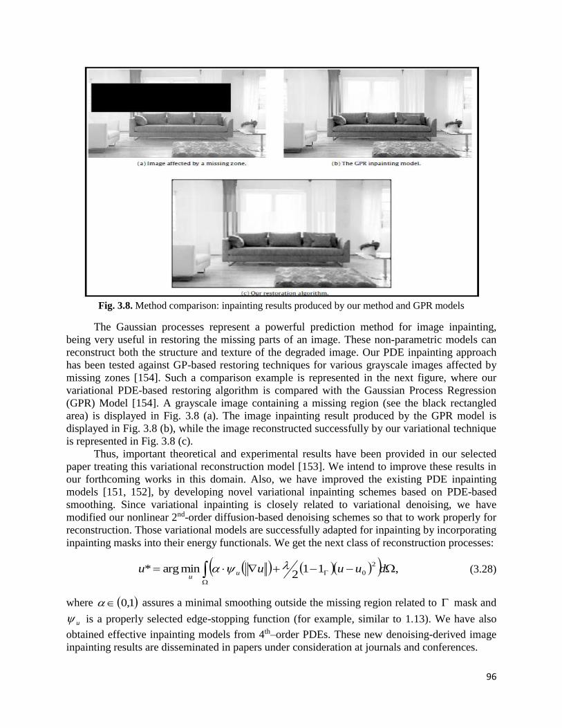
96
Fig. 3.8. Method comparison: inpainting results produced by our method and GPR models
The Gaussian processes represent a powerful prediction method for image inpainting,
being very useful in restoring the missing parts of an image. These non-parametric models can
reconstruct both the structure and texture of the degraded image. Our PDE inpainting approach
has been tested against GP-based restoring techniques for various grayscale images affected by
missing zones [154]. Such a comparison example is represented in the next figure, where our
variational PDE-based restoring algorithm is compared with the Gaussian Process Regression
(GPR) Model [154]. A grayscale image containing a missing region (see the black rectangled
area) is displayed in Fig. 3.8 (a). The image inpainting result produced by the GPR model is
displayed in Fig. 3.8 (b), while the image reconstructed successfully by our variational technique
is represented in Fig. 3.8 (c).
Thus, important theoretical and experimental results have been provided in our selected
paper treating this variational reconstruction model [153]. We intend to improve these results in
our forthcoming works in this domain. Also, we have improved the existing PDE inpainting
models [151, 152], by developing novel variational inpainting schemes based on PDE-based
smoothing. Since variational inpainting is closely related to variational denoising, we have
modified our nonlinear 2nd-order diffusion-based denoising schemes so that to work properly for
reconstruction. Those variational models are successfully adapted for inpainting by incorporating
inpainting masks into their energy functionals. We get the next class of reconstruction processes:
,112
minarg*2
0
duuuu uu
(3.28)
where 1,0 assures a minimal smoothing outside the missing region related to mask and
u is a properly selected edge-stopping function (for example, similar to 1.13). We have also
obtained effective inpainting models from 4th–order PDEs. These new denoising-derived image
inpainting results are disseminated in papers under consideration at journals and conferences.
97
3.4. Image and video recognition methods
Media pattern recognition represents an important computer vision domain, which have
been widely investigated during our research activity. In this section we describe our results
obtained in the pattern recognition subdomains related to image and video data. Image and video
recognition field is strongly correlated to other computer vision domains approached by us and
described in the next sections, such as: image and video retrieval, image object detection and
video object tracking.
The recognition of any media entity represents the process of classification of that entity
on the basis of its extracted features. Depending on the character of the classification approach,
the recognition process can be either supervised or unsupervised. Image and video recognition
area include recognition techniques for images, videos, image objects and video objects. A lot of
such recognition methods were proposed in my past papers. I present some of these approaches
in the following subsections. Several automatic image recognition techniques are described in
the next subsection. Then, in 3.4.2, a video sequence recognition approach is presented. Next,
some image and video object recognition models are discussed in the last subsection.
3.4.1. Automatic image recognition techniques
We considered the task of automatic recognition of entire images in some of our past
papers [33,155-159], developing both supervised and unsupervised recognition methods. The
automatic classification algorithms used for image recognition are those described in 1.4, so we
focus on image feature extraction instead. The existing image featuring approaches use various
histograms [160,161], Gabor filtering [77], 2D Wavelets [162], SIFT characteristics [84] and
others. We have provided better feature extraction solutions during our research in this field.
A supervised image recognition system classifies any input image using a training image
set. A feature extraction process is performed on the (input) images to be classified and the
registered images from the training set. Then, any input feature vector is compared to the vectors
from the training feature set. The most supervised image recognition techniques developed by us
are related to biometrics [53]. In the sections 1.2 and 1.3 of the second chapter we have treated
the recognition of images representing biometric identifiers such as faces and fingerprints. The
numerous biometric authentication systems described there, using PCA [75], Gabor [79,80,97],
or Wavelet [97-99] features, and performing identification and verification of faces and
fingerprints, represent examples of efficient supervised image recognition systems.
An unsupervised image recognition procedure performs a clustering within a set of
images, on the basis of their content similarity. It uses no training set and if it has also an
automatic character, no knowledge about clusters’ number is available. We have proposed
several automatic unsupervised image recognition approaches, using various feature extraction
and classification algorithms [33,37,155-159]. Each image is featured by computing a proper
content descriptor for it that is used as a feature vector. Then, all feature vectors are clustered
automatically by using the unsupervised classification techniques described in 1.4.
Thus, in [157] we propose an automatic image recognition method using dispersion-based
features. The task to be solved is formulated for all recognition techniques as following: given a
large image set },...,{ 1 nIIS , its images have to be categorized in some classes, whose number
is not a priori known.

98
A grayscale conversion is operated on these images first. Then, each image iI is
decomposed into [a x b] blocks, usually considering a = b. If a perfect division is not possible,
the image could be padded with zeros. The statistical dispersion (standard deviation) of each
block is then computed as the square root of its variance, a dispersion matrix thus being obtained
for each image [155,157]. This matrix is utilized as the image feature vector )( iIV .
The 2D feature vector classification is performed using the region-growing based
automatic clustering algorithm from 1.4.3 [39]. The obtained classes represent a reliable image
recognition result, each class containing similar regions while non-similar images belong to
different clusters [157]. The performed numerical experiments produced good recognition results
and a quite high recognition rate. Although this approach works properly for large image sets, we
provide here, as an example, a recognition process applied to a small image set. The color
images to be clustered are displayed in Fig. 3.9. The 2D feature vectors are represented as 3D
plots in Fig. 3.10, the distances between them being registered in Table 3.2. The clustering
process using the values of this table provides the image recognition result: 531 III , 42 II .
Fig. 3.9. The color image set
Fig. 3.10. The feature vector set
1 2 3
4 5
0
50
0
20
400
50
100
1
0
50
0
20
400
50
100
2
0
50
0
20
400
50
100
3
0
50
0
20
400
50
100
4
0
50
0
20
400
50
100
5

99
Table 3.2. Distances between image feature vectors
)( 1IV )( 2IV )( 3IV )( 4IV )( 5IV
)( 1IV 0 571.3183 293.0381 675.6527 319.3169
)( 2IV 571.3183 0 599.5098 359.3718 618.9163
)( 3IV 293.0381 599.5098 0 686.5573 361.6215
)( 4IV 675.6527 359.3718 686.5573 0 712.8829
)( 5IV 319.3169 618.9163 361.6215 712.8829 0
We also developed some moment-based image recognition approaches [156,158,159]. The
area moments represent not only good texture descriptors but also very good content descriptors,
given the fact that image content is composed of textures, colors and shapes.
Thus, in [158] we propose an automatic moment-based image recognition technique. A
moment-based image analysis similar to that described in subsection 3.1.1 is performed to each
image iI . Its feature vector is modeled as a sequence of 12 moment-based coefficients,
representing normalized centered discrete area moments:
),,,,,,,,,,,()( 232221201312111003020100 iIV (3.29)
where
)(
)(ˆ )(
00 i
ipq
ipqI
II
(3.30)
where 12
qp
, the improved centered moment of (p+q)th order pq̂ is given by (3.4) and
the centered moment of (p+q)th order pq is computed as in (3.7).
The computed feature vector provides a robust image content description [158]. Next, an
automatic feature vector clustering is performed within the feature set )}(),...,({ 1 nIVIV . The
automatic unsupervised classification algorithm presented in 1.4.4, here using a hierarchical
agglomerative procedure with average linkage clustering and a validity index-based measure, is
successfully applied in this case. Euclidian metric is used for measuring the distances between
feature vectors. Automatic clustering makes this method work properly for very large image sets.
We have conducted a lot of recognition experiments, testing the proposed technique on
hundreds large image data sets, and achieved quite satisfactory image recognition results. A high
recognition rate, of approximately 80%, has been also obtained [158,159]. Let us describe a
small recognition example performed by using this moment-based approach.
100
Fig. 3.11. Images to be clustered
The distances between feature vectors of the images to be recognized, displayed in Fig. 3.11, are:
))(),(( 21 IVIVd 7.14, ))(),(( 31 IVIVd 2.26, ))(),(( 41 IVIVd =6.45, ))(),(( 51 IVIVd 2.77, ))(),(( 32 IVIVd
7.91, ))(),(( 42 IVIVd =7.51, ))(),(( 52 IVIVd =7, ))(),(( 43 IVIVd =7.17, ))(),(( 53 IVIVd =2.14, ))(),(( 54 IVIVd
= 6.29. The image clusters obtained on the basis of these values are },,{ 531 III and },{ 42 II .
Another automatic moment-based image recognition technique developed by us is provided in
[156]. The feature vectors are modeled as sequences of normalized centered area moments, but having
different forms than sequences given by (3.29). In the classification stage it uses the automatic feature
vector clustering algorithm from 1.4.3 [39] and provides very good image categorization results [156].
Other image feature vector models, such as those based on various types of histograms, are
provided by us in [147]. Image color/intensity histogram does not represent a satisfactory content
descriptor, for the reasons explained in 4.2.1, so it has to be combined to other image histograms, such
as DCT histogram, to obtain better content descriptors [147]. Also, the 2D Gabor filtering-based 3D
feature vectors modeled for the video shot detection process described in 3.2.2 can be successfully used
for unsupervised content-based image recognition, because they represent robust image content
descriptors [139]. In section 3.5 we will describe some efficient feature vectors based on Gabor filters,
which are used for content-based image retrieval [163].
Image clustering can also be performed by using various image similarity metrics [164]. In [164]
we develop a robust image similarity metric based on SIFT characteristics. The proposed content
similarity metric could be used successfully for performing efficient automatic image recognition.
Another category of image recognition techniques constructed by us is that of color-based
recognition approaches [165]. We have developed several automatic image recognition methods using
LAB color features in the last four years [165-167]. We have replaced RGB color space with LAB in our
image analysis because the characteristics of the LAB color space makes it more suitable for extracting
global color features from a digital image.
Thus, a robust unsupervised color-based image recognition system is proposed in [165]. The
images from a given set },...,{ 1 nIIS are clustered in several categories on the color similarity basis.
First, all these images are converted from RGB to LAB. A certain color is defined in LAB space by a
triplet (L,a,b), where (a,b) can be viewed as a pure color, while L coordinate gives its darkness or
lightness. A reduction of the number of colors is required in order to obtain global characteristics [166].
With the LAB color space, such a reduction can be done by considering only several ab planes from the

101
total of 256. We use 8 ab planes corresponding to the following central L values: 16, 48, 80, 112, 144,
176, 208 and 240. Any value of L in an image is forced to take the nearest value from this set. Then, for
each of the 8 ab planes, we construct one planar histogram, having [256 x 256] bins, one for each (a,b)
pair. We clear the bins containing less than 20 points, the planar histogram becoming scarce in values
(with many empty bins). So, we compute one important color for several subsets of possible colors. The
colors in a ab plane are distributed as in Fig. 3.12: red colors in upper right quadrant, and here, at the
border of upper left quadrant, yellow color at higher luminance values; violet nuances in the lower right
quadrant, blue colors in lower left quadrant and green colors in upper left quadrant. Black and white
appear in planes with the lowest and highest luminance, and gray tones appear mostly toward center of
ab planes.
Fig. 3.12. Color distribution for L=134 ab plane
So, we consider each quadrant of an ab plane as an independent subset of colors. As we
take into consideration 8 ab planes, we have 32 quadrants where we must identify the most
important colors. For each quadrant a list of (a,b) pairs with corresponding nonzero bins in the
planar histogram is constructed. Then the (a,b) pairs are ordered according to the values in the
bins, the colors with a greater number of corresponding pixels in the image being on top of this
list. Then colors very close in the ab planes are merged in these lists, which became a list of
fewer colors, but with larger counts of pixels. Finally, the top (a,b) pair is taken as the most
important color in the corresponding quadrant. Collecting all the 32 important colors provides us
the following 2D feature vector:
i
i
i
j
i
j
i
i
ib
a
b
a
b
aIV
32
32
1
1)(
(3.30)
each column representing an important ),( ii ba color. In order to facilitate the image comparison
process, the feature vector components are arranged in order, from lower luminance ab planes to
higher luminance, and clockwise from upper right quadrant to upper left quadrant. This assures
that comparing two similar color components of two images means comparing the distance
between two points in the same ab plane and the same quadrant [165].
Euclidean metric is used for these 2D feature vectors in the classification process. These
102
color-based feature vectors are clustered automatically by applying the validation index based
unsupervised classification model described in subsection 1.4.4. In this case that clustering
technique uses the K-means algorithm as the semi-automatic clustering procedure to be executed
repeatedly [165].
We have obtained satisfactory image clustering results, as resulting from our recognition
experiments. Such a color-based image recognition example is represented in Fig. 3.13. The 9
color images are categorized successfully in 4 classes, representing flowers, horses, vestiges and
beaches, on the color similarity basis. A high image recognition rate (over 80%) and high values
for Precision and Recall performance parameters have been also achieved.
Fig. 3.13. Images clustered in 4 color-based classes
Another successfully variant of this LAB color space based recognition approach is
proposed in [166]. A quite similar feature extraction process is performed, but the LAB color-
based image feature vectors are classified by using the hierarchical agglomerative clustering
solution, instead of K-means, within the automatic clustering technique from 1.4.4. Another
efficient LAB color feature based method developed by us is described in [167]. These LAB
color characteristics are also used by us in the biometric domain, for iris clustering [54]. A color-
based iris image recognition system is proposed in [54]. From the performed method comparison
we have found that our color-based recognition methods outperforms other color image
clustering approaches, such as those based on color histograms or some similarity metrics.
We have described here some robust automatic image recognition approaches using
statistics-based, moment-based, Gabor filtering-based, SIFT-based and LAB color-based feature
extraction processes. They provide good results and high recognition rates, outperforming some
state-of-the-art image recognition techniques. Also, because of their automatic character, our
unsupervised recognition methods work properly for very large image sets or databases. For this
reason they can be applied successfully in content-based image indexing and retrieval areas. So,
cluster-based image indexing as well as content-based image retrieval (CBIR) can be easily
performed using the image recognition results described here, as we will see in the next section.

103
3.4.2. Video sequence recognition approach
Besides static image recognition, we have considered developing some video image
recognition solutions. An unsupervised content-based movie recognition technique is provided in
[147]. Our approach clusters successfully the video sequences on the basis of their content-
similarity.
So, in [147] we consider a set of videos, },...,{ 1 NVidVid , that must be classified in several
similarity clusters. Each video sequence iVid could be composed of one or more video shots
[147]. The proposed video analysis algorithm consists of the following processes:
Video frame feature extraction
Temporal video segmentation
Video keyframe extraction
Movie feature vector modeling
Video feature vector clustering
In the frame feature extraction stage one computes powerful frame content descriptors that
can be used as feature vectors in the next video analysis processes. Feature extraction could be
performed using the numerous image featuring techniques described in this thesis. In our 2005
paper [147] we considered a histogram-based frame feature extraction, but since then we have
provided much more efficient featuring approaches [155-157,163-166]. We already mentioned in
3.2.1 the feature extraction process from [147], which computes a normalized combination of
color (intensity) histograms and DCT (Discrete Cosinus Transform) histograms. The feature
vectors are obtained as NM
IDCTHIHIV iic
i
))(()()( for each NM frame iI [147].
A temporal video segmentation process is then performed on each videoclip iVid , to
determine its shots. In [147] a semi-automatic video cut detection approach, like those described
in 3.2.1, is used. Obviously, our automatic videoshot detection technique developed in 2009 and
presented in 3.2.2 [139] would represent a better segmentation solution in this case.
The analyzed clips may have a large size, which means a great number of frames,
therefore some resumed forms of the videos are used in the recognition process. A resumed form
of the movie iVid is determined by computing its keyframes [147]. The video keyframes
comprise the essence of the movie content. The easiest video keyframe detection solution
consists of considering the first frame of each identified videoshot as a keyframe, but this does
not represent always a proper solution.
We could extract more keyframes from each shot by performing a frame clustering
operation within that shot. In [147] we use a semi-automatic hierarchical agglomerative
clustering procedure for frame grouping, the number of clusters being set interactively after
watching the videoshot. This region-growing algorithm could be replaced with one of the
automatic clustering techniques described in 1.4. The first video frame of each cluster is
considered a keyframe of the videoshot [147]. The keyframe set of the movie sequence includes
all keyframes of all the videoshots.
A video feature vector is then modeled for each movie. Therefore, if },...,{ )(1
i
in
i II
represents the keyframe set of iVid , then the movie feature extraction process is expressed as
[147]:

104
Ni
IV
IV
VidVi
in
i
i ,1,
)(
...
)(
)(
1
(3.31)
Each 2D video feature vector iVidV is a 256)( in matrix that represents a good
content descriptor of the corresponding movie. So, all these feature vectors are characterized by
the same number of columns and a number of rows depending on the number of keyframes from
each video. Therefore, the distances between them cannot be measured by using Euclidian metric
or other conventional metrics. In this case, which requires a special metric to be used in the
classification process, the Hausdorff-derived metric, described in 1.4.1 and used also for speaker
recognition tasks, can be successfully used.
An unsupervised videoclip classification is then performed by clustering these 2D feature
vectors. In [147] a semi-automatic feature vector clustering procedure, based on a hierarchical
agglomerative algorithm, is applied to the feature set NiiVidV
,1. The number of the video
classes, K, is set interactively after one visualizes these videos [147]. Obviously, an automatic
clustering algorithm [39], like those presented in 1.4, can be used in this case, instead of the
semi-automatic region-growing approach, too.
We have tested the proposed recognition approach on numerous video sets, obtaining quite
good results. This main disadvantage of this unsupervised video recognition technique consists
of its non-automatic character. Because of the interactivity that is used in several stages of the
recognition process, our approach executes quite slowly. Also, because of the same interactions,
it is quite difficult to perform clustering within very large movie sets. For small and medium sets
of videos, this recognition approach works properly, as resulting from the following example,
too. We consider the small video set 321 ,, VidVidVid , to be clustered. The keyframes of these
videos and the keyframe feature vectors are displayed in the next three figures. The values of
distances between movie feature vectors V( 31Vid ) are included in Table 3.3. By using the
values in this tables, the videos are clustered in 2 classes: 31,VidVid and 2Vid .
Fig. 3.14. Keyframes of the 1st movie and their feature vectors
105
Fig. 3.15. Keyframes of the 2nd movie and their feature vectors
Fig. 3.16. Keyframes of the 3rd movie and their feature vectors
Table 3.3. Distances between video feature vectors
)( 1VidV )( 2VidV )( 3VidV
)( 1VidV 0 0.1168 0.0191
)( 2VidV 0.1168 0 0.1147
)( 3VidV 0.0191 0.1147 0
This video recognition method can be improved considerably by transforming it into an
automatic approach. We have already indicated where our automatic clustering algorithms can
replace the used semi-automatic clustering procedures, so that the recognition technique becomes
completely automatic. An automatic version of this approach can be applied successfully in the
video indexing, where it may provide cluster-based indexing solutions, and retrieval domains.
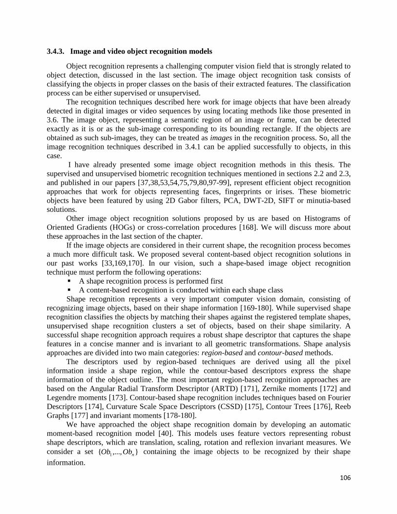
106
3.4.3. Image and video object recognition models
Object recognition represents a challenging computer vision field that is strongly related to
object detection, discussed in the last section. The image object recognition task consists of
classifying the objects in proper classes on the basis of their extracted features. The classification
process can be either supervised or unsupervised.
The recognition techniques described here work for image objects that have been already
detected in digital images or video sequences by using locating methods like those presented in
3.6. The image object, representing a semantic region of an image or frame, can be detected
exactly as it is or as the sub-image corresponding to its bounding rectangle. If the objects are
obtained as such sub-images, they can be treated as images in the recognition process. So, all the
image recognition techniques described in 3.4.1 can be applied successfully to objects, in this
case.
I have already presented some image object recognition methods in this thesis. The
supervised and unsupervised biometric recognition techniques mentioned in sections 2.2 and 2.3,
and published in our papers [37,38,53,54,75,79,80,97-99], represent efficient object recognition
approaches that work for objects representing faces, fingerprints or irises. These biometric
objects have been featured by using 2D Gabor filters, PCA, DWT-2D, SIFT or minutia-based
solutions.
Other image object recognition solutions proposed by us are based on Histograms of
Oriented Gradients (HOGs) or cross-correlation procedures [168]. We will discuss more about
these approaches in the last section of the chapter.
If the image objects are considered in their current shape, the recognition process becomes
a much more difficult task. We proposed several content-based object recognition solutions in
our past works [33,169,170]. In our vision, such a shape-based image object recognition
technique must perform the following operations:
A shape recognition process is performed first
A content-based recognition is conducted within each shape class
Shape recognition represents a very important computer vision domain, consisting of
recognizing image objects, based on their shape information [169-180]. While supervised shape
recognition classifies the objects by matching their shapes against the registered template shapes,
unsupervised shape recognition clusters a set of objects, based on their shape similarity. A
successful shape recognition approach requires a robust shape descriptor that captures the shape
features in a concise manner and is invariant to all geometric transformations. Shape analysis
approaches are divided into two main categories: region-based and contour-based methods.
The descriptors used by region-based techniques are derived using all the pixel
information inside a shape region, while the contour-based descriptors express the shape
information of the object outline. The most important region-based recognition approaches are
based on the Angular Radial Transform Descriptor (ARTD) [171], Zernike moments [172] and
Legendre moments [173]. Contour-based shape recognition includes techniques based on Fourier
Descriptors [174], Curvature Scale Space Descriptors (CSSD) [175], Contour Trees [176], Reeb
Graphs [177] and invariant moments [178-180].
We have approached the object shape recognition domain by developing an automatic
moment-based recognition model [40]. This models uses feature vectors representing robust
shape descriptors, which are translation, scaling, rotation and reflexion invariant measures. We
consider a set },...,{ 1 nObOb containing the image objects to be recognized by their shape
information.
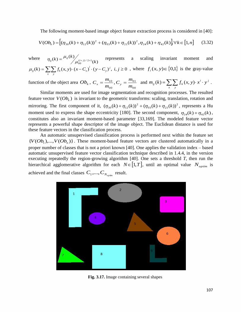
107
The following moment-based image object feature extraction process is considered in [40]:
nkkkkkkkObV k ,1,)()(,))()(())()(()( 4224
2
2103
2
1230
(3.32)
where )(
)()( 12/)(
00 k
kk ji
ijij
represents a scaling invariant moment and
0, ,)()(),()( jiCyCxyxfk j
y
i
x y
xkij , where 1,0),( yxf i is the gray-value
function of the object area kOb , 00
01
00
10 ,m
mC
m
mC yx
and
x y
ji
kij yxyxfkm ),()( .
Similar moments are used for image segmentation and recognition processes. The resulted
feature vector )( kObV is invariant to the geometric transforms: scaling, translation, rotation and
mirroring. The first component of it, 2
2103
2
1230 ))()(())()(( kkkk , represents a Hu
moment used to express the shape eccentricity [180]. The second component, )()( 4224 kk ,
constitutes also an invariant moment-based parameter [33,169]. The modeled feature vector
represents a powerful shape descriptor of the image object. The Euclidean distance is used for
these feature vectors in the classification process.
An automatic unsupervised classification process is performed next within the feature set
)}(),...,({ 1 nObVObV . These moment-based feature vectors are clustered automatically in a
proper number of classes that is not a priori known [40]. One applies the validation index – based
automatic unsupervised feature vector classification technique described in 1.4.4, in the version
executing repeatedly the region-growing algorithm [40]. One sets a threshold T, then run the
hierarchical agglomerative algorithm for each TN ,1 , until an optimal value optimN is
achieved and the final classes optimNCC ,...,1 result.
Fig. 3.17. Image containing several shapes
108
Many experiments have been performed using the described shape recognition approach,
very good results being obtained. A high recognition rate, of approximately 85 %, is produced by
our technique. This recognition rate rises if one increases the threshold value, usually set as
2/nT , but the procedure complexity and time execution rise too.
We obtain high values for the performance parameters (Precision, Recall and F1) of this
recognition process. Thus, we get Precision = 0.85, Recall = 0.84, which means our shape
recognition approach produces quite few missed hits or false positives. A shape recognition
example is described in the two figures. Thus, in Fig. 3.17 there is displayed an image containing
objects which can be segmented easily. Each iOb is marked with the i value in the picture, i =
1,…,9. The shape classes corresponding to the image from Fig. 3.17 are represented in Fig. 3.18,
where each shape is labeled with its class number. The 4 detected shape classes, representing the
final recognition result, are: },{ 91 ObOb , },,{ 642 ObObOb , },{ 83 ObOb and },{ 75 ObOb .
Fig. 3.18. The detected shape-based classes
Our moment-based shape analysis approach outperforms other recognition techniques, like
those based on Hu moments [180], Zernike moments [172] or Fourier descriptors [174]. Also, its
automatic character makes it better than any non-automatic shape recognition approach, because
it works properly for very large sets of shapes. Therefore, it becomes very useful in some
important computer vision application areas, such as shape-based indexing of image databases
and object retrieval from these databases.
In the next stage of object recognition, a content-based recognition is performed within
each shape-based class, iC , Ni ,1 . All the image objects from such a class have similar
shapes but could have different contents. Besides its shape, the object content is characterized by
the colors and textures. Various featuring techniques can be used to obtain a proper image object
content descriptor. A histogram-based feature extraction can be used, the feature vector of an
object from a shape class being computed as a given type of histogram of that object or as a
combinations of more histograms. Color, or intensity, histograms, DCT histograms, edge
109
histograms, weighted histograms or combinations of these image histograms can be used for this
purpose. Such a histogram-based object featuring is proposed by us in our 2006 book [33]. We
have obtained quite good recognition results using these histogram-based feature vectors, but,
since 2006, more powerful image feature vectors that can be applied successfully for image
objects have been modeled by us. So, the feature vectors based on 2D Gabor filters [139], 2D
Discrete Wavelets [99], SIFT characteristics [39,164], statistical features [157] and LAB color-
based characteristics [165-167] can be easily adapted in order to work for image objects.
The content-based feature vectors are clustered automatically using any of the clustering
approaches from 1.4. As a result of this content-based object recognition, each shape class iC is
divided into several content-based sub-classes. All these content classes could be considered the
final object recognition result, although in [33] we consider one more recognition level. Thus, a
structure-based object recognition is performed within each content-based class [33]. The object
structure is defined there as formal model that defines the way color/intensity and texture regions
are arranged into that object. Some structure-based object feature vectors are computed and
clustered in a number of classes [33]. These structure-based classes, containing objects
characterized by the same shape, content and structure, represent the final object recognition
result [33].
The image object recognition approach based on shape, content and structure features
represents a quite good idea, given the satisfactory recognition results it produces [33]. But the
structure-based recognition level has been mainly necessary because of the histogram-based
feature vectors used in [33,169], which do not represent very powerful object content descriptors.
For example, two objects may have exactly the same shape and similar color histograms, but
they could have somewhat different contents because of the different structures (different
arrangements of color regions). We have found that the more complex and robust image feature
vectors constructed by us since 2006, representing much better content descriptors, make the
structure-based recognition process unnecessary, the object recognition being performed
successfully in two stages only.
The recognition methods discussed here can be applied also for video image objects. If the
video objects are defined as image objects contained by video frames, the video object
recognition process becomes equivalent to the video tracking process that is described in the last
section. But if we consider the video object as an entity composed from all its instances in the
frames and its trajectory, the recognition process becomes a more difficult task. In [33] we
consider a recognition solution for such spatio-temporal video objects. Two objects are similar if
they have both similar states and similar trajectories. Similarity measures between object
trajectories are modeled in [33].
These image object recognition methods can be successfully applied not only in image
indexing and retrieval, and video tracking domains, but also in a high-level image analysis and
computer vision field that is image and video interpretation [33]. In [33] we perform also
semantic object analysis, providing some image and video interpretation (understanding)
approaches. A supervised object recognition system is used for this purpose. Its training set
contains registered objects, labeled with their semantic (for example people, car, building, …). A
object feature extraction is performed, then a supervised classification is applied to the feature
vectors [33]. Each input object is inserted in a class representing a semantic (label) by using the
minimum average distance or the K-Nearest Neighbors classifier. The classified (recognized)
object receives the label of that class. An image is interpreted by associating to it the sequence of
labels of its objects. The interpretation of a video results from its frame interpretations [33].

110
3.5. Content-based image indexing and retrieval systems
Multimedia information indexing and retrieval represents an important computer vision
domain that includes two strongly correlated sub-domains. Information indexing is generally
considered an essential requirement for any efficient information retrieval system. The indexing
process develops some structures, called indexes, which facilitate the direct access to required
information from a large data collection. Information retrieval represents the process of
extracting the relevant information to an information need from data collections, eventually
using the index structures.
Multimedia retrieval aims to extract relevant media entities, such as sounds, images,
videos or image/video objects, from multimedia data collections, such as the multimedia
databases [181]. Multimedia indexing and retrieval processes may have a concept-based
character or a content-based character. The concept-based indexing/retrieval is based on
metadata, which refers to the textual descriptions or annotations associated to the media entities.
The content-based indexing/retrieval use the content characteristics, expressed as feature vectors,
of those entities and not their metadata. In [33] we investigated this computer vision domain,
providing some solutions for multimedia database organizing, indexing and retrieval.
Content-based image indexing and retrieval represents the most important and researched
sub-domain of multimedia indexing and retrieval. Some image indexing techniques are described
in the next subsection, while content-based image retrieval approaches are presented in
subsection 3.5.2.
3.5.1. Content-based image indexing models
The content-based image indexing (CBII) has been introduced to overcome the
disadvantages of metadata-based indexing. Content-based image indexing replaces the search
keys, used by annotation-based indexing, with feature vectors characterizing the image content
given by colors/intensities, textures and shapes. An efficient content-based image storing is also
necessary for a flexible retrieval from image databases. The purpose of storing an image
indexing structure is to optimize speed and performance in identifying relevant digital images for
a search query.
A lot of indexing techniques have been developed in the last three decades for the
multidimensional spaces like the content-based image feature vector spaces. Spatial Access
Methods (SAM) based on various tree structures are used for indexing high-dimension spatial
data. Some well-known tree-based indexing methods that work properly for digital images are
the R*-tree [182], K-D-tree [183], VP (Vantage-Point)-tree [184], M-tree and MVP-tree [185].
These content-based indexing solutions treat the image retrieval tasks as multidimensional
Nearest-Neighbor (NN) searches.
The content-based image and object feature vectors modeled by us and described in
previous sections can be successfully used with these SAM-based indexing structures in the
retrieval processes [181]. So, in [186] we have developed a color-based image indexing method
using LAB color features and a K-D tree structure, which recursively partition the space into two
subspaces. Each non-leaf node of the K-D tree generates a splitting plane dividing the space into
two half-spaces. The color-based feature vectors )( iIV , which will be described in 3.5.2, are
inserted in the nodes of this K-D tree as following: the tree is traversed starting from its root and

111
moving to either the left or the right child-node depending on whether the point to be inserted is
on the left or right side of the splitting plane. Once one reaches the node under which the child-
node must be located, insert the new point, representing a feature vector, as either the left or right
child of the leaf node, again depending on which side of node's splitting plane contains the new
node. This K-D tree based index facilitates considerably the image retrieval process, by solving
the K-NN Search task [186]. The image feature extraction and the content-based retrieval using
the K-D-tree based index are described in 3.5.2 [186].
We also consider some cluster-based indexing approaches in [33]. Since the image content
is composed of textures, colors/intensities and shapes, the content-based image indexing include
color-based indexing, texture-based indexing and shape-based indexing procedures [33]. So, an
index is constructed for each content component (color, texture or shape).
The idea of our image indexing approach is to model a content-based image database
recording and to perform a clustering process at the level of each field of that recording [33]. So,
let NII ,...,1 be the images from a large collection. A robust image analysis process, applying the
image segmentation, object detection and image/object featuring operations described or to be
described in this thesis, is performed on each image. As a result, one obtains feature vectors for
the image content as a whole, texture classes, main object shapes and contents.
Then, one organizes an image database composed of three tables: 1T for images, 2T for
objects and 3T for textures, respectively. For each iI we model in the image-related table, the
record iIT1 containing a number of fields )(1 iF j
. Each field registers a content-based feature
vector )(1 iFV j , representing an image descriptor. For example, iF 1
1 may refer to moment-
based feature vectors, iF 2
1 to Gabor filter-based feature vectors, iF 3
1 to SIFT-based feature
vectors, iF 4
1 to color-based feature vectors, and so on. Therefore, each image table recording
is modeled as following:
NiiFViFVIT K
i ,...,1,,..., 1
1
11 (3.33)
where K represents the number of content characterization solutions.
Let nObOb ,...,1 represent all the objects of interest detected in the images NII ,...,1 . The
recording of each object iOb in the table 2T is given as:
niiFViFVObT k
i ,...,1,,..., 2
1
22
(3.34)
where the fields )(2 iF j record feature vectors )(2 iFV j
, representing shape or object content
descriptors for j < k, while miFV k )(2 if iOb belongs to
mI .
If ltt ,...,1 represent all the textures identified in the images NII ,...,1 , then the database
record of each texture it in the table 3T is modeled as following:
liiFViFVtT p
i ,...,1,,..., 3
1
33
(3.35)

112
where the fields )(3 iF j record feature vectors )(3 iFV j
representing texture descriptors for j <
p, and )(3 iFVm p if it can be found in mI .
Indexing structures based on feature vector clustering are created for all the three tables
31T [33]. Each table sT can be indexed by any field of it,
j
sF . All the feature vectors from this
table corresponding to that field, )(,...,)1( NFVFV j
s
j
s are clustered automatically in a
number of classes. In [33], the region-growing based automatic clustering algorithm described in
1.4.3 is used [39], but the automatic unsupervised classification techniques described in 1.4.4 and
based on validation indexes could also be applied here. The resulted feature vector clusters are
noted ))((),....,1( jnCC j
s
j
s. For each of them, a representative feature vector, )(iCV j
s , is
determined (as cluster’s centroid, for example). A list of indices is also determined as follows:
)())((|)( iCindFVindiCl j
s
j
s
j
s
(3.36)
With these results, the table indexing structures are modeled as the next sets of indexes:
3,2,1,,..., )(1 sIndexIndexTIndex s
Tn
s
s s (3.37)
where )( sTn is the number of content-based fields of sT , and the index of the jth field of sT is
organized as a table with 2 fields, related to the representative feature vector and the list of
indices. An entry in such a index table is modeled as following:
)(,...,1,)(; )( jniiCliCViIndex j
s
j
s
s
j
(3.38)
These feature vector clustering based table indexing structures facilitate considerably the
image entity search during the retrieval process. In the next subsection we will discuss more
about the working of the proposed image indexing model in the retrieval context. The
architecture of a modeled table and its indexing structures are represented in Fig. 3.19.
Fig. 3.19. Table indexation scheme

113
3.5.2. Content-based image retrieval techniques
Content-based image retrieval (CBIR) domain has originated in 1992, numerous CBIR
technologies being developed since then. In recent years there has been a growing interest in
content-based retrieval because of the limitations inherent in annotation-based image retrieval
systems [187]. The CBIR techniques analyze the actual image content, which refers to colors,
textures and shapes, rather than the metadata such as keywords, tags or descriptions associated
with the image.
A CBIR system extracts the needed image entities from a large database, on the basis of
their visual content. The content-based retrieval process performs two major operations:
querying and database searching. The query represents a solicitation addressed by the user to the
system. Most important querying techniques are: query by example, query by multiple examples,
query by image region, querying by direct feature specification, multimodal query and semantic
query. The image search process is strongly related to the content-based image database indexing
described in the previous subsection.
Also, numerous content-based retrieval systems make use of relevance-feedback
mechanisms, which progressively refines the image search results by repeating the search, with
some output used as the new input [187,188]. Most retrieval systems use low-level image content
features, such as image color, texture and shape characteristics. More sophisticated CBIR
systems use medium-level descriptors, such as those related to image objects and the spatial
relationships between them, and high-level features, related to image semantics.
Content-based image retrieval technologies have been successfully applied in various
domains, such as medical diagnosis, crime prevention and law enforcement, art collections and
engineering design. Some of the most popular CBIR systems are: Google Image Search, Bing
Image Search, QBIC, FIRE, CIRES, Visual SEEK and GNU Image Finding Tool [188].
The CBIR domain has been widely investigated by us in the last years, many image
retrieval approaches being proposed [33,163,186,189-191]. Our querying approach has been
based on examples, in the most cases. The content-based retrieval tasks considered by us have
the following general form: given an image entity (image, object, texture) as an input, identify all
the relevant entities from an image collection. The relevant entities for a given input could
represent: all images, objects or textures registered in a database that are similar by content to an
example image, object or texture; all registered images containing objects or textures that are
similar to an input object or texture class; all the registered image objects having similar shapes
to a given input shape.
We use both the cluster-based and SAM-based content-based indexing structures to solve
these image retrieval tasks [33,186]. So, if the image collection is organized and indexed as
described in 3.5.1, the image retrieval becomes a quite easy task. An effective CBIR system
using the clustering-based image indexes is developed in our 2006 book [33]. The proposed
content-based retrieval model is composed of an interrogation (querying) device and a search
engine. The database interrogation process is based on single and multiple examples [33].
If I is an input image given as example, the search engine looks for images that are similar
to it in the image-related table of the database, 1T . The index corresponding to that table is then
searched. The input image can be featured in various ways, some feature vectors V(I) being
obtained. If V(I) is computed through a feature extraction process corresponding to the field jF1
, then 1
jIndex structure is searched. One compares V (I) to all representative feature vectors

114
registered by that index, )(,...,1,)(11 jniiCViIndex j
sj , by computing the distances
to them. The index entry corresponding to the minimum distance value is determined from the
next relation:
1),(minarg)( 1
)](,1[iIndexIVdjind j
jni
(3.39)
where d is a metric that works properly for these feature vectors. The list of indices (table
positions) ))((2)( 1
1 jindCljindIndex j
j is then determined. The registered images
having these table recording positions represent the content-based retrieval result that can be
formalized as 2)(| 1
1 jindIndexiTI ji . This retrieval result corresponds to a single
image feature extraction method, related to the jth field. If one considers all the fields of the table,
one obtains a retrieval result for each of them. The final image retrieval result is then achieved as
the intersection of all these results: K
j
ji jindIndexiTI1
1
1 2|
, where ind (j) is given
by (3.39).
If one considers another entity type, instead of a whole image, as a query example for a
content similarity based retrieval, the searching process is performed similarly [33]. The tables
2T or 3T , and their corresponding indexing structures, are used instead of 1T , if the input
represents an image object or a texture.
The second retrieval type consists of extracting the images containing objects or textures
that are similar to a given input. Let us describe the image object case here only, the texture case
being performed similarly. If Ob represents the input object, then all the registered objects which
are similar by both the shape and image content to it are firstly retrieved from the corresponding
table as )(
1
2
)](,1[
2
2
2
21),(minarg|Tn
j
jjni
jind iIndexObVdIndexindTOb
. The images
containing objects that are similar to Ob are then determined, using the reference field of 2T , as:
)(
1
2
)](,1[
21)(
2
2
2 21),(minarg||Tn
j
jjni
j
Tn
m iIndexObVdIndexindindFVmI
.
The last retrieval task requires the search for all registered objects characterized by a given
input shape, S. Let )(
2
1
22,...,
TShFF represent the shape-related fields of any object recording from
2T . Then, the set of the image objects which are similar in shape to S is determined as following:
)(
1)](,1[
2
2
2
21)(),(minarg|TSh
jjni
jind iIndexSVdIndexindTOb . Other retrieval
tasks can be also formulated and solved using our cluster-based image indexing and retrieval
model.
We have also developed some content-based image retrieval techniques based on
relevance-feedback schemes [163,186,189-191]. They retrieve images from large collections on
the content similarity basis, but they could work for image objects and textures also. Query by
example is used for the image database interrogation, while the image searching process is based

115
on a relevance-feedback mechanism and can be facilitated by the SAM-based image indexing
structures.
Our methods compute robust image content-based descriptors by using various feature
extraction methods. If nII ,...,1 represent the registered images, the corresponding feature vector
set can be obtained by applying the image featuring approaches described in 3.4.1 [155-159,164-
170]. We provide here other image feature extraction solutions that work properly for both
recognition and retrieval of digital images.
Thus, we proposed some color-based image retrieval techniques using histogram-based
feature extractions and various metrics for the feature vectors, several years ago. In [189] we
consider the color histograms as feature vectors and the histogram intersection,
t
tHtH
tHtH
JI JI
JIHHhistin)(),(max
)(),(min),( , as the metric used in the retrieval process. In [190] the
Chi-squared measure is used as an image similarity metric in the CBIR process. It is expressed
as
n II
II
jikHkH
kHkHIVIVd
ji
ji
)()(
))()(())(),((
2
, where iIH and
jIH are the histograms of iI and
jI , respectively. The image retrieval results obtained by the two similarity metrics are compared
in [191]. These color-based retrieval techniques perform the image searching by using an
effective relevance-feedback scheme that will be described next [191]. They achieve quite good
results, but we have obtained considerably better content-based image retrieval by using some
other feature extraction solutions.
One of these featuring solutions is based on a two-dimensional Gabor filtering process. We
consider an even-symmetric 2D Gabor filter,
fxyx
yxGyx
f 2cos2
1exp),(
2
2
2
2
,
with cossin yxx and sincos yxy , f giving the frequency of the sinusoidal
plane wave at an angle with x – axis, and x , y the two standard deviations (see [163]).
Each image iI is filtered by applying fG , at various orientations, frequencies and
standard deviations. We have obtained empirically a set of proper values for filter parameters,
which are: the orientations 3/1 , 3/22 and 3 ; the frequencies f1 = 4, f2 = 8 and
f3 = 16; the standard deviations along x – axes 21 x , 5.22 x and 33 x ; the standard
deviation values along the y – axes 41 y , 5.42 y and 53 y . So, each image is processed
with the filter bank ]3,1[,,,}{ if i
yixii
G
. This image feature extraction process is modeled as:
],)[(],,)[(,,,
yxIVjyxIV ifi jy
jxjj
, where )]()([)(,,,
1
,,, jy
jxjj
jy
jxjj fiif
GFFTIFFTFFTIV
[169].
The resulted 3D feature vectors represent robust image content descriptors that can be used
successfully in an image recognition process, as we mentioned in 3.4.1. They are obtained in a
similar way as the Gabor filter-based feature vectors used for temporal video segmentation [139],
but by applying a lower number of filters with a different set of parameters. In [139] we use a
SAD difference metric for these image feature vectors, but other conventional metrics, such as
the Euclidian distance, could be applied as well.
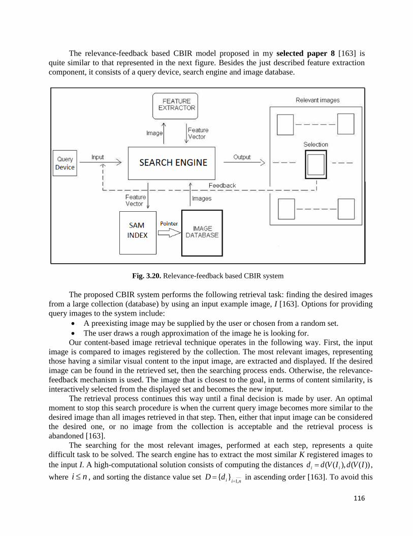
116
The relevance-feedback based CBIR model proposed in my selected paper 8 [163] is
quite similar to that represented in the next figure. Besides the just described feature extraction
component, it consists of a query device, search engine and image database.
Fig. 3.20. Relevance-feedback based CBIR system
The proposed CBIR system performs the following retrieval task: finding the desired images
from a large collection (database) by using an input example image, I [163]. Options for providing
query images to the system include:
A preexisting image may be supplied by the user or chosen from a random set.
The user draws a rough approximation of the image he is looking for.
Our content-based image retrieval technique operates in the following way. First, the input
image is compared to images registered by the collection. The most relevant images, representing
those having a similar visual content to the input image, are extracted and displayed. If the desired
image can be found in the retrieved set, then the searching process ends. Otherwise, the relevance-
feedback mechanism is used. The image that is closest to the goal, in terms of content similarity, is
interactively selected from the displayed set and becomes the new input.
The retrieval process continues this way until a final decision is made by user. An optimal
moment to stop this search procedure is when the current query image becomes more similar to the
desired image than all images retrieved in that step. Then, either that input image can be considered
the desired one, or no image from the collection is acceptable and the retrieval process is
abandoned [163].
The searching for the most relevant images, performed at each step, represents a quite
difficult task to be solved. The search engine has to extract the most similar K registered images to
the input I. A high-computational solution consists of computing the distances ))((),(( IVdIVdd ii ,
where ni , and sorting the distance value set niidD
,1}{
in ascending order [163]. To avoid this

117
costly approach, that searching task must be treated as a K-Nearest Neighbor Search problem. The
K-NN search is a generalization of the Nearest Neighbor search, a problem that can be solved by
using Spatial Access Methods.
For this reason, a SAM-based image indexing structure should be added to the retrieval
scheme, as in Fig. 3.20. The index can be modeled as a search tree data structure, whose nodes
contain feature vectors. A successfully NN search can be performed using a space-partitioning tree
structure, such as VP-tree or K-D tree. The nearest point to V(I) from the feature vector space is
thus determined, then the next closest one is identified, and so on, until the K-NNS problem is
solved. Obviously, the determined closest K feature vector points correspond to the most relevant K
images.
The proposed content-based image retrieval technique has been successfully tested on several
image databases, containing thousands of [384 x 256] digital images with different contents. We
have performed hundreds experiments, each of them being related to a different input query image,
and achieved satisfactory retrieval results (see [163]). Our CBIR system provides high values for
the performance parameters Precision and Recall, of approximately 85%. Also, it provides much
better image retrieval results than the previously described color-based retrieval approaches,
because the Gabor filter-based 3D feature vectors represent more powerful content descriptors than
the histogram-based feature vectors.
In our experiments we usually set K = 5, the number of relevant images retrieved at each
step. One of the image retrieval tests is described in the next figures. Let us assume we are
interested in an image depicting a herd of horses. We select the input image I, representing a user-
made drawing of a horse and displayed in Fig. 3.21.
The set of relevant images obtained for this query image is displayed in Fig. 3.22. They are
ranked in order of their similarity to I, a lower label number indicating a greater content similarity.
As one can see in the figure, almost all the retrieved images are depicting horses, the only
exception being the last one. We are searching for images containing more horses, so the optimal
image to be selected as an input for the new retrieval step is the fourth one, marked by a red
rectangle in the figure.
Fig. 3.21. User-made drawing used as query image
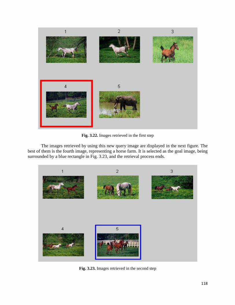
118
Fig. 3.22. Images retrieved in the first step
The images retrieved by using this new query image are displayed in the next figure. The
best of them is the fourth image, representing a horse farm. It is selected as the goal image, being
surrounded by a blue rectangle in Fig. 3.23, and the retrieval process ends.
Fig. 3.23. Images retrieved in the second step
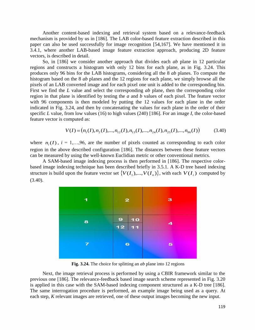
119
Another content-based indexing and retrieval system based on a relevance-feedback
mechanism is provided by us in [186]. The LAB color-based feature extraction described in this
paper can also be used successfully for image recognition [54,167]. We have mentioned it in
3.4.1, where another LAB-based image feature extraction approach, producing 2D feature
vectors, is described in detail.
So, in [186] we consider another approach that divides each ab plane in 12 particular
regions and constructs a histogram with only 12 bins for each plane, as in Fig. 3.24. This
produces only 96 bins for the LAB histograms, considering all the 8 ab planes. To compute the
histogram based on the 8 ab planes and the 12 regions for each plane, we simply browse all the
pixels of an LAB converted image and for each pixel one unit is added to the corresponding bin.
First we find the L value and select the corresponding ab plane, then the corresponding color
region in that plane is identified by testing the a and b values of each pixel. The feature vector
with 96 components is then modeled by putting the 12 values for each plane in the order
indicated in Fig. 3.24, and then by concatenating the values for each plane in the order of their
specific L value, from low values (16) to high values (240) [186]. For an image I, the color-based
feature vector is computed as:
)(),...,(),(),...,(),(),...,(),()( 962524131221 InInInInInInInIV (3.40)
where )(Ini, i = 1,…,96, are the number of pixels counted as corresponding to each color
region in the above described configuration [186]. The distances between these feature vectors
can be measured by using the well-known Euclidian metric or other conventional metrics.
A SAM-based image indexing process is then performed in [186]. The respective color-
based image indexing technique has been described briefly in 3.5.1. A K-D tree based indexing
structure is build upon the feature vector set )(),...,( 1 nIVIV , with each )( iIV computed by
(3.40).
Fig. 3.24. The choice for splitting an ab plane into 12 regions
Next, the image retrieval process is performed by using a CBIR framework similar to the
previous one [186]. The relevance-feedback based image search scheme represented in Fig. 3.20
is applied in this case with the SAM-based indexing component structured as a K-D tree [186].
The same interrogation procedure is performed, an example image being used as a query. At
each step, K relevant images are retrieved, one of these output images becoming the new input.
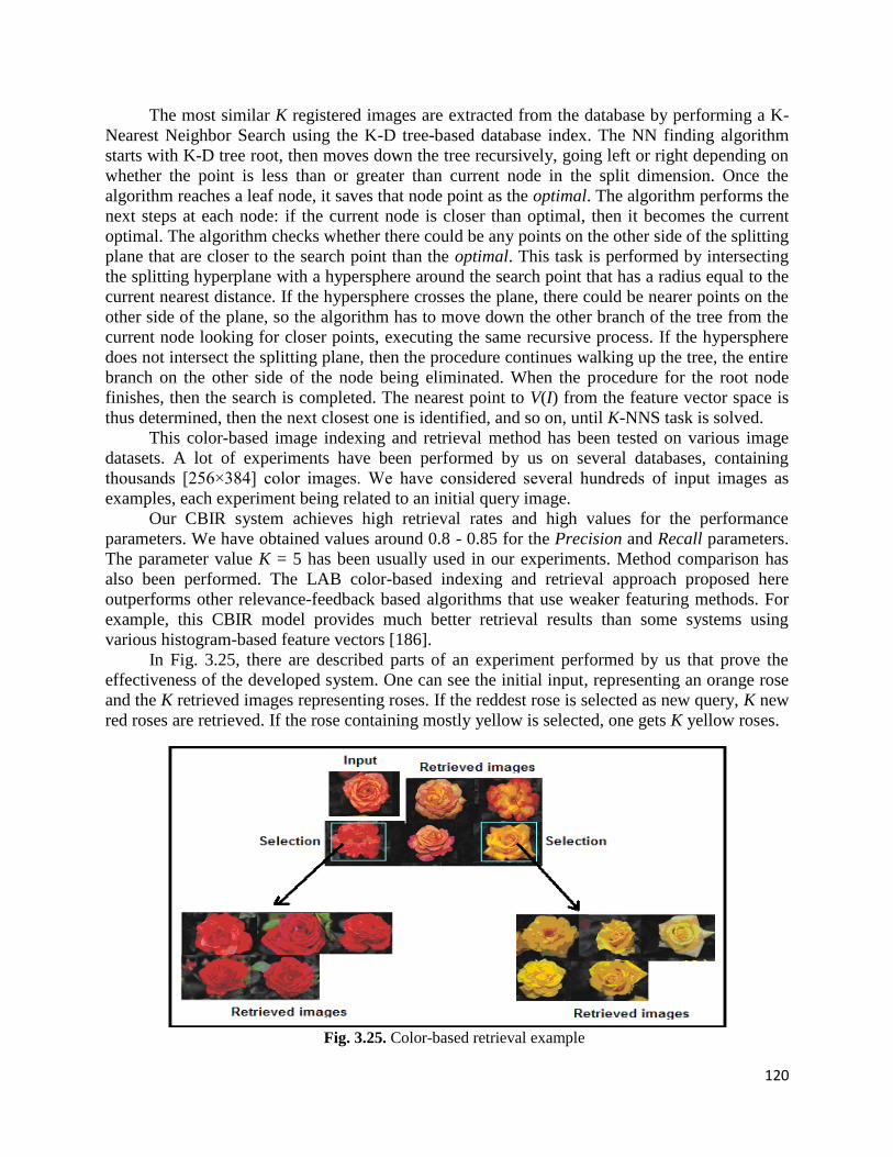
120
The most similar K registered images are extracted from the database by performing a K-
Nearest Neighbor Search using the K-D tree-based database index. The NN finding algorithm
starts with K-D tree root, then moves down the tree recursively, going left or right depending on
whether the point is less than or greater than current node in the split dimension. Once the
algorithm reaches a leaf node, it saves that node point as the optimal. The algorithm performs the
next steps at each node: if the current node is closer than optimal, then it becomes the current
optimal. The algorithm checks whether there could be any points on the other side of the splitting
plane that are closer to the search point than the optimal. This task is performed by intersecting
the splitting hyperplane with a hypersphere around the search point that has a radius equal to the
current nearest distance. If the hypersphere crosses the plane, there could be nearer points on the
other side of the plane, so the algorithm has to move down the other branch of the tree from the
current node looking for closer points, executing the same recursive process. If the hypersphere
does not intersect the splitting plane, then the procedure continues walking up the tree, the entire
branch on the other side of the node being eliminated. When the procedure for the root node
finishes, then the search is completed. The nearest point to V(I) from the feature vector space is
thus determined, then the next closest one is identified, and so on, until K-NNS task is solved.
This color-based image indexing and retrieval method has been tested on various image
datasets. A lot of experiments have been performed by us on several databases, containing
thousands [256×384] color images. We have considered several hundreds of input images as
examples, each experiment being related to an initial query image.
Our CBIR system achieves high retrieval rates and high values for the performance
parameters. We have obtained values around 0.8 - 0.85 for the Precision and Recall parameters.
The parameter value K = 5 has been usually used in our experiments. Method comparison has
also been performed. The LAB color-based indexing and retrieval approach proposed here
outperforms other relevance-feedback based algorithms that use weaker featuring methods. For
example, this CBIR model provides much better retrieval results than some systems using
various histogram-based feature vectors [186].
In Fig. 3.25, there are described parts of an experiment performed by us that prove the
effectiveness of the developed system. One can see the initial input, representing an orange rose
and the K retrieved images representing roses. If the reddest rose is selected as new query, K new
red roses are retrieved. If the rose containing mostly yellow is selected, one gets K yellow roses.
Fig. 3.25. Color-based retrieval example

121
3.6. Image and video object detection and tracking solutions
In this chapter we present our recent research results in some important and strongly-
related computer vision domains, such as object detection and tracking. Object detection
represents a high-interest computer vision research area that can be divided into two sub-
domains: image object detection and video object detection. Also, video object detection is
closely related to another important computer vision field that is video object tracking.
We describe each of these three areas in the next subsections, insisting upon our
contributions in these domains. The image object detection approaches proposed by us are
described in 3.6.1. Our results in the video object detection field are presented in 3.6.2, while the
proposed object tracking algorithms are discussed in 3.6.3.
3.6.1. Automatic image object detection techniques
Image object detection represents the computer vision process that deals with locating
semantic objects in static images. A sub-domain of object detection is object-class detection,
which aim to locate semantic objects from a certain class, such as humans, vehicles, buildings or
animals.
Many image object detection approaches have been proposed in the last decades. They can
be divided into several main categories: point-based, segmentation-based and supervised
learning based techniques [192]. The methods from the first category are based on point
detectors, like Moravec detector [193], Harris detector [194] and SIFT [84]. The segmentation-
based detection techniques use the image segments, obtained by edge-based methods,
color/texture-based algorithms [195], Active Contours [124,138] and other segmentation
approaches, for semantic image object detection. Object detection is also performed by using
some well-known supervised learning techniques. We have to mention here the Adaptive
Boosting algorithms, such as AdaBoost [196], LPBoost or GentleBoost, and Support Vector
Machines (SVM) [197], which provide very good image object detection results.
We have approached the object detection domain, developing both segmentation-based
and supervised learning-based techniques. Also, some object-class detection approaches have
been proposed [53,168,198].
The variational PDE image segmentation technique described in 3.1.2, and representing
the level-set based object contour tracking model proposed in [134], constitutes an effective
image object detection approach. We also developed an object detection method based on
color/texture-based segmentation [126]. So, the moment-based image segmentation proposed in
[126] and described in 3.1.1 can be applied successfully to image object detection. The various
combinations of the segmented regions produce the image objects [33]. These objects could be
categorized as semantic or non-semantic by performing some recognition processes on them. So,
a supervised recognition technique, using a training set that contains semantic objects, can be
applied to the input image objects, which are thus associated to some proper semantic object
classes [33].
We have investigated the object-class detection domain, developing some robust detection
techniques for several classes of image objects, such as faces, human skin and human cells. Each
of them will be detailed in this subsection.
Face detection represents a computer technology that determines the locations and sizes of
human faces in arbitrary digital images, constituting a very important image object detection sub-
domain. The main application area of face detection is biometric authentication, face finding

122
being considered the first step of facial recognition [53]. Video surveillance represents another
important application area of face detection [51].
The face detection approaches can be divided into the following categories: knowledge-
based techniques, feature-based methods, appearance-based approaches and template matching
methods. The knowledge-based methods encode human knowledge of what constitutes a typical
face, usually the relationships between facial features. A face is modeled using a set of coded
rules that are used to guide the face search process. [199]. The feature based approaches aim to
detect invariant face features, which are structural features that exist even when the pose,
viewpoint or lighting conditions vary. Let us mention here the Random Graph Matching based
approaches [200] and the Feature Grouping techniques [201]. Appearance-based techniques
train various classifiers, like Multilayer Perceptrons [202], HMM [203], Bayes classifiers [204],
SVM, Sparse Network of Winnows (SNoW) [205], PCA and Adaptive Boosting [206].
The template matching based techniques use stored face templates [207]. Usually, these
approaches use correlation operations to locate faces in images. The templates are hand-coded,
not learned and must be created for different poses. A template matching-based face detection
technique for color images is also proposed in my selected paper 9 [168]. It also performs
human skin detection and uses the identified skin regions for face detection.
Human skin color represents a useful face detection tool [207]. Our skin-based face
finding approach identifies the skin regions of the image, then determines those of them
representing faces. Besides face detection, there exist other important application areas of skin
detection, such as image content filtering and finding illegal internet content [208], content-
aware video compression or image color balancing. Numerous skin color localization techniques
have been developed in the last two decades. An influential skin detection model is the algorithm
proposed by Fleck and Forsyth in 1996 that uses a skin filter [208].
While it is one of the most used color spaces for image data processing and storing, RGB
is not a favorable choice for skin color analysis, because of the high correlation of its 3 channels
and the mixing of luminance and chrominance data [168,198]. For this reason, most skin
segmentation algorithms work with other color spaces. In [198] we propose a skin detection
technique using the HSV and YCr Cb color spaces. The RGB image is converted into the Hue
Saturation Value format, by computing the three components using the known conversion
equations. We obtain the components, H, S and V, as 3 matrices with coefficients in the [0,1]
interval. We are interested mainly in the hue value, H.
The YCr Cb color model represents a family of color spaces. In fact, it is not an absolute
color space, but a way of encoding the RGB information. In this format Y represents the
luminance, while Cr and Cb are the blue-difference and red-difference chroma components. These
3 components of the color space are computed as linear combinations of R, G and B values. The
computation formulas of the chroma components have the general form α·R+β·G+γ·B+128,
where α, β, γ ∈ [-0.5, 0.5]. We choose empirically some proper values for α, β, γ and get:
{𝐶𝑟 = 0.15 ∙ 𝑅 − 0.3 ∙ 𝐺 + 0.45 ∙ 𝐵 + 128
𝐶𝑏 = 0.45 ∙ 𝑅 − 0.35 ∙ 𝐺 − 0.07 ∙ 𝐵 + 128 (3.41)
Our method defines explicitly the skin-colored segments, by applying a set of restrictions
on these 2 components and on the hue, to determine the skin regions. Thus, we have determined
a skin related interval for each component. In our approach, each pixel of the image I belongs to
a human skin segment if the corresponding values in Cr, Cb and H are situated in those intervals.

123
One constructs a binary image Sk, having the same size as I, whose white regions
correspond to the skin segments. The proposed skin segmentation process is modeled as follows:
𝑆𝑘(𝑖, 𝑗) = {1, 𝑖𝑓 𝐶𝑟(𝑖, 𝑗) ∈ [150,165] ∝ 𝐶𝑏(𝑖, 𝑗) ∈ [145,190] ∝ 𝐻(𝑖, 𝑗) ∈ [0.02,0.1]
0, 𝑜𝑡ℎ𝑒𝑟𝑤𝑖𝑠𝑒 (3.42)
where 𝑖 ∈ [1, 𝑀] and 𝑗 ∈ [1, 𝑁], I representing a [𝑀 × 𝑁] image. The connected components of
Sk represent the detected skin regions [168]. The proposed detection method provides very good
results, although some skin identification errors could appear, because of some skin-colored
regions not representing real skin. In Fig. 3.26 (a), there is displayed an RGB image depicting
human persons. The result of the HSV conversion is displayed in Fig. 3.26 (b), while the
obtained skin detection result is depicted in Fig. 3.27. See [168] and [198] for more results.
Fig. 3.26. Digital color image conversion: RGB to HSV
Fig. 3.27. Skin detection result

124
The detected skin regions are then used in the face identification process. For each skin
segment one must decide if it represents a face, or not. First, several necessary pre-processing
operations are performed. A task that has to be solved is the separation of faces from adjacent or
occluding skin regions. Our detection task cannot identify properly the faces that are occluded by
other skin-like objects. Usually, this situation appears in group photos, like that displayed in Fig.
3.28 (a). So, we provide a separation technique involving some morphological operations
performed on the binary image Sk. Thus, we apply two successive erosions on it. First, the binary
image is eroded with a structuring element L, representing a vertical line of 5 pixels in length:
𝑆𝑘 ′ = 𝑆𝑘 ⊖ 𝐿 = ⋂ 𝑆𝑘−𝑙 (3.43)
𝑙∈𝐿
Fig. 3.28. Face separation example
Then, another erosion operation is applied on 𝑆𝑘′, by using a structuring element Sq,
representing a small square area (for example, containing a single pixel):
𝑆𝑘 ′′ = 𝑆𝑘 ′ ⊖ 𝑆𝑞 = ⋂ 𝑆𝑘 ′−𝑝 (3.44)
𝑝∈𝑆𝑞
Such a skin separation example is depicted in Fig. 3.28. In (b) the skin segments
corresponding to faces from (a) form a single connected component. The result of the
morphology-based process, given by the relations (3.43) and (3.44), is displayed on (c). The 2
greatest skin regions are clearly separated in the final binary image, 𝑆𝑘′′. Unfortunately, there
could be some situations when the face separation is not possible in the binary image. The binary
image 𝑆𝑘′′contains a set of skin segments, representing connected sequences of white pixels. Let
this set of regions be {𝑆1, … , 𝑆𝑛}. Now, we have to decide which of these regions could qualify as
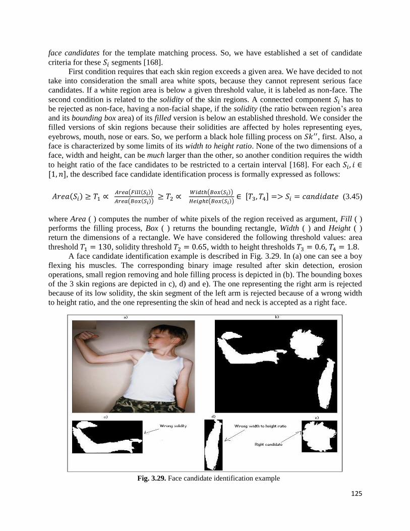
125
face candidates for the template matching process. So, we have established a set of candidate
criteria for these 𝑆𝑖 segments [168].
First condition requires that each skin region exceeds a given area. We have decided to not
take into consideration the small area white spots, because they cannot represent serious face
candidates. If a white region area is below a given threshold value, it is labeled as non-face. The
second condition is related to the solidity of the skin regions. A connected component 𝑆𝑖 has to
be rejected as non-face, having a non-facial shape, if the solidity (the ratio between region’s area
and its bounding box area) of its filled version is below an established threshold. We consider the
filled versions of skin regions because their solidities are affected by holes representing eyes,
eyebrows, mouth, nose or ears. So, we perform a black hole filling process on 𝑆𝑘′′, first. Also, a
face is characterized by some limits of its width to height ratio. None of the two dimensions of a
face, width and height, can be much larger than the other, so another condition requires the width
to height ratio of the face candidates to be restricted to a certain interval [168]. For each 𝑆𝑖, 𝑖 ∈[1, 𝑛], the described face candidate identification process is formally expressed as follows:
𝐴𝑟𝑒𝑎(𝑆𝑖) ≥ 𝑇1 ∝ 𝐴𝑟𝑒𝑎(𝐹𝑖𝑙𝑙(𝑆𝑖))
𝐴𝑟𝑒𝑎(𝐵𝑜𝑥(𝑆𝑖)) ≥ 𝑇2 ∝
𝑊𝑖𝑑𝑡ℎ(𝐵𝑜𝑥(𝑆𝑖))
𝐻𝑒𝑖𝑔ℎ𝑡(𝐵𝑜𝑥(𝑆𝑖))∈ [𝑇3, 𝑇4] => 𝑆𝑖 = 𝑐𝑎𝑛𝑑𝑖𝑑𝑎𝑡𝑒 (3.45)
where Area ( ) computes the number of white pixels of the region received as argument, Fill ( )
performs the filling process, Box ( ) returns the bounding rectangle, Width ( ) and Height ( )
return the dimensions of a rectangle. We have considered the following threshold values: area
threshold 𝑇1 = 130, solidity threshold 𝑇2 = 0.65, width to height thresholds 𝑇3 = 0.6, 𝑇4 = 1.8.
A face candidate identification example is described in Fig. 3.29. In (a) one can see a boy
flexing his muscles. The corresponding binary image resulted after skin detection, erosion
operations, small region removing and hole filling process is depicted in (b). The bounding boxes
of the 3 skin regions are depicted in c), d) and e). The one representing the right arm is rejected
because of its low solidity, the skin segment of the left arm is rejected because of a wrong width
to height ratio, and the one representing the skin of head and neck is accepted as a right face.
Fig. 3.29. Face candidate identification example
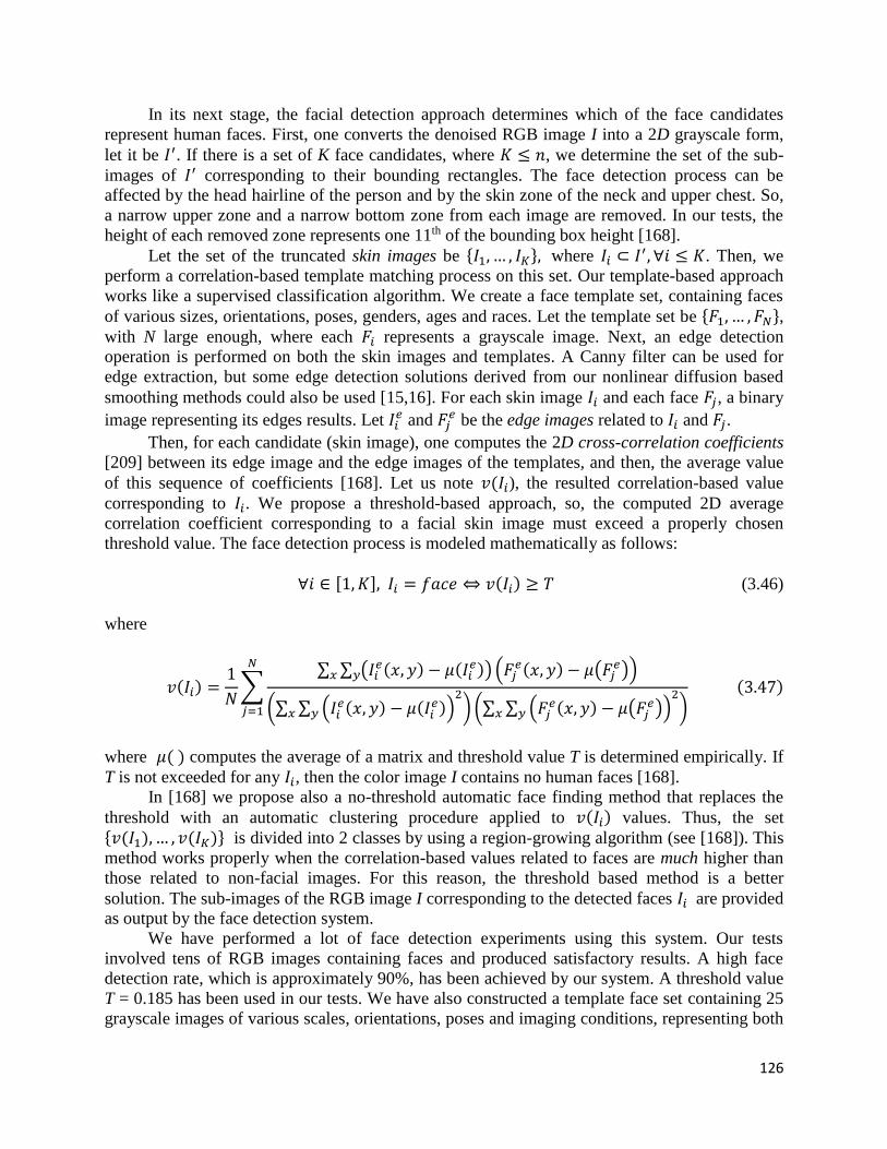
126
In its next stage, the facial detection approach determines which of the face candidates
represent human faces. First, one converts the denoised RGB image I into a 2D grayscale form,
let it be 𝐼′. If there is a set of K face candidates, where 𝐾 ≤ 𝑛, we determine the set of the sub-
images of 𝐼′ corresponding to their bounding rectangles. The face detection process can be
affected by the head hairline of the person and by the skin zone of the neck and upper chest. So,
a narrow upper zone and a narrow bottom zone from each image are removed. In our tests, the
height of each removed zone represents one 11th of the bounding box height [168].
Let the set of the truncated skin images be {𝐼1, … , 𝐼𝐾}, where 𝐼𝑖 ⊂ 𝐼′, ∀𝑖 ≤ 𝐾. Then, we
perform a correlation-based template matching process on this set. Our template-based approach
works like a supervised classification algorithm. We create a face template set, containing faces
of various sizes, orientations, poses, genders, ages and races. Let the template set be {𝐹1, … , 𝐹𝑁},
with N large enough, where each 𝐹𝑖 represents a grayscale image. Next, an edge detection
operation is performed on both the skin images and templates. A Canny filter can be used for
edge extraction, but some edge detection solutions derived from our nonlinear diffusion based
smoothing methods could also be used [15,16]. For each skin image 𝐼𝑖 and each face 𝐹𝑗, a binary
image representing its edges results. Let 𝐼𝑖𝑒 and 𝐹𝑗
𝑒 be the edge images related to 𝐼𝑖 and 𝐹𝑗.
Then, for each candidate (skin image), one computes the 2D cross-correlation coefficients
[209] between its edge image and the edge images of the templates, and then, the average value
of this sequence of coefficients [168]. Let us note 𝑣(𝐼𝑖), the resulted correlation-based value
corresponding to 𝐼𝑖. We propose a threshold-based approach, so, the computed 2D average
correlation coefficient corresponding to a facial skin image must exceed a properly chosen
threshold value. The face detection process is modeled mathematically as follows:
∀𝑖 ∈ [1, 𝐾], 𝐼𝑖 = 𝑓𝑎𝑐𝑒 ⇔ 𝑣(𝐼𝑖) ≥ 𝑇 (3.46)
where
𝑣(𝐼𝑖) =1
𝑁∑
∑ ∑ (𝐼𝑖𝑒(𝑥, 𝑦) − 𝜇(𝐼𝑖
𝑒)) (𝐹𝑗𝑒(𝑥, 𝑦) − 𝜇(𝐹𝑗
𝑒))𝑦𝑥
(∑ ∑ (𝐼𝑖𝑒(𝑥, 𝑦) − 𝜇(𝐼𝑖
𝑒))2
𝑦𝑥 ) (∑ ∑ (𝐹𝑗𝑒(𝑥, 𝑦) − 𝜇(𝐹𝑗
𝑒))2
𝑦𝑥 ) (3.47)
𝑁
𝑗=1
where 𝜇( ) computes the average of a matrix and threshold value T is determined empirically. If
T is not exceeded for any 𝐼𝑖, then the color image I contains no human faces [168].
In [168] we propose also a no-threshold automatic face finding method that replaces the
threshold with an automatic clustering procedure applied to 𝑣(𝐼𝑖) values. Thus, the set {𝑣(𝐼1), … , 𝑣(𝐼𝐾)} is divided into 2 classes by using a region-growing algorithm (see [168]). This
method works properly when the correlation-based values related to faces are much higher than
those related to non-facial images. For this reason, the threshold based method is a better
solution. The sub-images of the RGB image I corresponding to the detected faces 𝐼𝑖 are provided
as output by the face detection system.
We have performed a lot of face detection experiments using this system. Our tests
involved tens of RGB images containing faces and produced satisfactory results. A high face
detection rate, which is approximately 90%, has been achieved by our system. A threshold value
T = 0.185 has been used in our tests. We have also constructed a template face set containing 25
grayscale images of various scales, orientations, poses and imaging conditions, representing both

127
male and female faces, and people of various ages and races, some of them having structural
elements. The template set can be extended, by adding new faces, but while a large set may
improve the detection results, it also produces a high computation complexity. Our approach
produces a low number of false negatives (missed faces) and very few false positive (non-facial
image regions detected as faces), which means high values for the performance parameters
Precision and Recall. The performances of the proposed face detection system are comparable
with those of the face detection techniques mentioned in introduction. It achieves better detection
results for frontal faces, than for faces characterized by various orientations.
Fig. 3.30. Facial template set
A face detection example is displayed in the next figure. The skin detection process
depicted in Fig. 3.26 and Fig. 3.27 is continued with the face detection process represented in
Fig. 3.31. In (a) there are displayed the main skin regions obtained by performing the
morphological operations, hole filling and small region removing on the binary image from Fig.
3.27. One of them is rejected because of its low solidity, the remaining regions being accepted as
128
face candidates, as one can see in (b). The template matching process is performed by using the
template face set represented in Fig. 3.30. One can see the resulted average correlation
coefficient values in (c), those greater than the threshold (0.185) corresponding to the detected
faces, which are surrounded by black rectangles in that grayscale image. The final face detection
result for the RGB image is displayed in (d), the human faces being marked by red bounding
boxes [168].
Fig. 3.31. Face detection example

129
Another object-class detection technique developed by us represents a human cell
detection algorithm [210]. Although our detection approach aims to locate cells in static images
and video frames, it could be used successfully to detect other image object classes, such as
humans or vehicles. The proposed object detection model uses a sliding-window based object
searching approach, a HOG-based feature extraction and a SVM-based feature vector
classification technique.
Histograms of Oriented Gradients (HOG) represent a robust feature descriptor used in the
computer vision domain for object detection. They prove to be very useful for human detection
[211], but we use them successfully for cell featuring in this work [210]. We compute HOG
characteristics for the sub-images corresponding to the cells’ bounding boxes. A HOG-based
feature vector is modeled for such an image [210]. First, one determines the image gradient
values, representing directional changes in the intensity or color. The gradient vector is formed
by combining the partial derivatives of the image I in the x and y directions:
,,
y
I
x
II (3.48)
The gradients in the two directions can be computed by applying the 1D centered, point
discrete derivative mask in the horizontal and vertical directions:
TI
y
I
Ix
I
1 0 1
1 0 1
(3.49)
The gradient orientations of the image are computed as
y
I
x
I,arctan . The image
I is then divided into cells, and for each cell, one computes a local 1D histogram of gradient
directions (orientations) over the pixels from that cell [210,211]. We consider 9 bins for the local
histogram. The histogram channels are evenly spread over 0 to 180 degrees, so each histogram
bin corresponds to a 20 degree orientation interval. The obtained cell histograms are then
combined into a descriptor vector of the image [210].
First, these cells have to be locally contrast-normalized, due to the variability of
illumination and shadowing in the image. That requires grouping the cells together into larger,
spatially-connected blocks. Once the normalization is performed, all the histograms can be
concatenated in a single feature vector, representing the HOG descriptor. We use [3x3] cell
blocks of [6x6] pixel cells with 9 histogram channels. The feature vector of the image is
computed as its HOG descriptor, having 81 coefficients. This could be expressed as
)()( IHOGIV [210]. The detection process uses a supervised classification of these feature
vectors, which is performed through a SVM-based approach.
Support Vector Machines (SVM) represent supervised machine learning models, widely
used in object detection tasks [197]. They can perform efficiently both linear and non-linear
feature vector classification. Using a set of training examples, each marked as belonging to one
of two classes, a SVM training algorithm predicts, for each given input, which of two possible
classes must represent the correct output [197].

130
Any image object-class detection task can be formulated as a binary linear classifier
problem. It can be solved by considering two classes, containing objects and non-objects
respectively, then applying a SVM on them. We develop a non-linear SVM training model for
human cell detection, because non-linear SVMs are consistently found to be better suited for the
object detection task [197,210].
The training image set constructed by us contains the following two subsets: the set of
positives, containing bounding rectangles of biological cells, and the set of negatives, containing
non-cell images of various sizes. A training set example is described in the next figure. Its
positive samples are displayed in Fig. 3.32 (a), while the negative samples are represented in Fig.
3.32 (b).
Fig. 3.32. The training set of the system
The training set could be expressed in the following form:
1,1 ,,,...,, i11 xxTxTS nn (3.50)
where iT represent the training samples, and their labels are:
negativeT
positiveTTxx
i
i
i if ,1
if ,1)( i (3.51)
131
The described HOG-based feature extraction is performed on these training subsets, the
system’s feature training set being composed of the feature vectors niTV i ,...,1),( . One must
identify the maximum-margin hyperplane that divides the objects characterized by 1i x from
those having 1 i x . We consider a quadratic programming technique to separate hyperplane
identification [210]. Also, our non-linear classification algorithm uses a nonlinear kernel
function instead of the dot product used in the linear case. So, a quadratic kernel is considered to
map the training data S into the kernel space. If this SVM classifier is applied to an input object
represented by its bounding image I, the SVM-based classification of its feature vector will
produce the object labeling that can be expressed formally as: x(I) = SVM (V(I)).
One has to solve the following computer vision task: locate all objects representing human
cells from a given image Im. We detect the bounding boxes of those cells by performing a
sliding-window scanning over the grayscale version of the respective image [210]. We propose a
cell search algorithm that scans Im using a variable sized sliding window. At each step, one
computes the HOG-based feature vector of the sub-image corresponding to current window. The
SVM classification algorithm is then applied to the feature vector, the analyzed sub-image being
labeled as either positive or negative [210]. We introduce the following condition: if a positive is
identified, the next search must be performed far enough from it. So, the positions of pixels of
the detected cell are marked as visited, this approach reducing the searching complexity [210].
We consider that the widths and heights of the cells vary between some minimum and
maximum values,maxminmaxmin ,,, hhww , so, the sliding-window size has to vary accordingly. Let
us note Subim(Im, x, y, w1, w2 , h1, h2) the set of all subimages of Im having the upper-left pixel
Im(x,y), the width in interval [w1, w2] and the height in [h1, h2]. This set of subimages can be
determined recursively. We construct a searching algorithm expressed by next pseudocode [210]:
Detect_cells (Im)
S ; mark = 0 matrix with the same size NM as Im;
for i = 1 to M - hmin
for j = 1 to N - wmin
if mark (i, j) = 0
for each ),,,,,,( maxminmaxmin hhwwjiImSubimI
Compute V (I) = HOG(I);
Apply SVM classifier to V(I): x(I) = SVM(V(I));
if x(I) = 1 then
ISS ;
for each pixel location I (a,b)
mark(a,b) = 1; (mark location as visited)
end
end
end
end
end
end
Return S.

132
The result of a cell searching process is displayed in Fig. 3.33. The stem cells from the
grayscale image are identified and marked with red rectangles. In that figure, one can see also a
blue rectangle marking a subimage representing a non-cell example.
Fig. 3.33. Example of a cell detection result
We have performed many cell detection experiments using the proposed technique. The
numerical tests performed on hundreds images, containing various types of cells, have produced
satisfactory detection results that prove the effectiveness of our method. It has achieved a high
detection rate, of approximately 90%, and also, high values are obtained for the performance
parameters. We get values around 0.9 for both the Precision and Recall parameters. Therefore,
almost all the detected objects returned by our approach are relevant, very few false positives
being returned. Also, the high Recall value indicates that almost all true positives are returned.
We have developed and tested many appropriate SVM training sets, containing cells and
non-cell objects. One of those training data sets is described in Fig. 3.31 being composed of 29
positives and 29 negatives. While the proposed detection technique provides satisfactory cell
identification results, it does not execute fast enough. That is because of the high complexity and
computational cost of the sliding-window based search algorithm. In our tests we apply this
algorithm with the parameters 50,20,50,20 maxminmaxmin hhww , M = 512 and N = 672.
Lower values may reduce its complexity, but also its effectiveness. The values of parameters
related to HOG computing, also may influence the computational complexity of the detection.
Method comparisons have also been performed. Thus, our object searching procedure is
considerably faster than methods based on Exhaustive Search (ES), but slower than approaches
that do not perform image scanning. Thus, we have also compared the obtained detection results
with those produced by other object identification techniques that are based on image
segmentation, using edge detection or threshold values and some morphological operations
[212]. From our tests, we have found that the approach described here outperforms them,
obtaining a higher Recall value, but also it is somewhat slower. While the segmentation-based
methods often fail to return all the positives, producing a higher number of missed biological
cells, they execute faster than the approach presented here [210].

133
3.6.2. Video object detection approaches
Video object detection represents an important and challenging computer vision domain,
which is closely related to the video object tracking described in the next subsection. A video
object of a movie constitutes a sequence of image objects that represent the instances (states) of
the video object in a succession of frames of that movie. So, the video object detection process
involves locating the instances of the video objects in the frames of a video sequence.
Object detection and tracking has a wide variety of computer vision application domains. The
most important of them are the video compression, video surveillance, human-computer
interaction, video indexing and retrieval.
Numerous video object detection techniques have been developed in recent years, and they
could be divided in two categories. Video object detection can be performed using the image
object detection approaches described in 3.6.1. Thus, the image objects from each video frame
can be detected by using techniques based on active contour models [138], segmented regions
[126], Hough transforms [213], adaptive boosting or SVM. These techniques belong to the first
video object detection category.
The second category contains the video motion-based object detection approaches. Thus,
the video objects presenting the most interest are the moving objects of a video sequence and not
the static objects, whose detection reduces to image object detection. The moving object
detection techniques are based on background subtraction [214], frame-differencing [215] or
motion estimation [33].
We also proposed some moving object detection algorithms in our past papers [33,217]. A
background subtraction based video object detection technique is provided in [217]. We will not
insist here on this approach from 2005, describing in detail a more recent detection method
instead [218-220].
An automatic multiple moving object detection technique is proposed in the last selected
paper [219]. My developed model detects efficiently the video objects from a static-camera
movie by using a novel temporal differencing algorithm and several mathematical morphology-
based operations. I have also developed some video object-class detection techniques, such as
pedestrian detection [218,219] and sonar object detection approaches [220], based on this
moving object detection algorithm.
So, in [219] the video frames of the analyzed color movie are converted into the grayscale
form, the set nImIm ,...,1 being obtained. One considers a temporal differencing-based video
motion estimation approach. The difference of two consecutive frames indicates the motion
between them, the resulted non-black image zones representing the moving regions. Such a
moving region may not represent an entire image object, because both the foreground and the
background of the frame can be composed of more homogeneous regions, characterized by
various intensities. The frame difference is noted as jinji,ImImjiFd ji ],,1[ ,),( . Each
moving object present in iIm and jIm , is represented in ),( jiFd by some non-black regions.
Its high-intensity pixels (having greater values than background) are displayed in ),( jiFd at the
locations occupied in iIm , while its low-intensity pixels are displayed in ),( jiFd at their
positions in jIm . Frame difference is then converted into the binary format by setting to 1 all
pixels exceeding a properly selected threshold value, T:

134
jinji,TjiFd
TjiFdjiFdb
],,1[ ,
),(for ,0
),(for ,1),( (3.52)
A mathematical morphology based process is next applied to image ),( jiFdb . The dilation
morphological operation is very useful in this case, producing the dilated binary image as:
Sqs
sbbm jiFdSqjiFdjiFd
),(),(),(
(3.53)
where represents the dilation morphological operator and Sq is a kk structuring element
[221]. The connected components of the dilated image ),( jiFd m are then determined, those
representing errors provided by redundant noise or undesired camera motion being removed. We
consider the following connected components to be discarded: small white spots – connected
components whose area is under a low threshold; components whose bbox has a dimension
under a threshold value; low solidity components. The resulted image is noted ),( jiFd p
m[218].
The proposed detection algorithm identifies the moving objects from 1Im to
1nIm , first.
At ith step, it determines the video objects of iIm , using the next 2 frames, 1iIm and 2iIm . The
corresponding morphologically processed frame difference images )1,( iiFd p
m and )2,( iiFd p
m
are computed, and their intersection is then determined as:
],)[2,(],)[1,(for ,0
],)[2,(],)[1,(for ],,)[1,(],))[2,()1,((
yxiiFdyxiiFd
yxiiFdyxiiFdyxiiFdyxiiFdiiFd
p
m
p
m
p
m
p
m
p
mp
m
p
m (3.54)
The connected components of the intersection )2,()1,( iiFdiiFd p
m
p
m correspond to all
high-intensity regions of the moving objects from iIm . The low-intensity components of its
moving objects are determined by using a similar procedure. They correspond to the connected
components of ),2(),1( iiFdiiFd p
m
p
m . The moving objects of iIm are detected by computing
the next sum of image intersections:
)),2(),1(())2,()1,(()( iiFdiiFdiiFdiiFdiOb p
m
p
m
p
m
p
m (3.55)
The connected components of the binary image Ob(i) correspond to the moving objects of
the frame iIm . The last step of the detection task consists of the localization of these objects in
nIm . We apply a backward identification process that is modeled as follows:
)),2(),1(())2,()1,(()( nnFdnnFdnnFdnnFdnOb p
m
p
m
p
m
p
m (3.56)
Each binary image Ob (i) contains the same number of connected components. For each
component, one identifies its bounding box. The sub-images of frame iIm corresponding to these
bounding rectangles represent its moving objects (foreground) (see [219]). Such a foreground
detection example is represented in Fig. 3.34.
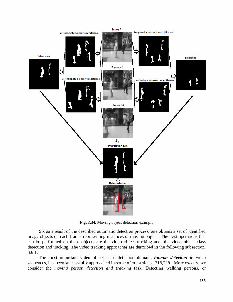
135
Fig. 3.34. Moving object detection example
So, as a result of the described automatic detection process, one obtains a set of identified
image objects on each frame, representing instances of moving objects. The next operations that
can be performed on these objects are the video object tracking and, the video object class
detection and tracking. The video tracking approaches are described in the following subsection,
3.6.1.
The most important video object class detection domain, human detection in video
sequences, has been successfully approached in some of our articles [218,219]. More exactly, we
consider the moving person detection and tracking task. Detecting walking persons, or

136
pedestrians, in video images represents a very challenging task, complicated by various factors,
like camera position, variable people appearance, wide range of poses adopted by human beings,
variations in brightness, illumination, contrast levels or backgrounds, and person occlusions
[222].
Over the last decade the problem of detecting and tracking humans has received a very
considerable interest. Significant research has been devoted to detecting, locating and tracking
people in videos, since many applications involve persons’ locations and movements [222].
Also, human detection and tracking has a wide variety of computer vision application areas, the
most important of them being video surveillance and security systems, biometrics, law
enforcement, human-computer interaction (HCI), video indexing and retrieval, medical imaging,
robotics and augmented reality.
Our proposed approach decides which of the detected moving objects represent
pedestrians. We set several conditions related to human body that have to be satisfied by each
object representing a pedestrian. The first condition is that the height of the bounding rectangle
of the image object representing a human must be at least two times greater than its width. The
second condition is that the object solidity has to be over 50%. If inobob ,...,1 are the objects
corresponding to )(iOb , and )(),...,( 1 inobIobI the set of their sub-images, the above conditions
can be formalized as follows:
i
jjj
jjnj
obAreaobwobh
obwobh,1 ,
2)()(
2
(3.57)
where jobh and jobw are the height and the width of image )( jobI . Let )()( iObiObj
the binary image containing the connected components satisfying (3.57) only.
Our third condition is related to the presence of skin regions. So, any video object must
contain skin regions to be considered a moving person [218]. A skin detection process is
performed on each video frame. Some skin identification techniques based on explicitly defined
skin segments, therefore working similarly to the skin detection model described in 3.6.1 [198],
are introduced for this purpose [218].
For each frame iI we get a binary image iIS , that is similar to Sk given by (3.42), whose
connected components correspond to its skin regions. If these skin segments are identified in the
moving object locations, then those objects must represent humans. So, for each i, our approach
computes the intersection iISiObj )( and determines its connected components. The
moving objects containing these components are considered pedestrians [218,219].
A pedestrian detection example is described in Fig. 3.35. In (a) one displays the moving
object detection result for a given frame. The skin segmentation result for that color frame is
provided in (b). Obviously, the skin regions in (b) are located within the red bounding rectangles
from (a). Also, the two moving objects detected in (a) satisfy the conditions related to width to
height ratio and solidity. So, the detected moving video objects represent walking persons. The
moving object detection example from Fig. 3.34 leads also to a pedestrian detection result, the
two detected image objects representing human beings.
While our human detection approach works successfully for identification of non-occluded
side view pedestrians [223], it performs somewhat weaker on occluded people [224], front-view

137
or rear-view moving people. Also, it is not appropriate for non-pedestrian human detection and
cannot locate persons that are not moving in upright position.
Fig. 3.35. Pedestrian detection example
An automatic temporal differencing based object detection technique is also used for
multiple sonar object detection in ultrasound movies [220]. The video tracking of these moving
objects is also described in 3.6.3.
The automatic character of my video object detection technique and its capability to
perform multiple moving object detection represent important advantages of the described
technique. The sensitivity to undesired camera motions represents the major limitation of this
detection approach that is well-suited for fixed camera videos. Because of the used temporal
differencing procedure, our moving object detection method is quite sensitive to camera
movements. Even the presence of a small camera motion may affect the entire object detection
process [219].
3.6.3. Video tracking methods
The video object tracking represents the video analysis process of monitoring the spatial
and temporal changes of the video object during the movie sequence, including its presence,
position, size and shape. A video tracking approach has to solve the temporal correspondence
problem that is the task of matching the target object in successive video frames [144,192].
State of the art video object tracking techniques include: mean-shift based tracking [225],
kernel tracking [192,226], statistical methods, like those based on Kalman filtering [192,227],
particle filtering [192,228] and HMM [229], object matching based tracking [230], optical flow
based tracking [231], eigentracking [232] and contour evolution based tracking. Video tracking
is often a difficult process, due to some factors such as abrupt object motion, objects’ variable
form, object occlusions, camera motion and scene illumination changes [144].
We have approached two video tracking types. The first one is based on image object
matching and uses the objects already detected in video frames. The tracking processes of the
second type begin with detecting the initial instance of the video object, then identifying that

138
image object repeatedly in subsequent frame sequence. Obviously, we consider tracking of
moving objects only, since the tracking of static video objects represents a trivial task.
The object-matching based video tracking approaches proposed by us track successfully
multiple objects across movie sequences. These methods determine the correspondences between
image objects from different frames. As a result of the multiple moving object detection process,
all image objects representing video object instances are located within movie. The tracking
process identifies for each object of the current frame, the unique object corresponding to it from
the next frame.
Let us suppose there are K detected objects on each frame, the detected object set
corresponding to iI is ],1[ ,,...,1 niObOb i
K
i , where each object i
jOb is considered in the sub-
image form. For each ],1[,1,1 Kjni one must determine the value ],1[ Kk such that 1i
kOb corresponds to i
jOb , as the next instance of the same moving object. Our tracking
approaches are based on object content similarity, therefore we have i
j
i
k ObOb 1. The next
instance of a video object must be the image object from next frame, which is most similar to the
current instance, therefore corresponding to the minimum value of a similarity metric.
So, the object matching based video tracking process becomes equivalent to a supervised
object recognition process. All the image objects i
jOb can be characterized by using the content-
based feature extraction approaches described in section 3.4. The object matching process is
modeled as follows:
],1[],1,1[ )),(),((minarg 1
],1[KjniObVObVdind i
k
i
jKk
(3.57)
where ind is the optimal value of k (index of the next instance), d represents a metric that works
properly for the feature vectors )( i
jObV . Any tracked video object is obtained an ordered
sequence of similar image objects.
The video object feature extraction could depend on the class of moving objects to be
tracked. Thus, in [220] we consider a multiple moving object detection and tracking process for
sonar movies. A 2D Gabor filter-based texture analysis is performed on the image objects that
represent video instances detected through a temporal differencing based algorithm [218-220].
Each object i
jOb is filtered with a two-dimensional Gabor filter at various orientations
(angles), radial frequencies and standard deviations. Thus, the 6-channel 2D Gabor filtering bank
]3,1[,5.1,75.01,2,, kff
iik
G , where n
kk
and ),(,,, yxG
yxik f is computed as in
(3.31), is applied to the object. A 3D feature vector )( i
jObV representing a proper content
descriptor is obtained for each object (see [220] for more).
The considered Gabor filter-based sonar object featuring produces satisfactory video
tracking results. Thus, the tracking algorithm is characterized by a high object recognition rate,
exceeding 80%. The performance parameters are Precision = 0.80, Recall = 0.85. This means
there is a small number of false positives and false negatives too. A sonar object tracking
example is provided in the next figure. There are two vehicles that are tracked in the ultrasound
movie. The two resulted moving objects are marked in red and blue, respectively.

139
Fig. 3.36. Object matching process in a sonar video
Another video object tracking task uses a HOG-based feature extraction [219]. While the
characteristics based on Histogram of Oriented Gradients are widely used for human detection in
static images, our technique uses the HOG-based features for human tracking in video images
[219].
The moving objects are detected by using the temporal differencing procedure described in
3.6.2. Then, those moving objects representing pedestrians are identified using the human body
related conditions described there [219]. An object matching process is then performed for
tracking the detected moving persons, i
jH . The feature vector of a human object is computed as
the Histogram of Oriented Gradients of its corresponding sub-image, as described in 3.6.1 [210,
211]. So, KjniHHOGHV i
j
i
j ,1,,1),()( . The Euclidean metric is used to measure the
distances between these HOG-based feature vectors having 81 coefficients.
The human matching process is performed similarly to the object matching given by
(3.57). So, the proper match for i
jH is determined as the human 1
)(
i
jindiH of the next frame,
where
KjniHVHVdjind i
t
i
jKt
i
,,)(),(minarg)( 1
,1
. Therefore, any tracked pedestrian
is obtained as a sequence ],1[)(
1
)(
2
)(
1 },...,,...,,11 Kj
n
jind
i
jindjindj niHHHH
[219].
The detected moving objects from Fig. 3.34 are then identified easily as humans. The
corresponding human tracking process is represented in Fig. 3.37. The matching is represented
by arrows linking objects from different frames and marked by the distances between their HOG-
based feature vectors. The colored arrows, corresponding to lower distance values, indicate
correct matches, while the white ones, marked by higher values, represent wrong matches. The
instances of each person are marked with the same color and linked by arrows of that color.

140
Fig. 3.37. Pedestrian tracking example
The proposed video tracking solution is characterized by a high person matching rate, of
approximately 90 %. The resulted performance parameters are Precision = 0.90, Recall = 0.85
and F1 = 0.874, which means that very few false positives and false negatives are produced by
this pedestrian tracking technique.
Another effective moving person tracking method is proposed in [218]. The pedestrians
are detected similarly in the video frames, for each iI a moving person sequence },...,1
i
K
i PP
being obtained. We consider a normalized correlation-based human matching approach for video
tracking, therefore no feature extraction process in performed [218]. Our approach computes the
2D cross-correlation coefficients between the current object (person) of the current video frame
and all the human objects of the successive frame. Its optimal match is determined as the moving
person corresponding to the maximum correlation coefficient value. So, we have:
],1[],,1[,
)(),()(),(
)(),()(),(maxarg)(
2112
11
],1[Kjni
PyxPPyxP
PyxPPyxPjmatch
x y
i
k
i
kx y
i
j
i
j
x y
i
k
i
k
i
j
i
j
Kki
(3.58)
Therefore, a tracked pedestrian could be modeled through the following sequence:
],1[)(
1
)(
2
)(
1 },...,,...,,11 Kj
n
jmatch
i
jmatchjmatchj niPPPP
[218].

141
Fig. 3.38. Correlation-based human tracking example
Another considered human matching solution uses the edges of the i
jP image objects [218],
instead of these objects in the correlation procedure given by (3.58). Unfortunately, computing
the edge information raises substantially the complexity of the video tracking process. A
correlation-based human tracking example is displayed in Fig. 3.38. On the left column one can
see the identified humans, two for each grayscale frame, bounded by colored rectangles. The
human matching process is represented by arrows linking objects of different frames and marked
by the computed 2D correlation results [218]. The arrows corresponding to the higher correlation
values indicate the correct matches. On the right column there are displayed the final tracking
results: the identified and tracked moving persons in the initial color video frames [218].
We have tested this correlation-based human tracking technique on hundreds video, getting
satisfactory results. Our tracking approach is also characterized by a high person matching rate
that exceeds 80 percent. The performance parameters are Precision = 0.85 and Recall = 0.85
[218]. Both the HOG-based and the correlation-based pedestrian matching techniques provide
comparable good tracking results and outperform other methods. From the performed method
comparisons, we have found that pixel differencing based matching approaches, like those using
SAD, MAD, MSD or various histograms, achieve poorer tracking results. Also, our human
matching models have lower time complexity than point tracking techniques [192], like those
using Kalman filters or particle filters, while producing comparable satisfactory results.
142
Let us now describe the second video object tracking type, which is not based on
previously detected objects, presenting our results. The idea of this kind of video tracking is to
select or detect a semantic image object in a given frame and then track it across subsequent
frames.
Thus, in the past we proposed some video object tracking algorithms based on motion
estimation [33,217]. In those papers some procedures for estimating the video motion or optical
flow [231], such as the block-matching algorithm, were considered. The motion vectors between
any two successive video frames are determined by applying the block-matching procedure, each
such a vector representing a pair of offsets (dx, dy) corresponding to a pixel. The next instance of
a moving object is detected easily by applying the corresponding motion vector to each pixel of
the current video object instance [33,217].
A much more important video tracking result is obtained in [233], where a robust object
tracking technique is provided. Our developed method is able to locate the instances of any video
object in a movie sequence, no matter if the movie is recorded with a fixed or moving camera
[233]. The first state of the target object could be selected interactively or determined
automatically using the image object detection approaches. Then, one detects the video object
location in the next frame, by using a sliding-window based object detector [233]. The classic
sliding-window method, consisting of a full-search and using fixed-size sliding windows, is
computationally expensive and does not treat the object scaling effect. So, we propose an object
localization approach based on a variable-sized sliding-window and an improved N-step search
algorithm [233].
Unlike other video tracking techniques, our proposed model takes into consideration not
only the object position changes, but also the possible shape and scale transformations. The
object scaling aspect is treated using a variable sized sliding-window while the object translation
is approached using a template matching based on an N-Step Search algorithm. Since any object
in a frame cannot differ much in shape and size from its state in the previous frame, the values of
the width and height of that object’s bbox must be situated in some neighborhood intervals of the
width and height of its previous state. In [233] there is provided an algorithm that locates all
image objects determined by these intervals. It works as applying a variable-sized sliding-
window on a object’s neighborhood. So, one has to determine all objects modeled as following:
sObylObxtObykObxOb lstk )(,)(,)(,)( 2211,,, , (3.59)
where the current object is codified by the coordinates of the upper-left and bottom-right corners
as )(),(),(),( 2211 ObyObxObyObxOb ,
],[, MMlk , ],[, NNst , and 0, NM represent
quite small number of pixels. All image objects modeled by (3.59) contain the next sub-image:
NObyMObxNObyMObxOb NM )(,)(,)(,)( 2211, (3.60)
So, the set of needed objects is composed of NMOb , , the objects containing NMOb , padded
with an upper zone, those containing NMOb , padded with a bottom zone, those containing NMOb ,
padded with a left zone and those containing NMOb , padded with a right zone. In [233] one
provides a recursive object locating algorithm, in pseudo-code, that is applied to NMOb ,
and
produces )( ,NMObS , which is the set of objects lstkOb ,,, .
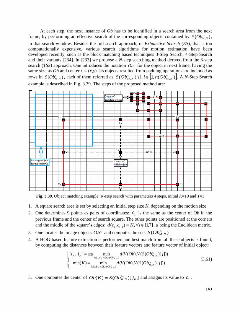
143
At each step, the next instance of Ob has to be identified in a search area from the next
frame, by performing an effective search of the corresponding objects contained by )( ,NMObS ,
in that search window. Besides the full-search approach, or Exhaustive Search (ES), that is too
computationally expensive, various search algorithms for motion estimation have been
developed recently, such as the block matching based techniques 3-Step Search, 4-Step Search
and their variants [234]. In [233] we propose a N-step searching method derived from the 3-step
search (TSS) approach. One introduces the notation cOb for the object in next frame, having the
same size as Ob and center c = (x,y). Its objects resulted from padding operations are included as
rows in )( ,
c
NMObS , each of them referred as )(,1 ],)[( ,,
c
NM
c
NM ObniiObS . A N-Step Search
example is described in Fig. 3.39. The steps of the proposed method are:
Fig. 3.39. Object matching example: N-step search with parameters 4 steps, initial K=10 and T=1
1. A square search area is set by selecting an initial step size K, depending on the motion size
2. One determines 9 points as pairs of coordinates: 1c is the same as the center of Ob in the
previous frame and the center of search square. The other points are positioned at the corners
and the middle of the square’s edges: ]7,1[ ,),( 1 iKccd ii , d being the Euclidean metric.
3. One locates the image objects icOb and computes the sets )( ,
ic
NMObS .
4. A HOG-based feature extraction is performed and best match from all these objects is found,
by computing the distances between their feature vectors and feature vector of initial object:
])))[((),((min)min(
])))[((),((minarg],[
,](,1[],9,1[
,](,1[],9,1[
,
,
jObSVObVdK
jObSVObVdji
i
icNM
i
icNM
c
NMObnji
c
NMObnji
KK
(3.61)
5. One computes the center of ])[()( , K
c
NM jObSKOb Ki and assigns its value to 1c .
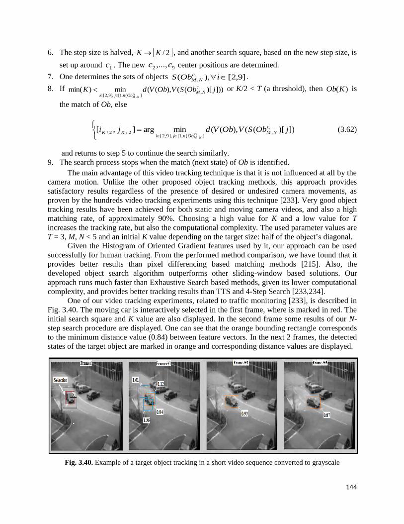
144
6. The step size is halved, 2/KK , and another search square, based on the new step size, is
set up around 1c . The new 92 ,...,cc center positions are determined.
7. One determines the sets of objects ]9,2[),( , iObS ic
NM.
8. If ])))[((),((min)min( ,](,1[],9,2[ ,
jObSVObVdK i
icNM
c
NMObnji
or K/2 < T (a threshold), then )(KOb is
the match of Ob, else
]))[((),((minarg],[ ,](,1[],9,2[
2/2/,
jObSVObVdji i
icNM
c
NMObnji
KK (3.62)
and returns to step 5 to continue the search similarly.
9. The search process stops when the match (next state) of Ob is identified.
The main advantage of this video tracking technique is that it is not influenced at all by the
camera motion. Unlike the other proposed object tracking methods, this approach provides
satisfactory results regardless of the presence of desired or undesired camera movements, as
proven by the hundreds video tracking experiments using this technique [233]. Very good object
tracking results have been achieved for both static and moving camera videos, and also a high
matching rate, of approximately 90%. Choosing a high value for K and a low value for T
increases the tracking rate, but also the computational complexity. The used parameter values are
T = 3, M, N < 5 and an initial K value depending on the target size: half of the object’s diagonal.
Given the Histogram of Oriented Gradient features used by it, our approach can be used
successfully for human tracking. From the performed method comparison, we have found that it
provides better results than pixel differencing based matching methods [215]. Also, the
developed object search algorithm outperforms other sliding-window based solutions. Our
approach runs much faster than Exhaustive Search based methods, given its lower computational
complexity, and provides better tracking results than TTS and 4-Step Search [233,234].
One of our video tracking experiments, related to traffic monitoring [233], is described in
Fig. 3.40. The moving car is interactively selected in the first frame, where is marked in red. The
initial search square and K value are also displayed. In the second frame some results of our N-
step search procedure are displayed. One can see that the orange bounding rectangle corresponds
to the minimum distance value (0.84) between feature vectors. In the next 2 frames, the detected
states of the target object are marked in orange and corresponding distance values are displayed.
Fig. 3.40. Example of a target object tracking in a short video sequence converted to grayscale
145
3.7. Conclusions
In this chapter we have described the most important results of our research conducted in
the last years in the computer vision domain. These results were disseminated in 2 books, 15
articles published in recognized international journals and 20 articles published in the volumes of
international scientific events. We brought major contributions in the next computer vision
fields: image and video segmentation, image reconstruction, image and object recognition,
content-based image indexing and retrieval, object detection and tracking.
The image segmentation task was treated by proposing original region-based and contour-
based approaches. Our automatic region-based segmentation techniques, which use various
moment-based pixel feature vectors and the automatic clustering algorithms developed by us,
provide very good results and execute quite fast. They represent better solutions than many other
state of the art segmentation methods because of their automatic character that is an important
advantage. The contour-based segmentation method developed by us represents an effective PDE
variational level-set based technique that improves the influential Chan-Vese level-set model. A
rigorous mathematical treatment of the proposed contour tracking PDE model was also provided.
We also constructed a novel automatic temporal video segmentation technique, based on a
robust Gabor filter-based feature extraction producing 3D frame feature vectors, and some
automatic no-threshold based frame clustering solutions. From our many experiments and
method comparisons we found that our approach outperforms the other state of the art cut
detection methods. It could be improved to work properly for other shot transitions, besides cuts.
Important results were also obtained in the image reconstruction domain. We developed a
PDE variational image inpainting approach characterized by a nonlinear elliptic diffusion Euler-
Lagrange equation, which restore properly the missing regions. The mathematical investigation
of this PDE model, performed by us, represents also an important contribution in this field.
We developed various image, video and object recognition techniques, which were
described in this chapter. Our main contributions in the image recognition area are the automatic
recognition models computing moment-based, LAB color based and 2D Gabor filter based
feature vectors that are next clustered by our unsupervised classification methods. The most
important contribution in the object recognition domain is our automatic moment-based shape
recognition technique, followed by a content-based analysis in the object recognition process.
Because of their automatic character, our recognition models are much more effective than other
existing techniques and more useful for content-based image indexing and retrieval, which is
another domain successfully approached by us. We proposed effective content-based feature
vector indexing solutions, developing both SAM-based indexing structures and cluster-based
image indexing models. Consequently, the corresponding CBIR techniques were obtained. We
developed an original cluster-based retrieval system that extracts relevant images and objects
from a database by using the indexes created through our automatic feature vector clustering
algorithms. We also constructed relevance-feedback based CBIR schemes that perform effective
K-NN searches at each step by using the tree-based SAM indexing structures.
Some significant detection and tracking results were also provided. Original object class
detection models, performing skin, face and human cell detection, were developed by us. The
temporal differencing-based multi moving object detection method is another major contribution
in this field. Novel object-matching based tracking approaches, using correlation-based, Gabor
filter-based and HOG-based features, were also proposed. Our pedestrian tracking models and
the motion-insensitive N-SS based tracking technique represent important contributions as well.

146
(ii) Professional, scientific and academic career evolvement
and development plans
In the main part of this thesis, b(i), there were presented the most important scientific
achievements of my research activity conducted in the period 2005-2014. In this second part,
b(ii), my professional, scientific and academic career evolvement and development plans are
outlined.
I began the research in image processing, biometrics and computer vision areas before
2005 and intend to continue it in the future. Several important results were obtained in the
respective areas before being awarded the PhD degree, some of them being already mentioned in
this thesis. Thus, in the image pre-processing field, we developed an application of the fractional
step algorithm for computing the Riccati equation’s solutions to image denoising and restoration
[235]. An effective restoration model for blurred and noisy images is provided in [235]. A
numerical approximation of the Riccati equation via fractional steps method, which can be also
applied to image filtering, is described in [236].
In the biometrics domain we modeled some person authentication techniques based on
voice and fingerprints. Our speaker recognition models using auto-regressive (AR) coefficient
based feature vectors classified using MLP, RBF [59] or various ART classifiers [60] were
mentioned in section 2.1. Also, some pattern-based fingerprint recognition techniques using 2D
Gabor filters, Wavelet Transforms and a combination of the two were proposed in [97]. Bimodal
biometric solutions based on voice and fingerprints were also considered. Some important results
were also achieved in the computer vision field. A moment-based image segmentation technique
developed in 2003 was shortly discussed in 3.1.1 [125]. An image object detection method using
the segmentation results obtained in [125] was proposed in [126]. Also, some image object
recognition and interpretation techniques are provided in that paper [126]. Another computer
vision system for image object recognition was proposed in 2004 [170].
Obviously, our research in these domains has intensified considerably following the PhD
award. We have tried to unify the research in these scientific fields, which are strongly related
anyway. So, the biometrics and computer vision represent the major domains of interest, while
image preprocessing and machine learning have been viewed as important helping domains for
them. So, the mathematical models for image processing and machine learning presented in first
chapter have the role to facilitate the biometrics and computer vision tasks. It is obvious that our
feature vector classification models are required by the recognition tasks of the two major
domains, while the images enhanced by pre-processing operations facilitate considerably any
image analysis process from the biometrics or computer vision domain. This relationship
between these research areas is also expressed in thesis title, which says that image processing
and analysis methods, and also the signal analysis used in voice recognition, are applied in the
two major fields.
As a unifying aspect, we have approached subdomains that could be part of more than one
domain. Since computer vision represents an extremely vast scientific domain that is closely
related to a lot of signal processing based research fields, it has significant overlaps with the
other three approached domains. For this reason some of our techniques described here can be
considered as belonging to two domains, instead of one. For example, some may consider the
clustering technologies of machine learning as part of computer vision, the image reconstruction
field could be also considered as an image pre-processing subdomain, some biometric

147
authentication processes described here, such as face recognition, represent also object
recognition tasks related to computer vision, while some of our computer vision tasks
representing object detection procedures, like face detection that is viewed as the first step of
face recognition, could also be included in biometrics.
Another important unifying element brought by us is the presence of mathematical models
in all the approached fields. Thus, PDE models are introduced to solve all our image processing
tasks, some PDE models are used in the biometric authentication domain (see our eigenimage-
based approach) and other PDE-based approaches are used in some computer vision subdomains,
such as image inpainting and contour tracking. Some mathematical models, although not PDE-
based, are used also by the proposed classification algorithms and their metrics. Strong
mathematical treatments are provided in all cases involving these models, proving the superiority
of partial differential equation based solutions to other approaches.
Our future research will focus on further improving these PDE models and developing
new PDE-based solutions for the tasks of the considered domains. As previously mentioned, the
main research directions of our future activity will remain essentially the same, but new
subdomains of image pre-processing, biometrics and computer vision can be approached. Let us
present now our future research plans in each of these fields.
So, I intend to develop new PDE-based techniques for image denoising and restoration and
to obtain improved versions of our existing models. For example, the image denoising technique
using hyperbolic second-order equations proposed in [5] can be further transformed into a more
sophisticated nonlinear filter, as already mentioned in 1.1. We will derive novel and effective
nonlinear PDE hyperbolic models from it, such as that given by (1.6), to achieve better image
filtering solutions. Another application of our hyperbolic model is a filtering technique that
extracts the coherent and incoherent components of a forced turbulent flow and to identify
coherent vortices [7].
The nonlinear anisotropic diffusion based image denoising and restoration techniques
described in 1.2 will also be improved. Thus, we are investigating successfully new edge-
stopping functions for our PDE models. Novel anisotropic diffusion schemes, like (1.19), will
also be modeled. Mathematical treatment of well-posedness, stability and consistency will be
performed for each of them. More effective discretization schemes will be also considered for
these PDE models, rigorous mathematical demonstrations of their convergence being provided.
The image noise removal approach based on diffusion porous media flow presented in
1.2.2 could also be modified. Thus, we will consider the following equation:
),0(in ,0),0(
,),0(in ,0),(
x
uxt
u
(1)
where will be a carefully chosen maximal monotone function. A robust mathematical
investigation of this nonlinear diffusion equation will be performed. We will try to demonstrate
that equation (1) has a unique strong solution in certain conditions. The numerical approximation
of this PDE will be performed using an implicit finite difference scheme. A stochastic variant of
this PDE model will also be studied. Thus, the stochastic equation udWuxt
u
),( may
be considered.

148
We also intend to improve our fourth-order diffusion-based image denoising approaches
[24], which are inspired by the influential You-Kaveh isotropic scheme [237], by modeling new
diffusivity functions. Also, we will develop nonlinear fourth-order anisotropic diffusion models
that outperform the Y-K algorithm and other state-of-the-art 4th-order PDEs, providing much
better despeckling and deblurring results. They will outperform also the second-order PDE
models, removing more successfully the staircase effect. These novel restoration solutions could
be achieved by mixing nonlinear 2nd-order and 4th-order diffusions. Such a combined 4th –order
PDE model has just been disseminated in an accepted article [238], and more denoising schemes
of that type will be investigated as part of our future research.
Our future research in image enhancement domain will also focus on modeling novel
variational schemes for image restoration. The PDE variational techniques described in section
1.3 can be further modified to obtain improved versions. New variants of the regularizer
function, which produce a better smoothing effect while preserving the image edges and
reducing the staircasing effect, will be proposed. Thus, we will investigate a modified version of
the variational PDE model presented in 1.3.2, which is based on the minimization of a convex
energy functional of gradient under minimal growth conditions [28]. A new image denoising
solution would be based on the following minimization problem:
,)(;2
1)(min 1,12
0
Wudxuuu
(2)
where ,: R is chosen as a convex lower semicontinuous function such that
rfor
rforg
,
),()(
0
(3)
where )()( 1
0 RCg . In this case, the corresponding elliptic equation has the following form:
0)( 0 uu(u)divu) div(g(
(4)
where (u) is the normal cone to 2121 ,, ; uuuauuu . This is an elliptic variational
inequality. This new denoising procedure refers to situation where one imposes a magnitude
constraint on the gradient of intensity that is a constant on variation of luminosity of the image.
In the biometrics domain our future research activity will focus on developing new person
authentication strategies based on the same identifiers (voice, face and fingerprints) and also
considering biometric recognition techniques based on new identifiers. So, we are going to
continue the research in the voice recognition area, paying particular attention to the text-
independent speaker recognition subdomain, where we have achieved considerably weaker
results. A MFCC-based speech signal analysis could be performed in the feature extraction stage,
but we will also investigate other voice feature extraction solutions, like those using linear
predictive cepstral coefficients (LPCCs) [239], for example. In the feature vector classification
stage, Vector Quantization (VQ) [63] or Gaussian Mixture Models (GMM) [64] can be applied.
New face recognition solutions will also be explored. So, I consider proposing some facial
recognition approaches based on tools that have been less utilized in our research, such as
149
Independent Component Analysis (ICA), Linear Discriminant Analysis (LDA) and Local Non-
negative Matrix Factorization (LNMF) [240].
In the fingerprint authentication domain we aim to extend the conventional recognition
from a supervised to an unsupervised framework. The unsupervised fingerprint recognition field
has been increasingly investigated in the last years [241]. We consider developing some
unsupervised fingerprint recognition techniques that outperform the existing approaches, our
technologies being endowed with an automatic character. The planned methods use both
minutia-based and pattern-based feature vectors. Our automatic clustering algorithms will be
applied to the fingerprint feature vectors, eventually using some special similarity metrics in the
minutia-based case.
As previously mentioned, our biometrics related research will also focus on a fourth
biometric identifier that is the human iris [242]. Our research in the iris recognition domain is
still in the early stage, a few results being achieved and disseminated [54,117]. An automatic
unsupervised iris recognition approach that classifies LAB color-based feature vectors by using a
hierarchical agglomerative clustering algorithm is proposed in [54]. A supervised iris-based
authentication model using other LAB color features and a K-NN classifier is provided by us in a
very recent paper [117]. Although the color analysis in LAB colorspace provides us encouraging
iris featuring results and we will continue the research in this area by improving the color-based
feature vectors, we are going to investigate other iris feature extraction solutions, too. Thus, the
future recognition approaches will take into consideration the iris texture information. Some
robust texture analysis based iris feature extraction solutions using two-dimensional Gabor filters
and Discrete Wavelet transforms will be constructed as part of our research. Next, we will try to
combine the color-based and texture-based features to obtain more powerful iris feature vectors
and consequently, much better recognition results.
New multimodal biometric recognition solutions will also be considered in the future. So,
adding the new biometric that is iris to our existing unimodal and multimodal biometric systems
based on various combinations of voice, face and fingerprints [53,59,60,91,97,113,116] would
improve considerably the authentication results. Also, some improved multi-method biometric
systems will be obtained by adding new voice, face, fingerprint and iris recognition techniques to
the existing models. As mentioned in 2.5, we will also try new biometric information fusion
solutions. Thus, we consider performing the fusion at lower levels than the decision level or even
the classification level.
My research activity in the computer vision domain will continue in the described
subdomains, but new computer vision areas will be also approached. Also, we intend to solve
more computer vision tasks by using the PDE models. We will consider new region-based and
contour-based image segmentation solutions. So, novel pixel clustering based segmentation
techniques can be obtained by using other feature extraction processes instead of the moment-
based analysis used in 3.1.1. The feature vector characterizing the neighborhood of a pixel can be
also modeled using other well-known image analysis tools, such as the 2D Gabor filters and
DWT-2D. Also, we will further investigate the level-set based segmentation domain [136],
trying to achieve new contour tracking-based image segmentation solutions.
We could search for some better featuring approaches in the video segmentation case, too,
but our main challenge in this case is to develop some temporal segmentation algorithms that
work properly not only for hard cuts, but also for other types of shot transitions. So, we will try
to improve the automatic video shot detection technique described in 3.2.2 [139], so it works
properly for soft cuts, like fades or dissolves, or some digital effects.

150
Image reconstruction will remain an important focus of my future computer vision
research. I consider developing more PDE-based inpainting techniques improving the well-
known TV inpainting model and the variational reconstruction model proposed in [134]. So,
novel variational inpainting models can be obtained from (3.28) if new proper edge-stoppping
functions are determined. Also, more effective variational reconstruction solutions will be
achieved by adapting the nonlinear fourth-order diffusion-based models to inpainting:
duuuuu
2
0
2 112
minarg* (5)
where function must be properly selected. Models combining 2nd and 4th order PDEs may be
also adapted for inpainting. Another idea is to construct an inpainting model based on the Cahn-
Hilliard equation [243]. So, we will investigate the PDE:
,,,0
,),0(in ,
0
32
yxuyxu
Tuuut
u
, (6)
corresponding to a variational model based on next minimization:
)(2
0 uEdxdyuuMinu
(7)
where
dxdyuuuE 1)( 22
We also intend to obtain new results in the image and object recognition field. A novel
image recognition approach would imply either a new image featuring solution or a new feature
vector classification method. New and possibly improved content-based feature vectors will be
modeled by performing new color and texture analysis procedures. Thus, we will continue to
investigate the LAB color-based image analysis, trying to achieve better color feature vectors.
Also, new texture-based image analysis operations based on 2D Gabor filters, 2D-DWT and
Fourier descriptors will be performed. Novel image similarity metrics will be considered for
these feature vectors. We will also perform new research in the machine learning domain,
focusing mainly on identifying automatic unsupervised classification solutions. Obviously, any
new feature vector classification approach would produce not only novel image recognition
solutions, but also many new biometric authentication methods. Novel object recognition models
will also be considered, new shape descriptors being modeled for this purpose. High-level image
analysis will also be a focus of my research, new object interpretation models being investigated.
Our future research in content-based image indexing and retrieval domain is closely
related to content-based image/video and object recognition research. We intend to implement
new versions of the relevance-feedback based CBIR system represented in Fig. 3.20, by
considering new SAM-based high-dimensional data indexing solutions. Thus, various search
tree-based structures, such as VP-tree, M-tree or MVP-tree, will be used for the new modeled
content-based image feature vectors.
151
Novel object detection and tracking solution will be developed during our future research,
too. As previously mentioned, the PDE level-set based contour tracking techniques for image
segmentation and object detection in static images will be further investigated. Other object
detection tools, such as the point detectors, various Hough Transforms or boosting procedures,
will be applied. New object-class detection tasks will be also performed. I am going to continue
the research in the face detection domain, providing other solutions to this task. For example, the
proposed face detection model using skin identification results can be further modified [168].
Thus, the face candidates are determined using the same conditions given in (3.45). These
candidates represent filled connected components, so their original (unfilled) versions are then
analyzed. Those of them characterized by holes that could represent essential facial features such
as eyes, eyebrows, nose and mouth, are labeled as faces. Some geometric approaches can be used
to identify these individual face characteristics.
Human detection in static images will constitute another important goal of our computer
vision research. An idea is to extend the skin-based solution used in the cases of faces for
detecting entire human bodies. Obviously, the detected skin regions representing face, neck,
arms, hands, legs and feet could determine the location of a person. The task becomes more
difficult if some of these body parts are covered by clothes. Another solution is to apply a
technique that is similar to the SVM-based approach proposed for cell detection [210]. Our
sliding-window based image scanning algorithm, or an improved version of it, and the HOG-
based feature extraction will be used successfully for pedestrian detection, if a proper training
set, containing human and non-human image objects, is constructed for SVM. Also, replacing
the HOG features with other featuring solutions in this detection process will be considered. We
also intend to improve the proposed multiple moving object detection technique [219], so that to
become less influenced by the video camera motion. Novel object tracking solutions will be also
developed. We consider using Kalman filtering with some point-based features, like SIFT.
Introducing the PDE models in our object detection and tracking research represents another
future goal. Thus, a PDE-based video motion estimation that would be very useful to the tracking
process will be performed. Our estimation approach will compute efficiently the optical flow
from the video sequences [244], by using a new PDE variational model. A energy functional to
be minimized will be constructed and solving the minimization problem will require 2 Euler-
Lagrange equations.
New computer vision subdomains will be considered, as part of our future research. One of
them is the image registration that involves spatially registering the target image(s) to align with
the reference image [245]. Since image similarities are broadly used for image registration, our
image similarity metrics can be applied successfully to this domain. Also, some PDE-based
registration techniques are planned [246]. Similar to optic flow case, one estimates a realistic
displacement (deformation) field mapping corresponding pixels in the template image to the
source image, in registration case. So, an effective PDE variational image registration model can
be derived from the variational optical flow estimation solutions.
I have also some serious professional and academic career evolvement and development
plans. My actual academic position is Senior Researcher I at Institute of Computer Science of the
Romanian Academy. Following this abilitation process, I will obtain also the official right of
doctoral supervision. So, an important objective of my future professional activity is to form a
new generation of well-prepared researchers in my domains of interest. For this purpose I intend
to recruit and supervise PhD students that have passion for this research and willingness to work
hard in the research collectives coordinated by me.

152
Building and managing these effective research teams represents another essential
objective. Given my high research position, I have a rich experience as a team leader. Since 2004
I have been coordinating a research collective at my institute, whose activity is related to speech,
image and video processing and analysis. In the period following my PhD award, our research
team has achieved important results in these scientific fields. Thus, 22 of my papers published
since 2005 in these domains have some of the members of my research team as co-authors. Also,
in this period our research collective has elaborated 20 scientific reports under my supervision,
disseminating image processing, biometrics and computer vision results. I intend to strengthen
and also enlarge my research team in the future, by co-opting preferably young researchers and
PhD students. Since my future doctoral students will follow their PhD program at Institute of
Computer Science, they could also participate at our research projects, so I will try to enlarge our
team by including them. Besides coordinating this collective at the institute, I am going to
organize research teams related to various projects. Since 2005 I have coordinated several
research directions, related to biometrics, PDE models and computer vision, in scientific projects
(grants) on the basis of contract. In the future I intend to build some strong and larger research
teams with whom to win more grant competitions as project director. My future PhD students
will also be included in these project-related collectives.
Another objective of my academic career development plan consists of establishing some
important collaborative relationships with other institutions and researchers from our country or
abroad. In the last years I have established several external collaborations, by performing
research and teaching activities at three important foreign universities. So, in May 2012 I
activated as visiting academic at Department of Automatic Control and Systems Engineering of
the University of Sheffield, United Kingdom, working with a british research team in a video
analysis project. In April 2013 I worked for one month as a visiting professor at the University of
Bologna, Italy. During that visit I collaborated with professor Angelo Favini, from Department
of Mathematics of the university, in the PDE-based image processing domain. The results of our
research collaboration were disseminated in a paper published in an ISI journal [16], and
included in my most relevant 10 papers. In 2014 I won a DAAD fellowship for university
professors and senior researchers with a project in PDE-based image restoration field. My
DAAD project, entitled VANDIRES, was conducted at the Department of Mathematics of the
Bielefeld University, Germany, in collaboration with a research team led by the professor
Michael Roeckner. Last year I also won a GNAMPA fellowship for visiting professors, with
another PDE-based computer vision project, which will allow me to work again at Bologna
University later this year and to continue the collaboration with its Department of Mathematics.
A collaboration with Faculty of Bioengineering of University of Medicine and Pharmacy from
Iaşi is also underway. I will continue these collaborations in the future while trying to establish
more external cooperations. I believe that all these collaborations will result not only in new
published papers and academic exchange visits, but also in strong international research
collectives capable to win and conduct bilateral and multinational projects based on contract.
The final main objective is to perform some teaching activity, besides research, in the
mentioned areas. Altough my scientific activity has consisted mainly of research, I have also
some teaching experience. I activated as visiting professor at Bologna University and Bielefeld
University, giving numerous talks at those institutions. Also I have delivered many lectures to
the students of the Faculty of Bioengineering of University of Medicine and Pharmacy, Iaşi. So, I
would like to continue to transmit my knowledge to young people and I strongly believe that
teaching and working with students will be also very helpful to my research career.
153
(iii) References
[1] F. Guichard, L. Moisan, J. M. Morel, A review of P.D.E. models in image processing and image
analysis, Journal de Physique, Vol. 4, pp. 137–154, 2001.
[2] A. K. Jain, Fundamentals of Digital Image Processing, Prentice Hall, NJ, USA, 1989.
[3] R. Gonzales, R.Woods, Digital Image Processing, Prentice Hall, New York, NY, USA, 2nd edition,
2001.
[4] H. E. Ning, L. U. A. Ke, A Non Local Feature-Preserving Strategy for Image Denoising, Chinese
Journal of Electronics, Vol. 21, No. 4, 2012.
[5] T. Barbu. Novel linear image denoising approach based on a modified Gaussian filter kernel,
Numerical Functional Analysis and Optimization, 33 (11), pp. 1269-1279, publisher Taylor & Francis
Group, LLC, 2012.
[6] V. Barbu, Partial Diferential Equations and Boundary Value Problems, Kluwer Academic Publishers,
Dordrecht, 1998.
[7] T. Nabi, W. A. Kareem, S. Izawa, Y. Fukumishi, Extraction of coherent vortices from homogeneous
turbulence using curvelets and total variation filtering methods, Computers and Fluids, Vol. 57, pp.
76-86 2012.
[8] J. Weickert, Anisotropic Diffusion in Image Processing, European Consortium for Mathematics in
Industry, B. G. Teubner, Stuttgart, Germany, 1998.
[9] P. Perona, J. Malik, Scale-space and edge detection using anisotropic diffusion, Proceedings of IEEE
Computer Society Workshop on Computer Vision, 16–22, nov. 1987.
[10] S. Esedoglu, An analysis of the Perona-Malik scheme, Comm. Pure Appl. Math., 54, pp. 1442-1487,
2001.
[11] T. F. Chan, C. K. Wong, Total variation blind deconvolution, IEEE Transactions on Image
Processing, 7, pp. 370–375, 1998.
[12] P. Charbonnier, L. Blanc-Feraud, G. Aubert, M. Barlaud, Two deterministic half-quadratic
regularization algorithms for computed imaging, Proc. IEEE International Conf. on Image Processing,
vol. 2, pp. 168–172, Austin, TX, IEEE Comp. Society Press, 1994.
[13] M. Black, G. Shapiro, D. Marimont, D. Heeger, Robust anisotropic diffusion, IEEE Trans. Image
Processing, 7, 3, pp. 421-432, 1998.
[14] F. Voci, S. Eiho, N. Sugimoto, H. Sekiguchi, Estimating the gradient threshold in the Perona–Malik
equation, IEEE Signal Processing Magazine, 21 (3), pp. 39-46, 2004.
[15] T. Barbu, Robust anisotropic diffusion scheme for image noise removal, Procedia Computer Science
(Proc. of 18th International Conf. in Knowledge Based and Intelligent Information & Engineering
Systems, KES 2014, Sept. 15-17, Gdynia, Poland), published by Elsevier, Vol. 35, pp. 522-530, 2014.
[16] T. Barbu, A. Favini, Rigorous mathematical investigation of a nonlinear anisotropic diffusion-
based image restoration model, Electronic Journal of Differential Equations, Vol. 2014, No. 129,
pp. 1-9, 2014.
[17] S. L. Keeling, R. Stollberger, Nonlinear anisotropic diffusion filtering for multiscale edge
enhancement, Inverse Problems, vol 18, pp. 175-190, 2002.
[18] T. Barbu, Variational image denoising approach with diffusion porous media flow, Abstract and
Applied Analysis, Volume 2013, Article ID 856876, 8 pages, Hindawi Publishing Corporation, 2013,
DOI: http://dx.doi.org/10.1155/2013/856876.
[19] J. Kačur, K. Mikula, Slow and fast diffusion effects in image processing, Computing and
Visualization in Science, vol. 13, no. 4, pp. 185–195, 2001.
[20] A. Buades, B. Coll, J-M. Morel, The staircasing effect in neighborhood filters and its solution, IEEE
Transactions on Image Processing 15, 6, pp. 1499-1505, 2006.
[21] M. Mansourpour, M. A. Rajabi, J. R. Blais, Effects and performance of speckle noise reduction
filters on active radars and SAR images, Proceedings of ISPRS 2006, Ankara, Turkey, Feb. 14-16,
XXXVI-1/W41 2006.

154
[22] S. Sudha, G. R. Suresh, R. Sukanesh, Speckle Noise Reduction in Ultrasound Images by Wavelet
Thresholding based on Weighted Variance, International Journal of Computer Theory and
Engineering, Vol. 1, No. 1, pp. 1793-8201, April 2009.
[23] N. P. Anil, S. Natarajan, A New Technique for Image Denoising Using Fourth Order PDE and
Wiener Filter, International Journal of Applied Engineering Research, Volume 5, Issue 3, 2010.
[24] T. Barbu, A PDE based Model for Sonar Image and Video Denoising, Analele Stiintifice ale
Universitatii Ovidius, Constanta, Seria Matematică, Vol. 19, Fasc. 3, pp. 51-58, 2011.
[25] L. Rudin, S. Osher, E. Fatemi, Nonlinear total variation based noise removal algorithms, Physica D:
Nonlinear Phenomena, 60.1, pp. 259-268, 1992.
[26] T. Chan, J. Shen, L. Vese, Variational PDE Models in Image Processing, Notices of the AMS, Vol.
50, No. 1, 2003.
[27] T. Barbu, A Novel Variational PDE Technique for Image Denoising, Lecture Notes in Computer
Science (Proc. of the 20th International Conference on Neural Information Processing, ICONIP 2013,
part III, Daegu, Korea, Nov. 3-7, 2013), Vol. 8228, pp. 501-508, Springer-Verlag Berlin Heidelberg,
M. Lee et al. (Eds.), 2013.
[28] T. Barbu, V. Barbu, V. Biga, D. Coca, A PDE variational approach to image denoising and
restoration, Nonlinear Analysis: Real World Applications, Vol. 10, Issue 3, pp. 1351-1361, June 2009.
[29] K. Popuri, Introduction to Variational Methods in Imaging, CVR 2010 Tutorial Talk, May 2010.
[30] C. Fox, An introduction to the calculus of variations, Courier Dover Publications, 1987.
[31] T. Barbu, Speech-dependent voice recognition system using a nonlinear metric, International
Journal of Applied Mathematics, Volume 18, No. 4, pp. 501-514, 2005.
[32] L. Alboaie, T. Barbu, An Automatic User Recognition Approach within a Reputation System Using
a Nonlinear Hausdorff Derived Metric, Numerical Functional Analysis and Optimization, published by
Taylor & Francis, Vol. 29, Issue 11 & 12, pp. 1240 – 1251, Nov. 2008.
[33] T. Barbu, Modelling Multimedia Information Systems (in Romanian), edited by Romanian Academy
Publishing House, Bucharest, 225 pages, 2006.
[34] J. Henrikson, Completeness and Total Boundedness of the Hausdorff Metric, The MIT
Undergraduate Journal of Mathematics, Volume 1, pp. 69-80, 1999.
[35] J. von Neumann, Zur Theorie der Gesellschaftsspiele, Mathematische Annalen, 100, pp. 295-320,
1928.
[36] T. Barbu, Comparing Various Voice Recognition Techniques, From Speech Processing to Spoken
Language Technology (Proc. of 5th International Conference on Speech Technology and Human-
Computer Dialogue, SPED’09), eds. Academy Publishing House, pp. 33-42, Constanta, Romania,
June 18-21, 2009.
[37] T. Barbu, Unsupervised SIFT-based Face Recognition Using an Automatic Hierarchical
Agglomerative Clustering Solution, Procedia Computer Science (Proceedings of 17th International
Conference in Knowledge Based and Intelligent Information and Engineering Systems, KES 2013,
Sept. 9-11, Kitakyushu, Japan), Vol. 22, pp. 385-394, published by Elsevier, 2013.
[38] T. Barbu, Fingerprint Matching Approach Using a Novel Metric, U.P.B. Scientific Bulletin,
Series A, Issue 2, Vol. 73, pp. 119-128, 2011.
[39] T. Barbu, An Automatic Unsupervised Pattern Recognition Approach, Proceedings of the Romanian
Academy, Series A: Mathematics, Physics, Technical Sciences, Information Science, Vol. 7, No. 1, pp.
73-78, January-April 2006.
[40] T. Barbu, Automatic Unsupervised Shape Recognition Technique using Moment Invariants,
Proceedings of the 15th International Conference on System Theory, Control and Computing, ICSTCC
2011, pp. 93-96, Sinaia, Romania, 14-16 Oct. 2011.
[41] T. Barbu, Unsupervised Speaker Recognition Approach using an Automatic Clustering Algorithm,
Proceedings of the 7th Conference on Speech Technology and Human-Computer Dialogue, SpeD 2013,
Cluj-Napoca, Romania, pp. 215-220, 16-19 October 2013.

155
[42] T. Barbu, Automatic Texture-based Image Segmentation Technique, Proceedings of The 6th
European Conference on Intelligent Systems and Technologies, ECIT’10, October 7-9, Iaşi, Romania,
2010.
[43] C-T. Chang, J. Z. C. Lai, M-D. Jeng, A Fuzzy K-means Clustering Algorithm Using Cluster Center
Displacement, Journal of Information Science And Engineering, 27, pp. 995-1009, 2011.
[44] I. Lapidot, H. Guterman, A. Cohen, Unsupervised Speaker Recognition Based on Competition
Between Self-Organizing Maps, IEEE Transactions on Neural Networks, vol. 13, no. 4, July 2002.
[45] T. Kanungo, D. M. Mount, N. S. Netanyahu, C. D. Piatko, R. Silverman, A. Y. Wu, An Efficient K-
Means Clustering Algorithm: Analysis and Implementation, IEEE Trans. on Pattern Analysis and
Machine Intelligence, Vol. 24, Number 7, pp. 881-892, 2002.
[46] J. Dunn, Well separated clusters and optimal fuzzy partitions, Journal of Cybernetics, Vol. 4, pp. 95-
104, 1974.
[47] D. L. Davies, D. W. Bouldin, A cluster separation measure, IEEE Transactions on Pattern Analysis
and Machine Intelligence, Vol. 1 (4), pp. 224-227, 2000.
[48] T. Barbu, M. Costin, A. Ciobanu, An Unsupervised Content-based Image Recognition Technique,
Springer-Verlag - Series: Studies in Computational Intelligence: New Concepts and Applications in
Soft Computing, Vol. 417, pp. 157-164, Berlin, Eds. V. E. Balas, A. V. Koczy, J. Fodor, 2013.
[49] A. K. Jain, P. Flynn, A. Ross, Handbook of Biometrics, Springer, 2007.
[50] H. F. Tipton, M. Krause, Information Security Management Handbook, Sixth Edition, published by
CRC Press, 3280 pages, May 14, 2007.
[51] M. G. Milone, Biometric surveillance: searching for identity, Business Lawyer, Nov. 1, 2001.
[52] A. K. Jain, R. Bolle, S. Pankanti, Biometrics: Personal Identification in Networked Society, Kluwer
Academic Publications, 1999.
[53] T. Barbu, Biometric Authentication Techniques (in Romanian), edited by Romanian Academy
Publishing House, Bucharest, 110 pages, 2012.
[54] A. Ciobanu, P. Radu, T. Barbu, M. Costin, S. I. Bejinariu, A Novel Iris Clustering Approach Using
LAB Color Features, Proceedings of the 4th International Symposium on Electrical and Electronics
Engineering, Galati, Romania, Oct. 11-13, 2013.
[55] R. A. Cole, J. Mariani, H. Uszkoreit, A. Zaenen, V. Zue, Survey of the State of the Art in Human
Language Technology, Cambridge University Press, 1997.
[56] D. A. Reynolds, R. C. Rose, Robust text-independent speaker identification using Gaussian mixture
speaker models, IEEE Trans. Speech Audio Processing, vol. 3, no. 1, pp. 72-83, 1995.
[57] T. Barbu, A supervised text-independent speaker recognition approach, International Journal of
Computer, Information, Systems and Control Engineering, Vol. 1, No. 9, 2007.
[58] T. F. Zheng, G. Zhang, Z. Song, Comparison of Different Implementations of MFCC, Journal of
Computer Science and Technology, 16 (6), pp. 582-589, 2001.
[59] M. Costin, T. Barbu, A. Grichnik, Automatic Speaker Recognition Decision Tools, Fuzzy Systems
and Artificial Intelligence - Reports and Letters, Vol. 10, No. 3, pp. 167-181, 2004.
[60] T. Barbu, M. Costin, Comparing Various Automatic Speaker Recognition Approaches, Scientific
Bulletin of the Polytechnic University of Timisoara, Romania, Transactions on Electronics and
Communications, Tom (49) 63, Fasc. 1, pp. 291-296, 2004.
[61] Y. Zhang, Z-M. Tang, Y-P. Li, B. Qian, Ensemble Learning and Optimizing KNN Method for
Speaker Recognition, Proc. of 4th International Conference on Fuzzy Systems and Knowledge
Discovery, FSKD ‘07, Vol. 4, pp. 285-289, 24-27 Aug. 2007.
[62] W.M. Campbell, A SVM/HMM system for speaker recognition, Proc. ICASSP 2003, April 2003.
[63] F. Soong et. al., A vector quantization approach to speaker recognition, in Proc. IEEE ICASSP, pp.
387-390, 1985.
[64] L. Liu, J. He, On the use of orthogonal GMM in 385 speaker recognition, IEEE International
Conference on 386 Acoustic, Speech, and Signal Processing, ICASSP’99, vol. 2, pp. 845-849, 1999.
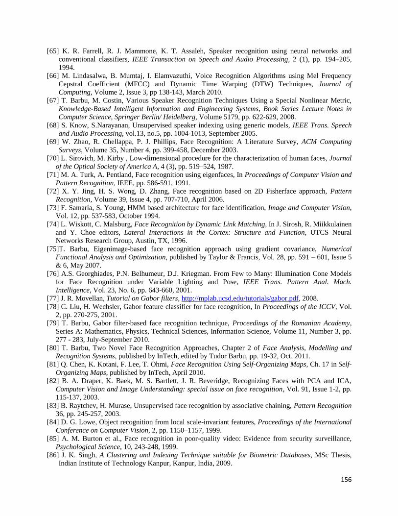
156
[65] K. R. Farrell, R. J. Mammone, K. T. Assaleh, Speaker recognition using neural networks and
conventional classifiers, IEEE Transaction on Speech and Audio Processing, 2 (1), pp. 194–205,
1994.
[66] M. Lindasalwa, B. Mumtaj, I. Elamvazuthi, Voice Recognition Algorithms using Mel Frequency
Cepstral Coefficient (MFCC) and Dynamic Time Warping (DTW) Techniques, Journal of
Computing, Volume 2, Issue 3, pp 138-143, March 2010.
[67] T. Barbu, M. Costin, Various Speaker Recognition Techniques Using a Special Nonlinear Metric,
Knowledge-Based Intelligent Information and Engineering Systems, Book Series Lecture Notes in
Computer Science, Springer Berlin/ Heidelberg, Volume 5179, pp. 622-629, 2008.
[68] S. Know, S.Narayanan, Unsupervised speaker indexing using generic models, IEEE Trans. Speech
and Audio Processing, vol.13, no.5, pp. 1004-1013, September 2005.
[69] W. Zhao, R. Chellappa, P. J. Phillips, Face Recognition: A Literature Survey, ACM Computing
Surveys, Volume 35, Number 4, pp. 399-458, December 2003.
[70] L. Sirovich, M. Kirby , Low-dimensional procedure for the characterization of human faces, Journal
of the Optical Society of America A, 4 (3), pp. 519–524, 1987.
[71] M. A. Turk, A. Pentland, Face recognition using eigenfaces, In Proceedings of Computer Vision and
Pattern Recognition, IEEE, pp. 586-591, 1991.
[72] X. Y. Jing, H. S. Wong, D. Zhang, Face recognition based on 2D Fisherface approach, Pattern
Recognition, Volume 39, Issue 4, pp. 707-710, April 2006.
[73] F. Samaria, S. Young, HMM based architecture for face identification, Image and Computer Vision,
Vol. 12, pp. 537-583, October 1994.
[74] L. Wiskott, C. Malsburg, Face Recognition by Dynamic Link Matching, In J. Sirosh, R. Miikkulainen
and Y. Choe editors, Lateral Interactions in the Cortex: Structure and Function, UTCS Neural
Networks Research Group, Austin, TX, 1996.
[75]T. Barbu, Eigenimage-based face recognition approach using gradient covariance, Numerical
Functional Analysis and Optimization, published by Taylor & Francis, Vol. 28, pp. 591 – 601, Issue 5
& 6, May 2007.
[76] A.S. Georghiades, P.N. Belhumeur, D.J. Kriegman. From Few to Many: Illumination Cone Models
for Face Recognition under Variable Lighting and Pose, IEEE Trans. Pattern Anal. Mach.
Intelligence, Vol. 23, No. 6, pp. 643-660, 2001.
[77] J. R. Movellan, Tutorial on Gabor filters, http://mplab.ucsd.edu/tutorials/gabor.pdf, 2008.
[78] C. Liu, H. Wechsler, Gabor feature classifier for face recognition, In Proceedings of the ICCV, Vol.
2, pp. 270-275, 2001.
[79] T. Barbu, Gabor filter-based face recognition technique, Proceedings of the Romanian Academy,
Series A: Mathematics, Physics, Technical Sciences, Information Science, Volume 11, Number 3, pp.
277 - 283, July-September 2010.
[80] T. Barbu, Two Novel Face Recognition Approaches, Chapter 2 of Face Analysis, Modelling and
Recognition Systems, published by InTech, edited by Tudor Barbu, pp. 19-32, Oct. 2011.
[81] Q. Chen, K. Kotani, F. Lee, T. Ohmi, Face Recognition Using Self-Organizing Maps, Ch. 17 in Self-
Organizing Maps, published by InTech, April 2010.
[82] B. A. Draper, K. Baek, M. S. Bartlett, J. R. Beveridge, Recognizing Faces with PCA and ICA,
Computer Vision and Image Understanding: special issue on face recognition, Vol. 91, Issue 1-2, pp.
115-137, 2003.
[83] B. Raytchev, H. Murase, Unsupervised face recognition by associative chaining, Pattern Recognition
36, pp. 245-257, 2003.
[84] D. G. Lowe, Object recognition from local scale-invariant features, Proceedings of the International
Conference on Computer Vision, 2, pp. 1150–1157, 1999.
[85] A. M. Burton et al., Face recognition in poor-quality video: Evidence from security surveillance,
Psychological Science, 10, 243-248, 1999.
[86] J. K. Singh, A Clustering and Indexing Technique suitable for Biometric Databases, MSc Thesis,
Indian Institute of Technology Kanpur, Kanpur, India, 2009.
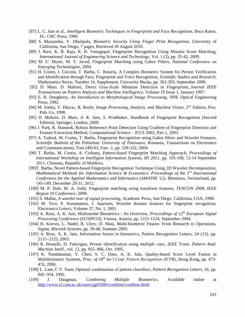
157
[87] L. C. Jain et al., Intelligent Biometric Techniques in Fingerprint and Face Recognition, Boca Raton,
FL: CRC Press, 1999.
[88] S. Mazumdar, V. Dhulipala, Biometric Security Using Finger Print Recognition, University of
California, San Diego, 7 pages, Retrieved 30 August 2010.
[89] J. Ravi, K. B. Raja, K. R. Venugopal, Fingerprint Recognition Using Minutia Score Matching,
International Journal of Engineering Science and Technology, Vol. 1 (2), pp. 35-42, 2009.
[90] M. U. Munir, M. Y. Javed, Fingerprint Matching using Gabor Filters, National Conference on
Emerging Technologies, 2004.
[91] H. Costin, I. Ciocoiu, T. Barbu, C. Rotariu, A Complex Biometric System for Person Verification
and Identification through Face, Fingerprint and Voice Recognition, Scientific Studies and Research,
Mathematics Series, Number 16, Supplement, University Bacău, pp. 361-393, September 2006.
[92] D. Maio, D. Maltoni, Direct Gray-Scale Minutiae Detection in Fingerprints, Journal IEEE
Transactions on Pattern Analysis and Machine Intelligence, Volume 19 Issue 1, January 1997.
[93] E. R. Dougherty, An Introduction to Morphological Image Processing, SPIE Optical Engineering
Press, 1992.
[94] M. Sonka, V. Hlavac, R. Boyle, Image Processing, Analysis, and Machine Vision, 2nd Edition, Pws.
Pub. Co, 1998.
[95] D. Maltoni, D. Maio, A. K. Jain, S. Prabhakar, Handbook of Fingerprint Recognition (Second
Edition), Springer, London, 2009.
[96] J. Park, K. Hanseok, Robust Reference Point Detection Using Gradient of Fingerprint Direction and
Feature Extraction Method, Computational Science – ICCS 2003, Part 1, 2003.
[97] A. Tudosă, M. Costin, T. Barbu, Fingerprint Recognition using Gabor filters and Wavelet Features,
Scientific Bulletin of the Politehnic University of Timisoara, Romania, Transactions on Electronics
and Communications, Tom (49) 63, Fasc. 1, pp. 328-332, 2004.
[98] T. Barbu, M. Costin, A. Ciobanu, Pattern-based Fingerprint Matching Approach, Proceedings of
International Workshop on Intelligent Information Systems, IIS 2011, pp. 105-108, 12-14 September
2011, Chisinau, Republic of Moldova.
[99]T. Barbu, Novel Pattern-based Fingerprint Recognition Technique Using 2D Wavelet Decomposition,
Mathematical Methods for Information Science & Economics: Proceedings of the 3rd International
Conference for the Applied Mathematics and Informatics (AMATHI '12), Montreux, Switzerland, pp.
145-149, December 29-31, 2012.
[100] M. P. Dale, M. A. Joshi, Fingerprint matching using transform features, TENCON 2008, IEEE
Region 10 Conference, 2008.
[101] S. Mallat, A wavelet tour of signal processing, Academic Press, San Diego, California, USA, 1998.
[102] M. Tico, P. Kuosmanen, J. Saarinen, Wavelet domain features for fingerprint recognition,
Electronics Letters, Volume 37, No. 1, 2001.
[103] A. Ross, A. K. Jain, Multimodal Biometrics : An Overview, Proceedings of 12th European Signal
Processing Conference (EUSIPCO), Vienna, Austria, pp. 1221-1224, September 2004.
[104] H. Korves, L. Nadel, B. Ulery, D. Masi, Multi-biometric Fusion: From Research to Operations,
Sigma, Mitretek Systems, pp. 39-48, Summer 2005.
[105] A. Ross, A. K. Jain, Information fusion in biometrics, Pattern Recognition Letters, 24 (13), pp.
2115–2125, 2003.
[106] R. Brunelli, D. Falavigna, Person identification using multiple cues, IEEE Trans. Pattern Anal.
Machine Intell., vol. 12, pp. 955–966, Oct. 1995.
[107] K. Nandakumar, Y. Chen, S. C. Dass, A. K. Jain, Quality-based Score Level Fusion in
Multibiometric Systems, Proc. of 18th Int’l Conf. Pattern Recognition (ICPR), Hong Kong, pp. 473-
476, 2006.
[108] L. Lam, C.Y. Suen, Optimal combination of pattern classifiers, Pattern Recognition Letters, 16, pp.
945–954, 1995.
[109] J. Daugman, Combining Multiple Biometrics, Available online at
http://www.cl.cam.ac.uk/users/jgd1000/combine/combine.html.
158
[110]L.Xu, A.Krzyzak, C. Suen, Methods of combining multiple classifiers and their applications to hand
writing recognition, IEEE Trans. on Systems, Man and Cybernetics, Vol. 22, no. 3, pp. 418–435,
1992.
[111] A. K. Jain, L. Hong, Y. Kulkarni, A multimodal biometric system using fingerprint, face and
speech, in Second International Conference on AVBPA, Washington D.C., USA, pp. 182–187, 1999.
[112] BioID, www.bioid.com.
[113] H. Costin, T. Barbu, C. Rotariu, C. Costin, A Biometric System for Person Verification and
Identification through Fingerprint and Voice Recognition, Proceedings of The 5th European
Conference on Intelligent Systems and Technologies, ECIT’08, Iaşi, Romania, July 10-12, 2008.
[114] L. Hong, A. Jain, Integrating faces and fingerprint for personal identification, IEEE Trans. Pattern
Analysis and Machine Intelligence 20 (12), pp. 1295–1307, 1998.
[115] H. Costin, I. Ciocoiu, T. Barbu, C. Rotariu, Through Biometric Card in Romania: Person
Identification by Face, Fingerprint and Voice Recognition, International Journal of Computer,
Information, Systems and Control Engineering, Vol. 2, No. 5, 2008.
[116] T. Barbu, M. Costin. A Human Person Recognition System using Face and Voice Biometrics,
Scientific Bulletin of the Politehnic University of Timisoara, Romania, Transactions on Electronics
and Communications, Tom (53) 67, Fasc. 2, pp. 5-10, 2008.
[117] A. Ciobanu, M. Luca, I. Păvăloi, T. Barbu, Iris Identification based on Optimized LAB Histograms
Applied to Iris Partitions, Bulletin of the Polytechnic Institute of Iasi, Automatic Control and
Computer Science Section, Tom LX (LXIV), Fasc. 3, pp. 37-48, published by "Gheorghe Asachi"
Technical University of Iaşi, 2014.
[118] L. G. Shapiro, G. C. Stockman, Computer Vision, Prentice Hall, 2001.
[119] R. Ohlander, K. Price, R. Reddy, Picture Segmentation Using a Recursive Region Splitting Method,
Computer Graphics and Image Processing, 8 (3), pp. 313–333, 1978.
[120] L. Barghout, J. Sheynin, Real-world scene perception and perceptual organization: Lessons from
Computer Vision, Journal of Vision, 13, 9, pp. 709-709, 2013.
[121] Z. Wu, R. Leahy, An optimal graph theoretic approach to data clustering: Theory and its application
to image segmentation, IEEE Transactions on Pattern Analysis and Machine Intelligence, Vol. 15,
No. 11, pp. 1101–1113, 1993.
[122] T. Lindeberg, M.-X. Li, Segmentation and classification of edges using minimum description
length approximation and complementary junction cues, Computer Vision and Image Understanding,
vol. 67, no. 1, pp. 88-98, 1997.
[123] S. Osher, N. Paragios, Geometric Level Set Methods in Imaging Vision and Graphics, Springer
Verlag, 2003
[124] M. Kass, A. Witkin, D. Terzopoulos, Snakes: Active contour models, International Journal of
Computer Vision, 1(4), pp. 321–331, 1987.
[125] T. Barbu, A Pattern Recognition Approach to Image Segmentation, Proceedings of the Romanian
Academy, Series A, Volume 4, Number 2, pp. 143-148, May-August 2003
[126] T. Barbu, Automatic Moment Based Texture Segmentation, International Journal of Computer,
Information Science and Engineering, Vol. 7, No. 12, pp. 813-818, 2013.
[127] M. Tuceryan, A. K. Jain, Texture Analysis. Handbook Pattern Recognition and Computer Vision.
Singapore: World Scientific, ch. 2, pp. 235–276, 1993.
[128] V. Levesque, Texture segmentation using Gabor filters, Center for Intelligent Machines Journal,
2000.
[129] M. N. Do, M. Vetterli, Wavelet-Based Texture Retrieval Using Generalized Gaussian Density and
Kullback-Leibler Distance, IEEE Transactions on Image Processing, 11:2, February 2002.
[130] B. Abraham, O. I. Camps, M. Sznaier, Dynamic Texture with Fourier Descriptors, Proceedings of
the 4th International Workshop on Texture Analysis and Synthesis, pp. 53-58, 2005.
[131] M. Tuceryan, A. K. Jain, Texture Segmentation Using Voronoi Polygons, IEEE Transactions on
Pattern Analysis and Machine Intelligence, PAMI-12, pp. 211-216, 1990.

159
[132] R. M. Haralick, K. Shanmugam, I. Dinstein, Textural features for image classification, IEEE
Transactions on Systems, Man, and Cybernetics, SMC - 3, pp. 610 – 621, 1973.
[133] N. Forcade, C. Le Guyader, C. Gout, Generalized fast marching method: applications to image
segmentation, Numerical Algorithms, 48 (1-3), pp. 189–211, July 2008.
[134] T. Barbu, Robust contour tracking model using a variational level-set algorithm, Numerical
Functional Analysis and Optimization, publisher Taylor & Francis Group, LLC, Vol. 35, Issue 3,
pp. 263-274, 2014.
[135] S. Osher, J. A. Sethian, Fronts propagating with curvature-dependent speed: Algorithms based on
Hamilton-Jacobi formulations, Journal of Computation Physics, 79, pp. 12–49, 1988.
[136] T. Chan, L. Vese, Active contours without edges, IEEE Transactions on Image Processing, 19 (2),
pp. 266-277, 2001.
[137] D. Mumford, J. Shah, Optimal approximation by piecewise smooth functions and associated
variational problems, Comm. Pure Appl. Math., 42, pp. 577-685, 1989.
[138] V. Caselles, R. Kimmel, G. Sapiro, On geodesic active contours, Int. J. Comput. Vis., vol. 22, no. 1,
pp. 61–79, 1997.
[139] T. Barbu, Novel automatic video cut detection technique using Gabor filtering, Computers &
Electrical Engineering, Volume 35, Issue 5, pp. 712-721, September 2009.
[140] T. Barbu, An automatic no-threshold video shot identification approach, Proc. of the 5th European
Conference on Intelligent Systems and Technologies, ECIT’08, Iaşi, Romania, July 10-12, 2008.
[141] Y. Zhuang, Y. Rui, T. S. Huang, S. Mehrotra, Adaptive key frame extraction using unsupervised
clustering, Proceedings of the International Conference on Image Processing (ICIP '98), pp. 866–870,
Chicago, Ill, USA, October 1998.
[142] R. Brunelli, O. Mich, C. M. Modena, A survey on the automatic indexing of video data, Journal of
Visual Communication and Image Representation, vol. 10, pp. 78–112, 1999.
[143] H. J. Zhang, C. Y. Low, S. W. Smoliar, J. H. Wu, Video parsing, retrieval and browsing: An
integrated and content-based solution, in Proc. ACM Multimedia ‘95, Nov. 1995.
[144] F. Porikli, A. Yilmaz, Object Detection and Tracking, Video Analytics for Business Intelligence,
vol. 409, C. Shan, et al., Eds., ed: Springer Berlin Heidelberg, pp. 3-41, 2012.
[145] K. Jin, H.-c. Feng, Q. Feng, C. Zhang, Shot Boundary Detection Algorithm Based on Multi-Feature
Fusion, Proceedings of the 2nd International Conference on Computer Science and Electronics
(ICCSEE’13), January 2013.
[146] O. Robles, P. Toharia, A. Rodriguez, L. Pastor, Automatic video cut detection using adaptive
thresholds, Proc. of the 4th IASTED International Conference on Visualization, Imaging and Image
Processing, pp. 517-522, sept. 2004.
[147] T. Barbu, Content-based Video Recognition Technique using a Nonlinear Metric, Proceedings of
the 47th International Symposium ELMAR-2005, on Multimedia Systems and Applications, pp. 25-28,
Zadar, Croatia, June 2005.
[148] A. Efros, T. Leung, Texture synthesis by non parametric sampling, Proc. Int. Conf. Computer
Vision, vol. 2, pp. 1033-1038, 1999.
[149] L.-W. Wey, M. Levoy, Fast texture synthesis using tree-structured vector quantization, Proc. ACM
Conf. Comp. Graphics (SIGGRAPH), 2000.
[150] M. Bertalmío, G. Sapiro, V. Caselles, C. Ballester, Image Inpainting, Proceedings of SIGGRAPH
2000, New Orleans, USA, July 2000.
[151] T. F. Chan, J. Shen, Morphologically invariant PDE inpaintings, UCLA CAM Report, pp. 01-15,
2001.
[152] P. Getreuer, Total Variation Inpainting using Split Bregman, Image Processing On Line, 2,
pp. 147–157, 2012.
[153] T. Barbu, V. Barbu, A PDE approach to image restoration problem with observation on a
meager domain, Nonlinear Analysis: Real World Applications, Vol. 13, Issue 3, pp. 1206-1215,
June 2012.

160
[154] A. Kalaitzis, Image Inpainting with Gaussian Processes, Master of Science Thesis, School of
Informatics, University of Edinburgh, 2009.
[155] T. Barbu, A novel automatic image recognition technique, Proc. of the 4th European Conference on
Intelligent Systems and Technologies, ECIT’06, Sept. 2006, eds. H. N. Teodorescu, 2006.
[156] T. Barbu, An Automatic Graphical Recognition System using Area Moments, WSEAS Transactions
on Computers, Issue 9, Vol. 5, pp. 2142-2147, Sept. 2006.
[156] T. Barbu, An automatic image recognition approach, Computer Science Journal of Moldova, Vol.
15, No. 2 (44), pp. 202-211, 2007.
[158] T. Barbu, M. Costin, A. Ciobanu, An Unsupervised Content-based Image Recognition Technique,
Springer-Verlag - Series: Studies in Computational Intelligence: New Concepts and Applications in
Soft Computing, Vol. 417, pp. 157-164, Berlin, Eds. V. E. Balas, A. V. Koczy, J. Fodor, 2013.
[159] T. Barbu, M. Costin, A. Ciobanu, Content-based Image Recognition Technique Using Area
Moments, Proceedings of the 4th International Workshop on Soft Computing and Applications, SOFA
2010, Arad, Romania, pp. 171-174, 15-17 July 2010.
[160] S. Boughorbel, J.-P. Tarel, N. Boujemaa, Generalized histogram intersection kernel for image
recognition, in Proceedings of ICIP’05, pp. 161–164, sept. 2005.
[161] O. Chapelle, P. Haffner, V. Vapnik, Svms for histogram based image classification, IEEE
Transactions on Neural Networks. Special issue on Support Vectors, 1999.
[162] J-H. Zhai, S-F. Zhang, Li-Juan Liu, Image recognition based on wavelet transform and artificial
neural networks, Proc. of International Conference on Machine Learning and Cybernetics, vol. 2, pp.
789-793, 12-15 July 2008.
[163] T. Barbu, Content-based image retrieval system using Gabor filtering, Proceedings of the 20th
International Workshop on Database and Expert Systems, DEXA '09, pp. 236-240, 31 August - 4
September, Linz, Austria, 2009.
[164] T. Barbu, A Novel Image Similarity Metric using SIFT-based Characteristics, Mathematical
Models in Engineering and Computer Science: Proceedings of the 2nd International Conference on
Computers, Digital Communications and Computing, ICDCC '13, Brasov, Romania, pp. 15-18, June 1-
3, 2013.
[165] T. Barbu, A. Ciobanu, M. Costin, Unsupervised Color-based Image Recognition based on a LAB
Feature Extraction Technique, Bulletin of the Polytechnic Institute of Iasi, Automatic Control and
Computer Science Section, published by "Gheorghe Asachi" Technical University of Iaşi, Tome LVII
(LXI), Fasc. 3, pp. 33-41, 2011.
[166] T. Barbu, A. Ciobanu, M. Costin, Automatic Color-based Image Recognition Technique using LAB
Features and a Robust Unsupervised Clustering Algorithm, Latest Advances in Information Science,
Circuits & Systems (Proc. of ICAI 2012), pp. 140-143, June 2012.
[167] A. Ciobanu, M. Costin, T. Barbu, Image Categorization Based on Computationally Economic Lab
Colour Features, Advances in Intelligent Systems and Computing 195, pp. 585-593, (Proc. of 5th Intl.
Workshop on Soft Computing and Applications, SOFA’12, Szeged, Hungary, 22-24 Aug., 2012), V. E.
Balas et al. (Eds.): Soft Computing Applications, Springer-Verlag, Berlin Heidelberg, 2013.
[168] T. Barbu, An Automatic Face Detection System for RGB Images, International Journal of
Computers, Communications & Control, Vol. 6, No.1, pp. 21-32, 2011.
[169] T. Barbu, An Approach to Image Object Recognition and Interpretation, Proceedings of the
Romanian Academy, Series A, Volume 4, Number 3, pp. 217-223, Sept-Dec. 2003.
[170] T. Barbu, A Computer Vision System for Graphical Object Recognition, WSEAS Transactions on
Circuits and Systems, Issue 2, Volume 3, pp. 288-294, April 2004.
[171] R. J. Couerjolly, D. Baskurt, Generalizations of angular radial transform for 2D and 3D shape
retrieval, Technical report, Laboratoire LIRIS, Claude Bernard University, Lyon, 2004.
[172] A. Khotanzad, Y. H. Hong, Invariant Image Recognition by Zernike Moments, IEEE Transactions
on Pattern Analysis and Machine Intelligence,Volume 12, Issue 5, May 1990.

161
[173] V. P. Dinesh Kumar, T. Tessamma, Performance Study of an Improved Legendre Moment
Descriptor as Region-based Shape Descriptor, Pattern Recognition and Image Analysis, Vol. 18, Issue
1, pp. 23-29, Jan. 2008.
[174] E. Persoon, K. Fu, Shape Discrimination Using Fourier Descriptors, IEEE Trans. On Systems, Man
and Cybernetics, Vol. SMC-7(3), pp. 170-179, 1977.
[175] D. Zhang, G. Lu, A comparative study of curvature scale space and Fourier descriptors for shape-
based image retrieval, Journal of Visual Communication and Image Representation, Volume 14, Issue
1, pp. 39-57, 2003.
[176] X. Zhang, Complementary Shape Comparison with Additional Properties, Volume Graphics, 2006.
[177] V. Natarajanb, H. Doraiswamy, Efficient algorithms for computing Reeb graphs, Computational
Geometry, no. 42, pp. 606–616, 2009.
[178] S. O. Belkasim, M. Shridhar, M. Ahmadi, Pattern recognition with moment invariants: a
comparative study and new results, Pattern Recognition, Vol. 24, No. 12, pp. 1117-1138, 1991.
[179] I. Sommer, O. Müller, F. S. Domnigues, O. Sander, J. Weickert, T. Lengauer, Moment invariants as
shape recognition technique for comparing protein binding sites, Oxford Journals, Bioinformatics, Vol.
23, Issue 23, pp. 3139-3146, 2007.
[180] M. K. Hu, Visual pattern recognition by moment invariants, IEEE Trans. Inform. Theory, vol. 8,
pp. 179–187, 1962.
[181] JC Nordbotten, Multimedia Information Retrieval Systems, Retrieved 14 October 2011.
[182] A. Guttman, R-trees: a dynamic index structure for spatial searching, Proceedings of the SIGMOD
Conference, Boston, pp. 47-57, June 1984.
[183] Y. Jia, J. Wang, G. Zeng, H. Zha, X.-S. Hua, Optimizing kd-trees for scalable visual descriptor
indexing, CVPR, 2010, pp. 3392–3399, 2010.
[184] I. Markov, VP-tree: Content-based image indexing, Proc. of IJCNN, 2004.
[185] R. Mao, W. Liu, Q. Iqbal, D. P. Miranker, On Index Methods for an Image Database, ACM-MMDB,
2003.
[186] T. Barbu, A. Ciobanu, M. Luca, SAM-based Image Indexing and Retrieval System using LAB
Color Characteristics, Latest Trends in Circuits, Systems, Signal Processing and Automatic Control
(Proc. of the 5th Intl. Conf. on Circuits, Systems, Control, Signals, CSCS’14), Salerno, Italy, June 3-5,
pp. 266-270, 2014.
[187] M. S. Lew, N. Sebe, C. Djeraba, R. Jain, Content-based multimedia information retrieval: State of
the art and challenges, ACM Trans. Multimedia Comput. Commun. Appl., 2(1), pp. 1–19, 2006.
[188] J. Eakins, M. Graham, Content-based Image Retrieval, University of Northumbria at Newcastle.
Retrieved 2014-03-10.
[189] T. Barbu, M.Costin, A. Ciobanu, Color-based Image Retrieval Approaches Using a Relevance
Feedback Scheme, Springer-Verlag - Series: Studies in Computational Intelligence: New Concepts and
Applications in Soft Computing, Vol. 417, pp. 47-55, Berlin, Eds. V.E. Balas, A. V. Koczy, J. Fodor,
2013.
[190] T. Barbu, A. Ciobanu, Color-based Image Retrieval Technique Using Relevance Feedback,
Proceedings of Third International Conference on Electronics, Computers and Artificial Intelligence,
ECAI 2009, Volume 4, pp. 105-108, Pitesti, Romania, 3-5 July 2009.
[191] T. Barbu, M. Costin, A. Ciobanu, Histogram Intersection based Image Retrieval Technique using
Relevance Feedback, Proceedings of the Third International Workshop on Soft Computing and
Applications, SOFA’09, pp. 65-67, Szeged-Hungary, Arad-Romania, 29 July - 1 August 2009.
[192] A. Yilmaz, O. Javed, M. Shah, Object tracking: A survey, ACM Computing Surveys, vol. 38, no. 4,
2006.
[193] H. Moravec, Visual mapping by a robot rover, Proceedings of the International Joint Conference
on Artificial Intelligence (IJCAI), pp. 598–600, 1979.
[194] C. Harris, M. Stephens, A combined corner and edge detector, In Proc. of 4th Alvey Vision
Conference, pp. 147–151, 1988.
162
[195] D. Comaniciu, P. Meer, Mean shift analysis and applications, In IEEE International Conference on
Computer Vision (ICCV), Vol. 2. pp. 1197–1203, 1999.
[196] P. Viola, M. Jones, Rapid object detection using a boosted cascade of simple features, In
Proceedings of IEEE Conference on Computer Vision and Pattern Recognition, 2001.
[197] S. Shah, S. H. Srinivasan, S. Sanyal, Fast object detection using local feature-based SVMs, In
Proceedings of MDM’07, pp. 1-5, 2007.
[198] T. Barbu, Automatic Skin Detection Technique for Color Images, Proceedings of the International
Multidisciplinary Scientific Geo-Conference SGEM’10, Vol. 1, pp. 1047-1052, Albena, Bulgaria, June
20-25, 2010.
[199] G. Yang, T. S. Huang, Human face detection in a complex background, Pattern Recognition, Vol.
27, no. 1, pp. 53-63, 1994.
[200] T. K. Leung, M. C. Burl, P. Perona. Finding Faces in Cluttered Scenes Using Random Labeled
Graph Matching, Proceedings of the 5th International Conference on Computer Vision, pp. 637-644,
Cambridge, Mass., June 1995.
[201] K. C. Yow, R. Cipolla. A probabilistic framework for perceptual grouping of features for human
face detection, Second IEEE International Conference on Automatic Face and Gesture Recognition
(FG '96), pp. 16, 1996.
[202] H. A. Rowley, S. Baluja, T. Kanade, Neural Network-Based Face Detection, IEEE Computer
Society Conference on Computer Vision and Pattern Recognition, pp. 203-208, 1996.
[203] A. V. Nefian, An embedded HMM-based approach for face detection and recognition, Proceedings
of the IEEE International Conference on Acoustics, Speech, and Signal Processing ‘99, Vol. 6, pp.
3553-3556, 1999.
[204] T. V. Pham, M. Worring, A. W. M. Smeulders, Face Detection by Aggregated Bayesian Network
Classifiers, Machine Learning and Data Mining in Pattern Recognition, Book Series Lecture Notes in
Computer Science, Volume 2123, pp. 249-262, 2001.
[205] M. Nilsson, J. Nordberg, I. Claesson. Face Detection using Local SMQT Features and Split Up
SNoW Classifier, IEEE International Conference on Acoustics, Speech, and Signal Processing
(ICASSP), Vol. 2, pp. 589-592, April 2007.
[206] K. Ichikawa, T. Mita, O. Hori, Component-based robust face detection using AdaBoost and
decision tree, Proc. of the 7th Intl. Conference on Automatic Face and Gesture Recognition, pp. 413 –
420, 2006.
[207] Z. Jin, Z. Lou, J. Yang, Q. Sun, Face detection using template matching and skin-color information,
Advanced Neurocomputing Theory and Methodology, Vol. 70, Issues 4-6, pp. 794-800, Jan. 2007.
[208] D. A. Forsyth, M. M. Fleck, Identifying nude pictures, IEEE Workshop on the Applications of
Computer Vision ‘96, pp. 103-108, 1996.
[209] A. L. Edwards, An Introduction to Linear Regression and Correlation, San Francisco, CA: W. H.
Freeman, pp. 33-46, 1976.
[210] T. Barbu, SVM-based Human Cell Detection Technique using Histograms of Oriented Gradients,
Mathematical Methods for Information Science & Economics: Proceedings of the 3rd International
Conference for the Applied Mathematics and Informatics (AMATHI '12), Montreux, Switzerland, pp.
156-160, December 29-31, 2012.
[211] N. Dalal, B. Triggs, Histograms of oriented gradients for human detection, Computer Vision and
Pattern Recognition, San Diego, CA, June 20–25, 2005.
[212] R. Koprowski, Z. Wrblewski, Automatic segmentation of biological cell structures based on
conditional opening and closing, Machine Graphics and Vision, 14, pp. 285-307, 2005.
[213] D. H. Ballard, Generalizing the Hough transform to detect arbitrary shapes, Pattern Recognition,
13(2), pp. 111–122, 1981.
[214] Y. Liu, A. Haizho, X. Guangyou, Moving object detection and tracking based on background
subtraction, Proceeding of Society of Photo-Optical Instrument Engineers (SPIE), Vol. 4554, pp. 62-
66, 2001.
163
[215] R. Jain, H. Nagel, On the analysis of accumulative difference pictures from image sequences of real
world scenes, IEEE Trans. Patt. Analy. Mach. Intell., 1, 2, pp. 206–214, 1979.
[217] M. Costin, T. Barbu, M. Zbancioc, G. Constantinescu, Techniques for static visual object detection
within a video scene, Bulletin of the Polytechnic Institute of Iasi, Automatic Control and Computer
Science Section, Tom LI (LV), Fasc.1-4, pp.75-85, Iaşi, 2005.
[218] T. Barbu, Novel Approach for Moving Human Detection and Tracking in Static Camera Video
Sequences, Proceedings of the Romanian Academy, Series A, Volume 13, Number 3, pp. 269-277,
July-September 2012.
[219] T. Barbu, Pedestrian detection and tracking using temporal differencing and HOG features,
Computers & Electrical Engineering, Volume 40, Issue 4, pp. 1072–1079, May 2014.
[220] T. Barbu, Multiple Object Detection and Tracking in Sonar Movies using an Improved Temporal
Differencing Approach and Texture Analysis, U.P.B. Scientific Bulletin, Series A, Vol. 74, Issue 2, pp.
27-40, 2012,
[221] J. Serra, P. Soille, Mathematical Morphology and its Applications to Image Processing,
Proceedings of the 2nd International symposium on mathematical morphology (ISMM'94), 1994.
[222] N. A. Ogale, A survey of techniques for human detection from video, Dept. of Computer Science,
University of Maryland, College Park, www.cs.umd.edu/Grad/scholarlypapers/papers/neetiPaper.pdf
[223] C. Papageorgiou, T. Poggio, A Trainable Pedestrian Detection system, International Journal of
Computer Vision (IJCV), pp. 15-33, 2000.
[224] X. Wang, T. X. Ha, S. Yan, An HOG-LBP human detector with partial occlusion handling,
Proceedings of ICCV ‘09, 2009.
[225] C. Beleznai, B. Fruhstuck, H. Bischof, Human Tracking by Fast Mean Shift Mode Seeking, Journal
of MultiMedia, Vol. 1, Issue 1, pp. 1-8, April 2006.
[226] D. Comaniciu, R. Visvanathan, P. Meer, Kernel-Based Object Tracking, IEEE Trans. Pattern
Analysis and Machine Intelligence, vol. 25, no. 5, pp. 564-575, May 2003.
[227] N. Funk, A study of the Kalman filter applied to visual tracking, Tech. Rep., University of Alberta,
2003.
[228] L. Mihaylova, P. Brasnett, N. Canagarajah, D. Bull, Object tracking by particle filtering techniques
in video sequences, Advances and Challenges in Multisensor Data and Information, pp. 260-268,
2007.
[229] M. Nergui, Y. Yoshida, N. Imamoglu, J. Gonzalez, M. Sekine, W. Yu, Human motion tracking and
recognition using HMM by a mobile robot, International Journal of Intelligent Unmanned Systems,
Vol. 1, Issue 1, pp. 76 – 92, 2013.
[230] L. Xiaowei, K. Qing-Jie, L. Yuncai, A Feature Fusion Algorithm for Human Matching between
Non-Overlapping Cameras, Chinese Conference on Pattern Recognition CCPR’08, pp. 1-6, 2008.
[231] L. Wixon, Detecting Salient Motion by Accumulating Directionally-Consistent Flow, IEEE
transactions on pattern analysis and machine intelligence, 22 (8), Aug. 2000.
[232] M. Black, A. Jepson, Eigen-tracking: Robust matching and tracking of articulated objects using a
view-based representation, International Journal of Computer Vision, 36(2), pp. 101-130,1998.
[233] T. Barbu, Template Matching based Video Tracking System using a Novel N-Step Search
Algorithm and HOG Features, Lecture Notes in Computer Science (Proc. of the 19th International
Conference on Neural Information Processing, ICONIP 2012, part V, Doha, Qatar, Nov. 12-15, 2012),
Vol. 7667, pp. 328-336, Springer, Heidelberg, T. Huang et al. (Eds.), 2012.
[234] A. Gyaourova, C. Kamath, S.-C. Cheung, Block matching for object tracking, Tech. Rep. UCRL-
TR-200271, Lawrence Livermore Natl. Lab., Livermore, Calif, USA, 2003.
[235] T. Barbu, Approximations of the filtering problem via fractional steps method, Communications in
Applied Analysis, Vol. 8, No. 2, Dynamic Publishers, USA, pp. 263-278, April 2004.
[236] T. Barbu, C. Moroşanu, Numerical Approximation of the Riccati Equation via Fractional Steps
Method, Differential Equations and Control Theory, Series Lecture Notes in Pure and Applied
Mathematics, vol. 225, pp. 55-62, Marcel Dekker, Inc., New York, 2001.

164
[237] Y. L. You, M. Kaveh, Fourth-order partial differential equations for noise removal, IEEE
Transactions on Image Processing, Vol. 9, No.10, pp. 1723–1730, 2000.
[238] T. Barbu, PDE-based Restoration Model using Nonlinear Second and Fourth Order Diffusions,
Proceedings of the Romanian Academy, Series A: Mathematics, Physics, Technical Sciences,
Information Science, Volume 16, Number 1, January-March 2015.
[239] X. Huang, A. Acero, H.-W. Hon, Spoken Language Processing: A Guide to Theory, Algorithm and
System Development, Prentice Hall, 2001.
[240] T. Feng, S. Z. Li, H.-Y. Shum, H. Zhang, Local Nonnegative Matrix Factorization as a Visual
Representation, Proc. Second Int’l Conf. Development and Learning (ICDL ’02), 2002.
[241] W.-H. Tsai, J.-W. Lin, Der-Chang Tseng, Unsupervised Fingerprint Recognition, IEICE
Transactions, 96-D (9), pp. 2115-2125, 2013.
[242] J. Daugman, How iris recognition works, IEEE Transactions on Circuits and Systems for Video
Technology 14 (1), pp. 21–30, Jan. 2004.
[243] C. M. Elliott, S. Zheng, On the Cahn–Hilliard equation, Arch. Rat. Mech. Anal., 96, 339, 1986.
[244] B. K. P. Horn, B. G. Schunck, Determining optical flow, Artificial intelligence, 17(1-3), pp. 185-
203, Elsevier, 1981.
[245] L. G. Brown, A survey of image registration techniques, ACM Computing Surveys
(CSUR) archive, Vol. 24, Issue 4, pp. 325 - 376, dec. 1992.
[246] S. Heldmann, O. Mahnke, D. Potts, J. Modersitzki, B. Fischer, Fast computation of Mutual
Information in a variational image registration approach, Bildverarbeitung fur die Medizin 2004:
Algorithmen, Systeme, Anwendungen, 448, 2004.