Nuclear Starbursts

Nuclear Starbursts

A dissertation submitted for the degree ofDoctor of Philosophy

Bojan Nikolic

Cavendish Laboratory&

King’s College

c© Bojan Nikolic

Produced using LATEX.

ii

Preface

This dissertation is the result of work undertaken at the Astrophysics Group, Cav-endish Laboratory, University of Cambridge between October 2001 and December2004. The work described here is my own unless specifically stated otherwise.It has not, nor has any similar dissertation, been submitted for a degree, diplomaor other qualifications at this, or any other university. This dissertation does notexceed 6×104 words in length.

iii

iv

Summary

Investigations of some aspects of star formation in external galaxies are presented.The role of tidal interactions in controlling the star-formation rate of galaxies hasbeen investigated using a large, volume and luminosity limited, sample of galaxiesdrawn from the Sloan Digital Sky Survey. Star-formation rates have been estimatedfrom aperture and extinction corrected Hα data, and, for a subset of galaxies, fromIRAS far-infrared observations. Using the r-band light distributions of galaxies, itwas possible to take into account the morphology of both of the galaxies involvedin the interaction in a way which is largely independent of star formation. Thisstatistical study is then extended by taking into consideration the effect of densityof environment; and, by investigating the possibility that active galactic nuclei mayalso be triggered by tidal interactions.

Being based on a r-band-selected volume-limited sample, the above statist-ical study is fairly representative of the range star-formation rates seen in the localuniverse. In order to investigate the highly obscured intensely star-forming sys-tems known to be increasingly important in the younger Universe, observationsand models of some infrared-selected systems are presented. Emphasis is placedon interpretation of mid-infrared observations, and as an important tool for this,a comprehensive and physical model for dust emission from nuclear starbursts isdeveloped.

It has been shown that galaxies with close companions have star-formationrates which are, on average, enhanced compared to isolated galaxies. Furthermore,their r-band light profiles and Hα emission tend to be centrally concentrated, whichis interpreted as evidence that tidal interactions lead to nuclear star formation. Noevidence, however, for tidal triggering of AGN is found. Also, a remarkable inde-pendence between the effects of density of environment and galaxy interactions inthe local universe is demonstrated.

Making use of constraints from new high-resolution mid-infrared imaging, andpublished far-infrared, radio, near-infrared observations, mid-infrared emissionfrom NGC 520 and Arp 220 is modelled with considerable success. It is foundthat observations of both of these galaxies are consistent with them being poweredby starbursts. The mid-infrared models suggest that there is significant processingof dust in the extreme radiation field of Arp 220, leading to destruction of most,but not all, dust grains smaller than 30 A.

v

vi

Acknowledgements

I would like to thank my supervisors, Paul Alexander and Malcolm Longair, whohave played an important role in all of the research that described here. I wouldalso like to thank Richard Hills and John Richer who have introduced me to as-tronomy and who, through our collaboration on holography, have made sure that Iunderstand at least a little bit about how telescopes work. Similarly, I would likethank Marcel Clemens and Garret Cotter for help with observing at UKIRT andalso for expert guidance on the places to go out to in Kona. Thanks is also due toPPARC and the University of Cambridge for the financial support which has madethis dissertation and the research described in it possible.

I would also like to acknowledge the just as important contribution by peopleaway from work who have made the last three years enjoyable as well as pro-ductive: Adam Hampshire, Alex Lee and Paddy Ashcroft in Cambridge; and inLondon, my parents, Ljubina and Jovica, my brother Aleksandar, as well as RastkoPetrovic, Patrick Hutt and Deborah Harris. Finally, I would like thank Harriet Cul-len for being such a great person to work, travel and relax with.

Data sources

The research presented in this dissertation has made great use of publicly availabledata. I would like to thank the many people who worked to produce these dataand the generosity of the people, agencies and institutions that provided the funds(including, although perhaps unwittingly, the taxpayers!).

Funding for the creation and distribution of the SDSS Archive has been providedby the Alfred P. Sloan Foundation, the Participating Institutions, the National Aero-nautics and Space Administration, the National Science Foundation, the U.S. De-partment of Energy, the Japanese Monbukagakusho, and the Max Planck Society.The SDSS Web site is http://www.sdss.org/. The SDSS is managed by the Astro-physical Research Consortium (ARC) for the Participating Institutions. The Parti-cipating Institutions are The University of Chicago, Fermilab, the Institute for Ad-vanced Study, the Japan Participation Group, The Johns Hopkins University, LosAlamos National Laboratory, the Max-Planck-Institute for Astronomy (MPIA), theMax-Planck-Institute for Astrophysics (MPA), New Mexico State University, Uni-versity of Pittsburgh, Princeton University, the United States Naval Observatory,and the University of Washington. Additionally, I would like to thank Sebastian

vii

Jester for answering numerous queries about the SDSS.This thesis makes use of data products from the Two Micron All Sky Sur-

vey, which is a joint project of the University of Massachusetts and the InfraredProcessing and Analysis Center/California Institute of Technology, funded by theNational Aeronautics and Space Administration and the National Science Founda-tion. This research has made use of the VizieR catalogue access tool, CDS, Stras-bourg, France This research has made use of the NASA/IPAC Extragalactic Data-base (NED) which is operated by the Jet Propulsion Laboratory, California Instituteof Technology, under contract with the National Aeronautics and Space Adminis-tration. This research has made use of NASA’s Astrophysics Data System. Thisresearch has made use of the NASA/ IPAC Infrared Science Archive, which is op-erated by the Jet Propulsion Laboratory, California Institute of Technology, undercontract with the National Aeronautics and Space Administration.

This has research has made use of data obtained with the Very Large Arrayoperated by the (USA) National Radio Astronomy Observatory which is a facil-ity of the National Science Foundation operated under cooperative agreement byAssociated Universities, Inc. This research has made use of data obtained withthe United Kingdom Infrared Telescope which is operated by the Joint AstronomyCentre on behalf of the U.K. Particle Physics and Astronomy Research Council.Based on observations with ISO, an ESA project with instruments funded by ESAMember States (especially the PI countries: France, Germany, the Netherlands andthe United Kingdom) and with the participation of ISAS and NASA.

I’d also like to thank the many people who have contributed to the followingsoftware which it has been a pleasure to use while doing the research and preparingthis thesis: GNU EMACS, GCC, AUTOTOOLS, SWIG, BOOST, PYTHON, PYFITS,PYRAF, NUMARRAY and LATEX.

viii

Contents

1 Introduction 1

2 Tracers of Star Formation and Ionising Radiation 92.1 Initial Mass Function . . . . . . . . . . . . . . . . . . . . . . . . 102.2 Hα and other hydrogen recombination lines . . . . . . . . . . . . 102.3 Infrared . . . . . . . . . . . . . . . . . . . . . . . . . . . . . . . 122.4 Radio emission . . . . . . . . . . . . . . . . . . . . . . . . . . . 13

2.4.1 Synchrotron radiation . . . . . . . . . . . . . . . . . . . . 132.4.2 Free-free radiation . . . . . . . . . . . . . . . . . . . . . 15

2.5 Tracers of active galactic nuclei . . . . . . . . . . . . . . . . . . . 15

3 Modelling Nuclear Starbursts 213.1 Introduction . . . . . . . . . . . . . . . . . . . . . . . . . . . . . 213.2 Stellar radiation . . . . . . . . . . . . . . . . . . . . . . . . . . . 24

3.2.1 Starbursts . . . . . . . . . . . . . . . . . . . . . . . . . . 253.2.2 Old stellar population . . . . . . . . . . . . . . . . . . . . 26

3.3 The dust model . . . . . . . . . . . . . . . . . . . . . . . . . . . 263.3.1 Absorption cross sections . . . . . . . . . . . . . . . . . 283.3.2 Infrared emission from dust grains . . . . . . . . . . . . . 293.3.3 Size distribution of dust particles . . . . . . . . . . . . . . 31

3.4 Simulated spectra . . . . . . . . . . . . . . . . . . . . . . . . . . 343.4.1 Optically thin limit . . . . . . . . . . . . . . . . . . . . . 343.4.2 Destruction of small grains . . . . . . . . . . . . . . . . . 363.4.3 Reprocessing of PAHs I . . . . . . . . . . . . . . . . . . 363.4.4 Reprocessing of PAHs II . . . . . . . . . . . . . . . . . . 383.4.5 Capture of ionising photons . . . . . . . . . . . . . . . . 413.4.6 PAH ionisation . . . . . . . . . . . . . . . . . . . . . . . 413.4.7 Optically thick to exciting radiation . . . . . . . . . . . . 43

4 Mid-infrared observations and models 474.1 Ground-based mid-infrared observations . . . . . . . . . . . . . . 47

4.1.1 Data reduction . . . . . . . . . . . . . . . . . . . . . . . 474.2 Results . . . . . . . . . . . . . . . . . . . . . . . . . . . . . . . . 51

ix

4.3 Case study I: NGC 520 . . . . . . . . . . . . . . . . . . . . . . . 574.3.1 Existing data . . . . . . . . . . . . . . . . . . . . . . . . 574.3.2 MICHELLE observations . . . . . . . . . . . . . . . . . 604.3.3 Modelling . . . . . . . . . . . . . . . . . . . . . . . . . . 614.3.4 Discussion . . . . . . . . . . . . . . . . . . . . . . . . . 67

4.4 Case study II: Arp 220 . . . . . . . . . . . . . . . . . . . . . . . 704.4.1 Constraints from global properties . . . . . . . . . . . . . 714.4.2 Models of mid-infrared emission . . . . . . . . . . . . . . 734.4.3 Discussion . . . . . . . . . . . . . . . . . . . . . . . . . 76

5 A statistical study of the effects of interactions on galaxies: the sampleand data 795.1 Introduction and overview . . . . . . . . . . . . . . . . . . . . . 795.2 Sloan Digital Sky Survey . . . . . . . . . . . . . . . . . . . . . . 80

5.2.1 Telescope and instruments . . . . . . . . . . . . . . . . . 815.2.2 Photometric camera . . . . . . . . . . . . . . . . . . . . 815.2.3 Photometric system and filters . . . . . . . . . . . . . . . 815.2.4 The spectrograph . . . . . . . . . . . . . . . . . . . . . . 82

5.3 Sample selection . . . . . . . . . . . . . . . . . . . . . . . . . . 845.3.1 Refining the Main Galaxy Sample . . . . . . . . . . . . . 845.3.2 Luminosity and volume limited sample . . . . . . . . . . 85

5.4 Measuring star-formation rates . . . . . . . . . . . . . . . . . . . 855.4.1 Stellar absorption . . . . . . . . . . . . . . . . . . . . . . 885.4.2 Extinction correction . . . . . . . . . . . . . . . . . . . . 895.4.3 Aperture correction . . . . . . . . . . . . . . . . . . . . . 895.4.4 IRAS star-formation rates . . . . . . . . . . . . . . . . . . 90

5.5 Near-infrared luminosities . . . . . . . . . . . . . . . . . . . . . 915.5.1 Correlating SDSS with 2MASS . . . . . . . . . . . . . . 91

5.6 Measuring galaxy mass and specific star-formation rates . . . . . 935.6.1 Petrosian magnitudes . . . . . . . . . . . . . . . . . . . . 935.6.2 Relation between z-band flux and stellar mass . . . . . . . 94

5.7 Galaxy morphology . . . . . . . . . . . . . . . . . . . . . . . . . 945.7.1 The concentration index . . . . . . . . . . . . . . . . . . 955.7.2 Light profiles . . . . . . . . . . . . . . . . . . . . . . . . 965.7.3 Concentration index properties of the volume-limited sample 97

6 A statistical study of the effects of interactions on galaxies: triggeringof star formation 1016.1 Finding nearest companions . . . . . . . . . . . . . . . . . . . . 1016.2 Results . . . . . . . . . . . . . . . . . . . . . . . . . . . . . . . . 105

6.2.1 Dependence on the properties of the interaction . . . . . . 1136.3 Discussion . . . . . . . . . . . . . . . . . . . . . . . . . . . . . . 114

6.3.1 Potential biases . . . . . . . . . . . . . . . . . . . . . . . 1146.3.2 Triggering of star formation . . . . . . . . . . . . . . . . 116

x

6.3.3 Light profiles of interacting galaxies . . . . . . . . . . . . 1176.3.4 What controls star formation in galaxies? . . . . . . . . . 118

7 A statistical study of the effects of interactions on galaxies: the role ofenvironment and what do the higher ionisation lines tell us? 1217.1 The influence of large scale environment on galaxies . . . . . . . 1217.2 Measuring density of environment . . . . . . . . . . . . . . . . . 1227.3 Results . . . . . . . . . . . . . . . . . . . . . . . . . . . . . . . . 125

7.3.1 Can the density-morphology relation and tidal triggeringexplain the density-SSFR relation? . . . . . . . . . . . . . 125

7.3.2 Interdependence of local galaxy density and companionseparation . . . . . . . . . . . . . . . . . . . . . . . . . . 128

7.3.3 Tidal triggering of star formation as a function of environ-ment . . . . . . . . . . . . . . . . . . . . . . . . . . . . 130

7.4 Tidal triggering of active galactic nuclei . . . . . . . . . . . . . . 1347.4.1 Introduction . . . . . . . . . . . . . . . . . . . . . . . . . 1347.4.2 This study . . . . . . . . . . . . . . . . . . . . . . . . . . 1347.4.3 Starburst contribution to the [O III] line . . . . . . . . . . 1357.4.4 Measuring AGN output using the [O III] line . . . . . . . 1377.4.5 Results . . . . . . . . . . . . . . . . . . . . . . . . . . . 139

8 Conclusions 143

A Implementation details 147A.1 Dust model . . . . . . . . . . . . . . . . . . . . . . . . . . . . . 147

A.1.1 PAH absorption cross sections . . . . . . . . . . . . . . . 147A.1.2 Normal mode spectra . . . . . . . . . . . . . . . . . . . . 152A.1.3 Upward transitions . . . . . . . . . . . . . . . . . . . . . 153

B Phase retrieval holography using astronomical sources 155B.1 Preface . . . . . . . . . . . . . . . . . . . . . . . . . . . . . . . 155B.2 Introduction . . . . . . . . . . . . . . . . . . . . . . . . . . . . . 155B.3 Description of technique . . . . . . . . . . . . . . . . . . . . . . 156B.4 Results . . . . . . . . . . . . . . . . . . . . . . . . . . . . . . . . 157B.5 Conclusions . . . . . . . . . . . . . . . . . . . . . . . . . . . . . 159

xi

xii

Chapter 1

Introduction

This dissertation is concerned with the formation of new stars in galaxies and, to asmaller extent, with accretion onto super-massive black holes that reside in centresof galaxies. These two processes are between them responsible for essentially all ofenergy released in active and star-forming galaxies and, as such, are important in-dicators used to study the Universe, from the local neighbourhood of the Galaxy tothe very furthest objects that can be observed. They are also ultimately responsiblefor the fate of baryons in the Universe: the continuous cycle which has transformedthe primordial gas composed of hydrogen, helium, and lithium into the wealth ofelements and isotopes that we see today; and the effective removal from the Uni-verse of some of this material by transport beyond black hole event-horizons.

Star formation in the local universe is far from equally distributed amongstthe galaxies; in fact, the range of star-formation rates observed in galaxies spansmany orders of magnitude: from some elliptical galaxies with no detectable starformation to the infrared-luminous galaxies with star-formation rates in excess of1000M� yr−1. In the intensely star-forming systems, the amount of gas availablefor conversion to stars is generally not sufficient to sustain such high rate of starformation for a time period approaching the Hubble time (1/H0≈ 1.5×1010 yr). Atthe same time, the high stellar contents (M∗ ≈ 1011 M�) of some galaxies with nocurrent star formation implies that they must have experienced intense episodes ofstar formation at some point in their past. Such an episodic nature of star formationin some galaxies is confirmed by detailed modelling of spectral energy distributionsof some nearby galaxies (e.g., Harris & Zaritsky, 2004; Mayya et al., 2004). Starformation in the universe has also been far from constant with time; for example,Madau et al. (1998) showed that the mean star-formation rate in the Universe hasdeclined by a factor of approximately ten from the epoch corresponding to z = 2 tothe present.

Given the wide spread of star-formation rates observed in galaxies, it is naturalto ask: what are the factors controlling star formation? And, what are the physicalprocesses by which these factors act? No complete answers to these questionscurrently exist, but with the advances in observational and numerical techniques

1

we are currently in a position to make significant progress.In discussing star formation, and accretion onto massive black holes, it is use-

ful to proceed with reference to what is happening to cool gas, for this of courseis the fuel for both of the processes just mentioned. The close link between starformation and cool gas was originally established by Schmidt (1959) who showedthat, for regions within the Galaxy, the star-formation rate is to a good approxim-ation proportional to the local surface density of gas raised to a fixed power, i.e.,ψ ∝ ρn where ψ is the rate of star formation and n = 1–2. More recent work by,for example, Kennicutt (1998b) has showed that such a relation is valid for globalstar-formation rates of galaxies while Gao & Solomon (2004) showed, using theHCN molecule as a tracer, that there is a tight and linear correlation between star-formation rates and very dense (ρ > 3×104 cm−3) gas. Therefore, understandingstar formation properties of galaxies is often equivalent to understanding their gascontent and distribution.

The link between gas density and star formation also has an important obser-vational consequence: dust associated with the gas will significantly scatter andabsorb ultraviolet and optical radiation. For this reason, the huge power producedby intensely star-forming galaxies in the Universe is emitted predominantly in theinfrared. Indeed, it is only with the IRAS mission that we have obtained a completepicture of star formation in the local universe.

At the present time, a large fraction of star formation in the Universe occursin gas-rich galactic disks. It is particularly concentrated close to the instabilitymodes of the disk, such as spiral arms (Lin et al., 1969), where gas can shock andcool to a dense state. This gives rise to the strong observed correlation, reviewedby Kennicutt (1998a), between star-formation rates of galaxies and their morpho-logy: elliptical galaxies have no discernible disks and little cool gas or ongoing starformation while late-type spiral galaxies have prominent disks with ongoing starformation.

About a fifth of current global star-formation rate of the Universe occurs ingalaxies which are ‘bursting’ or starbursts (Brinchmann et al., 2004); that is, theyare forming stars at a rate that is significantly higher (by a factor of at least 2–3)than their average past rate. In these intensely star-forming galaxies, star form-ation and gas tend to concentrate in the nuclear regions, giving rise to nuclearstarbursts (Kennicutt, 1998a). Finally, the most intensely star-forming galaxies inthe local universe are of the nuclear starburst type. Furthermore, with increasingstar-formation rate, a larger and larger fraction show signs of interaction, so thatat rates above approximately 150 M� yr−1 they are all classified as interacting ormerging systems (Sanders & Mirabel, 1996).

The main theme of this thesis is star-formation in galaxies and, more particular,nuclear starbursts. In the first part—Chapters 4 and 3— models and observations ofnuclear starbursts are presented with emphasis on emission from interstellar dust asan important diagnostic. The second part, Chapters 5–7, presents an investigationof the factors that control star formation in galaxies and may lead to formation ofstarbursts.

2

The infrared window on star formation and obscured active galactic nuclei

It has already been mentioned that intensely star-forming regions tend to be ob-scured by dust associated with gas that is fuelling the star formation. Even forrelatively small gas column densities, a significant fraction of total radiation fromyoung stars will be absorbed by the dust and re-radiated in the infrared. The ma-jority of this absorption will be in the ultraviolet where the dust absorption crosssection is high. When gas column densities are higher—and this will typicallyhappen in the more intensely star forming systems—the usual diagnostics of starformation, such as the Hα and Brγ lines, which normally suffer little extinctioncompared to ultraviolet radiation due to their longer wavelengths, become them-selves heavily obscured by the dust. At the same time, an increasing fraction oftotal energy output is radiated in the infrared. Therefore, the infrared provides boththe best way1 to identify star forming systems in an unbiased way and to studythem in detail.

The first sensitive all-sky infrared survey was carried out by the Infrared Astro-nomical Satellite (IRAS, Neugebauer et al., 1984). One of the major discoveries thissurvey (Soifer et al., 1987) was the large population of infrared-luminous galaxies(a small number of such objects had previously been identified from the ground,e.g., Rieke & Lebofsky 1979). It is customary to define two gradings of infrared-luminous galaxies: the ‘ultra-luminous infrared galaxies’ (ULIRGs) with LIR >1012 L�; and, the ‘luminous infrared galaxies’ (LIRGs) with LIR > 1011 L�; inthese relations LIR stands for the total luminosity in the 8 µm–1000 µm wavelengthrange. The properties of luminous and ultra-luminous infrared galaxies are com-prehensively reviewed by Sanders & Mirabel (1996).

One of the major puzzles posed by the infrared-luminous galaxies in general,and ULIRGs in particular, is whether they are powered predominantly by star form-ation or active galactic nuclei (AGN). More precisely, the question is: in particularsources, what are the relative contributions of star formation and AGN? This is amore appropriate question because there is unambiguous evidence that some of theULIRGs are powered predominantly by AGN while others by star formation andthat in many, both of the phenomena are present. For example, Smith et al. (1998)show that, at a miliarcsecond-resolution, radio emission from the nearby ULIRGArp 220 consists of more then ten unresolved sources, consistent with radio su-pernova and thus intense star formation at the rate of 50–100 M� yr−1. On theother hand, the ULIRG Mrk 231 shows all of the characteristics of an AGN: broademission lines, high variability and compact structure (/ 100pc) at wavelengthsspanning from radio to optical (Boksenberg et al., 1977; Lonsdale et al., 2003).Finally, NGC 7469 is a classic example of an infrared-luminous galaxy contain-ing both an AGN and intense star formation in a circum-nuclear ring (e.g., Genzelet al., 1995).

The majority of dust emission, both from ULIRGs and the less luminous galax-ies, is in the far-infrared (e.g., Soifer et al., 1987). The spectrum of this radiation

1Thus: God lives at 100 µm—A. Sandage, quoted by Soifer et al. (1987).

3

is, however, essentially a featureless continuum corresponding to a modified blackbody, and hence it is difficult to make conclusions about the nature of the sourcethat is hidden by, and exciting, the dust. In contrast, mid-infrared emission fromdust has at least three distinctive components each of which can provide valu-able information about the underlying heating source and properties of the dust.Usually, the most prominent component are broad emission bands attributed toPolycyclic Aromatic Hydrocarbons (PAHs, Leger & Puget, 1984; Puget & Leger,1989), particularly the features in the 6–9 µm complex and the feature at 11.3 µm.In very active systems, a rising continuum becomes increasingly prominent, andsometimes even dominates over the PAH features. Finally, any intervening colddust can (and often does) give rise to a strong and broad absorption feature centredat 9.7 µm that is associated with amorphous silicate grains. In the last few years,interpretation of infrared spectra has been increasingly been seen as a potentiallyefficient and accurate way of understanding the ULIRG population as well as moremoderately star-forming galaxies.

A large impetus for study of infrared emission from dust was provided by thediscovery, with the SCUBA instrument (Holland et al., 1999) on the JCMT, of apopulation with high space density of highly obscured, high-redshift star-forminggalaxies (the so-called ‘SCUBA’ galaxies, e.g., Smail et al., 1997; Scott et al.,2002). Rest-frame mid-infrared emission is seen as a key for understanding thesegalaxies which may contain a large fraction of the total star formation of the uni-verse. Additionally, by providing constraints on the dust contents of galaxies athigh redshift, mid-infrared emission can be used to better understand the enrich-ment of the ISM with metals.

Significant progress in this field has been made, particularly using data fromthe Infrared Space Observatory (ISO, Kessler et al., 1996) which for the first timeprovided sensitive mid-infrared spectra and photometry (the highlights of the mis-sion are reviewed by Genzel & Cesarsky, 2000). To a large extent, the approachtaken to interpret mid-infrared spectra has been empirical, making use of local pro-totypes where there is secure classification and where it is possible to resolve theemission and thus reduce contamination between star formation and AGN. Themain points are well synthesised by Laurent et al. (2000) and can be summarisedas follows. The presence of PAH features is interpreted as evidence for star form-ation; galaxies with mid-infrared spectra dominated by these feature are labelledphoto-dissociation-region (PDR) galaxies. Dominance of a continuum does not initself discriminate between star formation and AGN; rather, the wavelength rangeat which the continuum becomes significant is important: spectra with continuumrising rapidly from about 5 µm are indicative of very hot dust and hence AGN,while those with continuum rising from about 10 µm are indicative of star forma-tion and are labelled H II-region galaxies.

Making use of an empirical model always leaves some doubt about the valid-ity conclusions even if the model happens to work perfectly. At present, manyunanswered questions with these sort of models remain: Is destruction of PAHsreally why they are not be seen in emission in AGN? How significant are changes

4

in properties of the dust? Are observed spectra and column densities consistentwith the mid-infrared absorption that is seen? An approach based on a physicalmodel of dust may be better at answering at such questions—even if it will sufferfrom the incompleteness of our present understanding of dust—and this is what ispursued in the first part of this thesis, where some generic models are discussed(Chapter 3), new ground-based observations presented (Section 4.2), and specificobjects modelled (Sections 4.3 and 4.4).

Tidal triggering of star formation

Although the importance of tidal forces between pairs of galaxies had already beenappreciated for some time (e.g., Zwicky 1959, quoted in Toomre & Toomre 1972and Barnes & Hernquist 1992), the simulations of Toomre & Toomre (1972) forthe first time showed that practically all of the features observed in optical pho-tographs of interacting galaxies could be explained by tidal forces alone. The au-thors were able to reproduce the well known ‘bridges’ and ‘tails’ found in manypeculiar systems by numerical simulations that represented the masses of the inter-acting galaxies by two point-like nuclei and the disks by collisionless and masslessparticles initially on circular orbits around the nuclei.

Additionally, the features observed in some of the systems discussed by theauthors (e.g., NGC 520, which will also be discussed here in detail in Section 4.3)were so characteristic of what they saw in their simulations that they proposed thesewere the result of an advanced merger even though the two progenitor galaxiescould not be easily discerned. Subsequent studies have generally shown this to bethe case and it is now widely accepted that tails, bridges, and similar structures, arethe result of tidal interactions (Barnes & Hernquist, 1992). As was pointed out byToomre & Toomre (1972) themselves, this is not to say that all interactions lead tothese characteristic features. The relative masses of the galaxies, the energy of theorbit and the relative orientations of the orbital and spin angular momenta were allfound to play a decisive role in determining the outcome of the interaction.

Much subsequent work has been done in this field, and it has fortuitously beenparallelled by huge increase in available computational power, allowing more de-tailed and realistic simulations to be made. Notably, inclusion of interstellar gas—an inelastic and collisional component, unlike the collisionless stars—into the sim-ulations by Barnes & Hernquist (1991) demonstrated that, although some gas isdrawn out into tidal tails, etc., the main effect of interactions is in fact to concen-trate gas into the nuclear regions of the galaxy it belongs to. This concentrationof gas naturally suggests an explanation of the connection between galaxy interac-tions and star formation that had already been becoming apparent.

The early studies of interacting galaxies, based on the catalogue by Vorontsov-Velyaminov (1959), found anecdotal evidence that their spectra and colours werecharacteristic of young stellar populations (Burbidge et al., 1963). This was inter-preted by the authors as evidence that the companion galaxies are in the processof condensing out of the intergalactic medium—a hypothesis the authors noted

5

fitted rather neatly into steady-state cosmology theories. Although this particularhypothesis soon fell out of favour, the general impression of peculiar colours ofinteracting galaxies remained, so that Toomre & Toomre (1972) themselves sug-gest that enhanced star formation may be responsible, and postulate that the tidaleffects could ‘bring deep into a galaxy a fairly sudden supply of fresh fuel’, eitherthrough redistribution or accretion.

The discovery by IRAS of ULIRGs, which are the most intensely star-forminggalaxies in the local universe, all of which show signs of interaction or merger(Sanders & Mirabel, 1996), demonstrated that intense star-formation is closelylinked, and possibly requires, a trigger like interactions. It left open, however,questions like: do interactions necessarily lead to star formation? what controls themagnitude of the triggered response? and are there any other identifiable factorsthat influence star formation?

The first systematic and properly controlled study into the connection betweenstar formation and galaxy interactions was by Larson & Tinsley (1978) who showedthat U−B vs. B−V colours of galaxies drawn from the atlas of interacting galax-ies by Arp (1966) show a much higher dispersion that the control. They concludethat these interacting galaxies have experienced bursts of star-formation in the lastfew tens of millions of years.

Further interpretation of these results is however difficult. The Arp (1966) at-las was compiled for galaxies selected by their peculiar morphologies and henceall of the interacting galaxies considered by Larson & Tinsley (1978) had a pri-ori succumbed to tidal effects. As already noted, this is by no means the casefor all interactions, and therefore—in common with other studies which rely onidentifying morphological effects of interactions—it is difficult to generalise to in-teractions on the whole. Secondly, the photometric approach of Larson & Tinsley(1978) provided little quantitative information on the magnitude of the triggeredstar formation.

Subsequent studies have tackled both of these issues. A substantially moreobjective view of interactions can be obtained by cataloguing galaxies with closecompanions without reference to morphology, as was first systematically done byvan Albada (1980, unpublished). Of course, this approach can not totally replacethe studies referring to morphology since it becomes extremely difficult to tellgalaxies apart when they are in the last stages of interaction. Also, more quant-itative measurements of the star-formation rate using the Hα line were made.

Keel et al. (1985) and Kennicutt et al. (1987) applied these methods to showthat galaxies with close pairs have significantly enhanced star-formation rates.However, they also conclude that there is a very large range of possible responsesto the interaction. More recently, Bergvall et al. (2003) have looked at star forma-tion in a sample of 59 interacting and merging systems, and 38 isolated galaxies,using spectroscopic and photometric observations in the optical/near-infrared. Incontrast to other results, they find that the global UBV colours do not support signi-ficant enhancement of the star-formation rate in interacting/merging galaxies. Theyfind, however, that there is an increase in nuclear star-formation rate of the order

6

of a factor of 2–3 in interacting galaxies.Large area redshift surveys have enabled studies of larger samples of interact-

ing galaxies. For example, Barton et al. (2000) have analysed optical spectra froma sample of 502 galaxies in close pairs and N-tuples from the CfA2 redshift surveyfinding the equivalent widths of Hα anti-correlate strongly with pair spatial andvelocity separation. Similarly, Lambas et al. (2003) examined 1853 pairs in the100k public release of the 2dF galaxy survey (Colless et al., 2001) and find starformation in galaxy pairs to be significantly enhanced over that of isolated galaxiesfor separations less than 36 kpc and velocity differences less than 100km s−1.

Although these recent analyses have greatly improved on the statistics, theysuffer from a number of shortcomings that make their conclusions somewhat un-certain. One of these is a bias towards actively star-forming systems. This resultsfrom sample selection in the blue waveband, an apparent magnitude limited sample(rather than volume & luminosity limited one) and reliance on the emission linesto determine the redshift. The second part of the thesis presents a study which at-tempts to overcome these shortcomings, and improve the statistics by an order ofmagnitude, by using data from the Sloan Digital Sky Survey. These excellent dataalso present an opportunity to for the first time consider the morphology of galaxiesand the response of their light-profiles to interactions. The study is then extendedto consider the possibility of triggering of active galactic nuclei and, finally, theinterplay between density of galaxy environment, morphology, and interactions.

7

8

Chapter 2

Tracers of Star Formation andIonising Radiation

Single star formation events give rise to stars with a wide range of masses: theupper limit may be as high as 150 M� (Weidner & Kroupa, 2004) while the lowerlimit is set at approximately 0.08 M� (e.g., Padmanabhan, 2001) by the minimumpressure and temperature required for ignition of hydrogen fusion.

The most massive stars formed are also the most short lived—for example, astar with a mass of 60 M� has a hydrogen burning lifetime of 3.7×106 yr comparedto 1.0×1010 yr for a 1 M� star (Maeder & Meynet, 1989)—and therefore the moststraightforward way of measuring recent star formation is to trace in some waythese most massive stars: this minimises the need to deconvolve the observationsand stellar evolution in order to obtain the star-formation rate history. Fortunately,massive stars are quite distinctive from lower mass stars in a number of ways in-cluding:

• Radiation capable of ionising hydrogen (hν > 13.6eV). This emission isgenerated by the hottest, most luminous and most massive O-type stars.

• Near-ultraviolet and optical radiation. Higher mass stars have both bluerspectra and are more luminous, and therefore can significantly enhance galaxyluminosity, especially in the blue wavebands.

• Mechanical power from supernova. Stars with M& 8M� undergo supernovaexplosions releasing significant mechanical power.

In this section a number of tracers of massive stars, and therefore star forma-tion, that are used later in this work are discussed. Two of the tracers, low-orderhydrogen recombination lines (Section 2.2) and free-free emission (Section 2.4.2),arise primarily in H II regions. To a first order these tracers are counters of ionisingphotons. The other two tracers discussed, synchrotron radio and infrared emission,are usually more diffuse and are related to star formation in a more complex way;

9

in practice, however, they are empirically found to be good excellent tracers of starformation.

All these tracers sample only a (massive) subset of the stellar population, andtherefore to infer the total mass of formed stars it is necessary to know the initialdistribution of stellar masses. This distribution of masses, estimated at a point intime after the star formation event but before any evolution has occurred, is calledthe Initial Mass Function (IMF) and is treated in Section 2.1.

2.1 Initial Mass Function

The stellar initial mass function, ε(M)dM, is the probability of a star forming inthe mass range M to M + dM. As far as star-formation rate measurements outlinedabove are concerned, the intermediate and low mass end of the IMF (M / 8M�)will only substantially affect the normalisation of the derived rates. The shape ofthe high-mass part of the IMF will however affect the relative calibrations of thestar formation estimators.

The IMF was first calculated by Salpeter (1955) who showed that it is wellapproximated by:

ε ∝(

MM�

)−2.35

. (2.1)

A large number of subsequent determinations has been published, including thelog-normal distribution of Miller & Scalo (1979) and the broken-power law withchanges of slope at low-mass end of the IMF (Kroupa, 2001). The original Salpeter(1955) IMF is however still widely used in the literature and for easier comparisonwith other works will be used throughout this thesis.

2.2 Hα and other hydrogen recombination lines

Nebular emission lines, reviewed by Osterbrock (1989), are widely used tracers ofstar formation. The hydrogen recombination lines are often used, particularly theHα (n = 3→ 2, where n = 1 is the ground state) which is generally the strongest,the Hβ (n = 4→ 2) which falls in the convenient blue part of the spectrum, and thenear-infrared Brγ (n = 7→ 4) line which falls in the K-band atmospheric window.Also sometimes used are some of the metallic fine-structure line like the [O II] and[O III] lines.

Calibration of the star-formation rate in terms of observed line luminosities isbest carried out using numerical models, such as those by Charlot & Longhetti(2001), that combine stellar synthesis codes and radiative transfer through the in-terstellar medium.

To a first approximation, intrinsic luminosities of the Hα and other H I recom-bination lines are simply proportional to the number of ionising photons producedby the stars:

L(Hα) = N0×1.37×10−19 J = N0×0.85eV, (2.2)

10

where L(Hα) is the Hα luminosity and N0 is the number of ionising photons (Ken-nicutt, 1998a). Corresponding luminosities of the other H I recombination lines aretabulated by Hummer & Storey (1987). For the standard conditions of Te = 104 Kand ne = 100cm−3, where Te is the electron temperature and ne is the electrondensity, the relative intensities of Hα , Hβ , Brα and Brγ are 2.85, 1.00, 0.0275 and0.00927 respectively.

More accurate calibration needs to take into account a number of complicatingfactors including:

• Escape of some of the ionising photons from the highly ionised H II regionsinto the diffuse ionised gas. Wang et al. (1997) show a significant fraction ofintegrated Hα fluxes of galaxies arises from the diffuse ionised gas and thatthe source of excitation is ionising radiation, so that the classical ‘Case B’scenario of Baker & Menzel (1938) cannot be entirely correct.

• Competition for ionising photons by dust. Dopita et al. (2003) find that thiseffect is not-negligible but the derived corrections depend to a large extenton the survivability of the smallest dust particles in H II regions.

The number of ionising photons is related to the star-formation rate—whichwill be denoted by ψ throughout this dissertation—through the IMF and the ion-ising photon production rate of massive stars, Q0(M):

ψ =N0∫

Mε(M)dM∫ε(M)Q0(M)dM

. (2.3)

For a Salpeter (1955) IMF truncated at 0.1 and 100 M� and solar metallicity,Kennicutt (1998a) gives the conversion factor as:

ψ = N01.09×10−53M� s/yr. (2.4)

More detailed models are produced by Leitherer et al. (1999) who give the ionisingphoton production rate (and other parameters) as a function of time since onset ofstar formation and the star-formation rate. This can be tied directly to observablesby, for example, using the relations presented in this chapter, or can be used asinput to ionisation and radiative transfer models (such as MAPPINGS III, Kewley etal, 2004, in prep) to produce more detailed predictions. Furthermore, the authorshave made it possible run custom simulations with a large number of adjustableparameters (such the slope of the IMF and metallicity) remotely by accessing theSTARBURST99 web pages.1 This facility has been extensively used for the modelsin Chapter 3.

1Available at http://www.stsci.edu/science/starburst99/.

11

2.3 Infrared

Integrated emission from galaxies in the mid- (5 µm / λ / 25 µm) and far-infrared (25 µm / λ / 1mm) parts of the spectrum is dominated by interstel-lar dust grains (Soifer et al., 1987). The dust grains reprocess photons absorbedfrom the ambient radiation field—which is contributed to by the old and youngstellar populations, and in some cases AGN—and re-emit this energy at longerwavelengths.

The spectrum of radiation emitted by dust depends in a complex way on theintensity and spectrum of the ambient field. Using dust as a star formation indicatoris made further uncertain by the variability of content and distribution of dust ingalaxies. In the cases of individual galaxies, it possible to produce detailed modelswhich can be compared with observations; this is pursued in Chapter 3. In the caseof statistical studies, such as those presented in Chapters 5–7, it is desirable to haveaccess to approximate star-formation rate estimators which require the minimumof additional information. Some of the widely used such estimators are reviewedhere.

Although dust absorbs radiation with a wide range of wavelengths, its cross-section rises sharply towards the ultraviolet region of the spectrum, peaking ataround 700 A (Li & Draine, 2001). Therefore, dust preferentially absorbs radiationfrom the blue young stars. And, because all star formation takes places in molecu-lar clouds (Blitz & Williams, 1999), it is likely that at least in the earliest stages ofstar formation the young stars are surrounded by large column densities of dust.

This motivates the simplest calibration of the star-formation rate in terms ofinfrared emission which assumes that the total bolometric output of young stars isequal to the bolometric infrared luminosity of the whole galaxy. The approxim-ation, most accurate for the more intensely star forming systems, is that the oldstellar population does not contribute to dust heating and that substantially all ofthe radiation from young stars is captured by the dust. Such a calibration is presen-ted by, for example, Kennicutt (1998a):

ψFIR =LFIR

2.2×1036 WM� yr−1, (2.5)

where LFIR denotes the total infrared luminosity in the wavelength range 8 µm–1000 µm.

In order to account for the escape of some of the ultraviolet light from smaller,less metal-rich, galaxies and heating by the older stellar population, Bell (2003)introduced a non-linear (and non-continuous) calibration:

ψFIR =f LFIR

1.39×1036 WM� yr−1, (2.6)

12

where

f =

1 +

√2.186×1035 W

LFIRLFIR > 2.186×1037 W

0.75

1 +

√2.186×1035 W

LFIR

LFIR ≤ 2.186×1037 W.

(2.7)

2.4 Radio emission

Radio emission is probably the least conventional of the ways of estimating star-formation discussed here largely because some AGN produce intense radio emis-sion which can easily swamp that due to star formation. Indeed, most of the radiosources with flux-densities Sν > 1mJy at 1.4 GHz are dominated by AGN (e.g.,Condon et al., 2003). Nevertheless, these radio-loud AGN are present in only asmall fraction of all galaxies. Therefore, radio estimation of star-formation ratescan be attractive, especially because it is unaffected by extinction as the dust crosssection at metre and centimetre wavelengths is almost negligible. Also, in con-trast to far-infrared/sub-millimetre techniques, the angular resolution of these SFRmeasurements is not limited by the resolution of the telescopes.

The two main mechanisms responsible for radio emission from galaxies aresynchrotron radiation and free-free or bremsstrahlung radiation. These are com-prehensively reviewed in relation to extragalactic observations by Condon (1992).

2.4.1 Synchrotron radiation

Synchrotron radiation is associated with motion of relativistic charged particles—primarily electrons due to their smaller mass—in a magnetic field. Neither therelativistic electrons nor the magnetic field are directly related to young stars andtherefore synchrotron radiation is certainly an indirect tracer of star formation.There is firm evidence, however, that it is a good tracer of star formation primar-ily from the surprisingly tight correlation (shown in Figure 2.1) between radio andfar-infrared luminosities of galaxies. As discussed in the previous section, infraredluminosity is a good tracer star formation, and since more than 98 percent of galax-ies lie on the radio/far-infrared correlation (Yun et al., 2001), radio luminosity mustalso, in general, be a similarly good tracer of star formation. Finally, Cox et al.(1988) showed that the synchrotron component of radio emission by itself obeysthis correlation.

Although it is possible to use the radio/far-infrared correlation directly to cal-ibrate the conversion between radio luminosity and star-formation rate (e.g., Bell,2003), in order to do detailed modelling of galaxies it is useful to take a two stepapproach as follows. In most galaxies, the major source of relativistic electronsappear to be shocks associated with supernova explosions; therefore there exists

13

10−110−1

100100

101101

102102

103103

104104

ΨR

adio

(M�

yr−

1)

ΨR

adio

(M�

yr−

1)

10−110−1 100100 101101 102102 103103 104104

ΨFIR(M� yr−1)ΨFIR(M� yr−1)

Figure 2.1: The radio-infrared correlation expressed in terms of star-formation rates. Ra-dio fluxes at 20 cm taken from the FIRST survey (Becker et al., 1995), infrared fluxes fromthe IRAS point source catalogue and redshifts from the PCSz (Saunders et al., 2000).

at least an approximate proportionality between synchrotron luminosity and super-nova rate which is derived by Condon (1992) to be:

νSN =LSN

1.3×1023 WHz−1

( ν1GHz

)αyr−1, (2.8)

where α is the spectral index of synchrotron radiation which is approximately 0.7.When star-formation rate is constant, the supernova rate and star-formation rate areeasily related since all stars more massive than approximately 8 M� will contributeto the supernova rate:

ψ =νSN

∫Mε(M)dM∫

8M� ε(M)dM. (2.9)

When the steady state approximation is not appropriate, the supernova rates of star-bursts derived by Leitherer et al. (1999) provide a useful input for Equation (2.8).

It is important to note that, unlike the H I recombination line and free-free lu-minosities, the synchrotron luminosity can take time to respond to the changes inthe star-formation rate. This is in part due to the time lag between the epoch ofstar formation and when the first of the new stars go super-nova, an interval of ap-proximately 4×106 yr for an upper IMF cut-off of 100 M� (Leitherer et al., 1999).Also, the electrons that produce the synchrotron radiation can have a significantlife time, which is determined by the strength of the magnetic field according to:

τ =

(Bsinθ1 µG

)−3/2( νc

1GHz

)−1/21.06×109 yr. (2.10)

14

In this relation τ is the characteristic lifetime of the electron and B is the strengthof the magnetic field. The last parameter, the critical frequency of the electron,νc, is the frequency at around which the electron emits most power. Therefore forobservations at a frequency νobs, the appropriate approximation is νc ≈ νobs. Forthe Galaxy this timescale is of the order of 5×107 yr; this is much longer than forexample the typical life time of O-type stars.

The strength of the magnetic field is usually estimated from minimum energyarguments as:

B =

(1 + β

41

)2/7(Tb

K

)2/7( ν1GHz

)11/14(

l1kpc

)−2/7

5µG (2.11)

where β is the ratio of electrons to protons, Tb is the brightness temperature of thesource at frequency ν and l is the line-of-sight thickness of the source.

2.4.2 Free-free radiation

Free-free radiation is the result of acceleration of electrons by ions in H II regions.The free-free emissivity of ionised gas is proportional2 to nen1+ions, that is, theproduct of electron and ion densities, which also determines the number of ion-ising photons required to support an ionisation-bounded H II region (Rubin, 1968).Therefore, the free-free luminosity of H II regions is directly proportional to N0,the ionising photon production rate, with the proportionality factor being only aweak function of the electron temperature (e.g., Condon, 1992):

N0 =

(Te

104 K

)−0.45( ν1GHz

)0.1(

L

1020 WHz−1

)6.3×1052 s−1 (2.13)

where, as before, Te is the electron temperature. The conversion between N0 andthe star-formation rate is as given in Equation (2.3).

As a result of this simple proportionality to N0, the free-free luminosity is po-tentially an ideal, extinction free, estimator of the star-formation rate of galaxies.Its application is, however, limited by the need to disentangle the free-free andsynchrotron components of emission, especially considering that at the synchro-tron component is usually dominant at lower frequencies.

2.5 Tracers of active galactic nuclei

Active galactic nuclei—a manifestation of accretion onto super-massive black holesat centres of galaxies (Rees, 1984)—can be a significant and in some cases domin-

2The full expression for free-free emissivity is (Scheuer, 1960; Caplan & Deharveng, 1986):

4π jν = 3.77×10−40×

×(

Te

104 K

)− 12

nen1+ions

[10.81 + 1.5ln

(Te

104 K

)− ln

( ν1GHz

)]+ O(n2+ ions) (2.12)

15

ant source of ionising radiation in galaxies. A proper study of star formation mak-ing use of the tracers just described must take into account the possibility of contri-bution from an AGN. This is especially true samples containing massive galaxies,a high proportion of which host AGN (e.g., for galaxy stellar masses ≈ 1011 M�,more than 10 percent of galaxies host powerful AGN, Kauffmann et al., 2003).Additionally, estimating energy output of AGN is essential for study of the factorsthat may be their triggers.

Intrinsic emission spectrum of AGN is thought to be approximately describedby a power-law (Koski, 1978) extending from the radio to γ-ray regions of the spec-trum (e.g., Alexander et al., 2000). For a power law of the form fν ∝ ν−α , Kinneyet al. (1991) infer a value of α of approximately 1.35. In the ‘unification-scheme’model of AGN, reviewed by Antonucci (1993), the observed properties of AGNare determined largely by the relative orientation of the line of sight and a par-sec scale obscuring torus. The central power source which that emits the ionisingcontinuum and the broad recombination lines which are emitted in its immediatesurroundings can be totally obscured by this torus, in which case the source is clas-sified as a Seyfert 2 type as opposed to the un-obscured Seyfert 1 sources. Theionising continuum will also excite gas at larger distances—the narrow line region(NRL)—leading to emission of narrow recombination and metallic forbidden lineswhich are generally not affected by the torus, but can of course be attenuated bythe dust in the ISM of the host galaxy.

Seyfert 1 galaxies can be identified relatively easily on the account of their verybroad (δv > 1000km s−1) hydrogen recombination lines. Seyfert 2 galaxies aremore difficult to routinely identify as their emission lines have smaller widths andare dominated by species ([O III], [N II] and hydrogen) which can also be excitedby massive stars. The higher proportion of very energetic photons emitted by AGNcompared to massive stars leads to a different ionisation structure and conditionsin the gas. Qualitatively this difference can be understood as follows:

• There are more photons capable of producing species with high ionisationpotentials like O++ (hν > 35.12eV) creating a larger, relative to the H II

regions, and therefore more luminous zone emitting the [O III] and [N II]lines.

• The very energetic photons from an AGN also create a larger transition zoneof partially ionised hydrogen. The resulting photoelectrons cause collisionalheating of the gas leading to emission of from neutral species, e.g., the [O I]line.

These differences are illustrated by sample spectra of an AGN-dominated (Fig-ure 2.2) and a star-formation-dominated (Figure 2.3) galaxy. The AGN-dominatedgalaxy spectrum is dominated by the high ionisation lines: the [O III] line at 5008 Aand even the weaker [O III] line at 4960 A are significantly stronger than the Hβline, and the [N II] line at 6585 A is stronger than the Hα line thereby leaving little

16

00

1010

2020

3030

4040

5050

6060

7070

Flu

xD

ensi

ty(

10−

17

Wm−

2)

Flu

xD

ensi

ty(

10−

17

Wm−

2)

50005000 55005500 60006000 65006500 70007000 75007500

Wavelength (A)Wavelength (A)

Figure 2.2: A part of the SDSS spectrum of the AGN dominated galaxy SDSS J231150-104312.

doubt that this object is dominated by an AGN. In contrast, the spectrum of thestarburst galaxy is dominated by the hydrogen recombination lines.

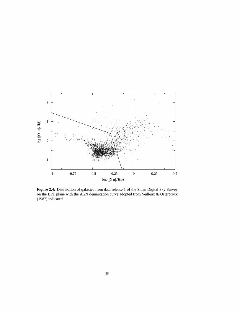
Using numerical models to quantify these differences, Baldwin et al. (1981)and Veilleux & Osterbrock (1987) developed emission line diagnostics to differen-tiate between AGN and star formation dominated emission line spectra. The morepractical diagnostics use ratios of close by and bright lines, typically [N II]/Hα vs[O III]/Hβ (the so called BPT diagnostic). This diagnostic was used in most ofthis work, with the curve dividing the AGN from star forming galaxies taken fromVeilleux & Osterbrock (1987) and approximated as a broken straight line definedby the point of the break, (xc,yc), and the slopes on the two sides of the break, b0

and b1. That is, the curve is defined as:

y =

{yc + b0(x− xc), x < xc

yc + b1(x− xc), x≥ xc.(2.14)

The values of these parameters are given in Table 2.1. Also indicated in this tableare the parameters used in the to classify objects on the [O I]/Hβ vs. [N II]/Hαplot. The distribution of galaxies from the Sloan Digital Sky Survey (see Section 5)on the [N II]/Hα vs [O III]/Hβ plane is shown in Figure 2.4 together with theadopted line separating AGN-dominated from star formation-dominated galaxies.

17

00

2020

4040

6060

8080

100100F

lux

Den

sity

(10−

17

Wm−

2)

Flu

xD

ensi

ty(

10−

17

Wm−

2)

50005000 55005500 60006000 65006500 70007000 75007500

Wavelength (A)Wavelength (A)

Figure 2.3: A part of the SDSS spectrum of the starburst galaxy SDSS J001630-111123.

Table 2.1: Parameters of curves dividing AGN from starbursts.

x y xc yc b0 b1

log([N II]/Hα) log([O III]/Hβ ) -0.28 0.38 -1.51 -13.6log([O I]/Hα) log([O III]/Hβ ) -1.08 0.52 -0.75 -1.59

18

−1−1

00

11

22

log

([O

iii]/Hβ

)lo

g([

Oii

i]/Hβ

)

−1−1 −0.75−0.75 −0.5−0.5 −0.25−0.25 00 0.250.25 0.50.5

log ([N ii]/Hα)log ([N ii]/Hα)

Figure 2.4: Distribution of galaxies from data release 1 of the Sloan Digital Sky Surveyon the BPT plane with the AGN demarcation curve adopted from Veilleux & Osterbrock(1987) indicated.

19

20

Chapter 3

Modelling Nuclear Starbursts

3.1 Introduction

It is quite clear even from optical photographs of galaxies, where ‘dust lanes’ areoften seen, that dust absorption will significantly influence observed properties ofgalaxies. Besides trying to correct the ultraviolet, optical and sometimes near-infrared observations for the effects of absorption and scattering, it is clearly be-neficial to make use as far as possible of dust emission to examine the propertiesof the excitation source and conditions in the interstellar medium. In some highlyobscured galaxies, like ULIRGs and the SCUBA galaxies, this may in fact be theonly way of understanding the properties of the population rather than just a fewsources.

The first on the wish-list of information one may hope to extract from dustemission is the total power absorbed by the dust, and thus in the heavily obscuredsystems at least, the power produced by whatever is heating the dust. The otherimportant question is the nature of the heating source: our ability to separatelydetermine the star formation history and black-hole growth history of the universemay depend on our ability to interpret mid-infrared spectra of heavily obscuredgalaxies to determine the balance between these two possible power sources.

It has already been noted that in the far-infrared, at wavelengths longer thanabout 50 µm, emission from dust takes the form a featureless continuum approx-imately corresponding to a modified black body, that is Sν ∝ λ−β Bν(T ). (Ob-served spectra of galaxies at these wavelength show, of course, in addition strongmolecular and atomic fine-structure lines which trace the gas phase rather than thedust.) When working with a small number of photometric measurements in fixedwavelength bands, especially if they are all in the Rayleigh-Jeans tail of emission,there will inevitably be significant uncertainty in the dust temperature, T , whichcorresponds to large uncertainties in the estimated total power output of the dust.

In contrast, the region of the spectrum dominated by transiently heated dust,3.3 µm/ λ / 40 µm, is populated by a number of broad emission features. Addi-tionally, emission from transiently heated dust, when compared to dust in equilib-

21

0.050.05

0.10.1

0.20.2

0.50.5

11

22

55

1010

2020

5050

Fν

(Jy)

Fν

(Jy)

6 · 10−66 · 10−6 8 · 10−68 · 10−6 1 · 10−51 · 10−5 1.2 · 10−51.2 · 10−5 1.4 · 10−51.4 · 10−5

λ (m)λ (m)

Figure 3.1: Mid-infrared spectra (all measured in an 9′′×9′′ aperture) of the nuclear regionof M 82 (solid line), an off-nuclear region of M 82 (dotted line, 30′′ from the nucleus)and the nuclear region of NGC 1068 (dashed line). All are from ISO observations withISOCAM in the CVF mode (the glitch around 9.2 µm is due to scanning pattern of thefilter). Data presented here are ‘HPDP’ version obtained from the ISO data archive.

rium, depends in a very different way on the radiation field and dust geometry (thisis illustrated later in Figure 3.6), and therefore, highly complementary informationcan be extracted from mid-infrared and far-infrared observations. For example, thelarge equivalent-widths of the PAH emission features (often > 1 µm) and silicateabsorption makes it possible to measure efficiently redshifts using low-resolutionspectroscopy or photometry.

The wealth of information in the mid-infrared spectra, however, also means thata full interpretation is difficult. As an illustration, three mid-infrared spectra takenby ISO are shown in Figure 3.1. One of the spectra shows emission from the nuc-lear region of the nearby prototype starburst galaxy M 82 (Forster Schreiber et al.,2003; Walter et al., 2002), the second is of a region in the disk of the same galaxyand the third is of the nucleus of the prototype Seyfert 2 galaxy NGC 1068. Themost striking difference between these spectra is the complete lack of PAH featuresin the spectrum of NGC 1068 which instead is dominated by a rising continuumextending throughout the measured spectral range. Some differences between thenuclear and off-nuclear spectra of M 82 can also be seen: the 11.3 µm PAH featureis depressed relative to the other features in the nuclear spectrum, but significantlyless so in the off-nuclear spectrum.

22

Existing models

Significant progress has been made in interpreting dust emission with a variety ofempirical approaches. At far-infrared, sub-millimetre and millimetre wavelengths,the usual technique is fitting a number (one, two, or even three) modified black-body spectra of the form Bνλ β (e.g., Dunne et al., 2000; Blain et al., 2003). It isgenerally found that at least two components are required (Fitt et al., 1988); thewarmer component is usually taken to be associated with dust heated by a starburstwhile the cooler component is associated with ‘cirrus-like’ dust that is heated by thegeneral interstellar radiation field. It is shown later that even the simplest radiativetransfer through dust gives rise to a wide range of dust temperatures and, of course,the emissivity of dust in the far infrared and sub-millimetre is a strong function ofdust sizes. Therefore, although the above mentioned models provide reasonable fitsto the observed data, it is not clear if they can be literally interpreted as describingthe physical conditions of the dust.

In the mid-infrared, the widely used approach is to use observed spectra astemplates for fitting. The large wavelength coverage of the grating spectrometerSWS on ISO was particularly useful for providing these templates (Sturm et al.,2000) although necessarily restricted to the nearby bright objects. As noted inthe introduction, Laurent et al. (2000) used this approach to produce mid-infrareddiagnostics (suitable for both spectroscopy and photometric measurements) to dis-tinguish between dominant heating sources of the dust. Further, combinations oftemplate spectra have used to fit the observed spectra of individual objects, by forexample Spoon et al. (2004) who modelled Arp 220 in this way.

Finally a number of authors have begun developing physically-based modelsfor dust emission from galaxies. Silva et al. (1998) present a radiative transfer anddust model which they used to model infrared emission from galaxies. A similarmodel is presented by Siebenmorgen et al. (1999). Although both of these modelstreat transiently heated grains neither does so with great resolution or detail. Themodel by Siebenmorgen et al. (1999) for example only considers PAHs of a singlesize while Silva et al. (1998) do not resolve the emission from individual features.

Closest to the models presented in this chapter are ones presented by Misseltet al. (2001) and Gordon et al. (2001). The main difference between those mod-els and those presented here are that they treat radiative transfer in greater detail,including for example heating of dust by absorption of mid-infrared radiation anddetailed scattering calculations. The present models, however, treat emission fromPAHs (which dominates the mid-infrared wavelengths) in significantly more detailby, for example calculating the full internal energy probability distribution for anumber of molecule sizes and making use of physically motivated normal-modespectra to calculate heat capacities.

23

Modelling

In this chapter, models of emission from obscured star forming regions are de-veloped with particular emphasis on mid-infrared emission from dust. A simpleshell geometry is adopted for all of the models. Dust obscuration is fully consist-ently calculated using the same dust model used to calculate dust emission. Re-absorption of dust emission, however, is not taken into account when calculatingthe spectrum of emission. The effect of this is to significantly underestimate theemissivities in the far infrared and sub-millimetre regions of the spectrum; there-fore, the calculated spectra in these regions should be taken as lower limits. Thesemodels are then applied to two systems in Chapter 4, making use of new high-resolution mid-infrared imaging to constrain the sizes of dust shells used.

The dust heating sources are modelled to be point-like with properties derivedfrom stellar synthesis models described in Section 3.2. The main sources for thedust model, from which absorption cross sections and dust emissivities are derived,are the excellent series of papers by B.T. Draine and collaborators: Draine & Li(2001); Li & Draine (2001); Weingartner & Draine (2001a). The model itself isdescribed in Section 3.3 while some illustrative derived spectra are presented inSection 3.4.

3.2 Stellar radiation

The aim of this chapter is primarily to model obscured and relatively intenselystar forming galaxies which are to a large extent dominated by their young stellarpopulations. For this reason, stellar contents of these galaxies have been modelledusing the STARBURST99 spectral synthesis code by Leitherer et al. (1999). As thename suggests, this code is specifically designed to model intensely star formingsystems and is often used in the literature. The outputs provided by STARBURST99are: stellar spectral energy distribution, mechanical power due to stellar winds,supernova rates, and various derived properties such as integrated colours. All ofthese are produced at an arbitrary temporal resolution. The code on its own, how-ever, does not treat formation of emission lines or the effects of dust obscuration.

The two star formation scenarios treated in the STARBURST99 code are con-tinuous star formation with a fixed SFR and instantaneous formation in which allof the stars form at the same time. The results of these simulations can if necessarybe convolved to produce other star-formation rate histories. The most importantinput parameter to the code is the star-formation rate (for continuous star form-ation models) or the total mass of formed stars (for instantaneous star formationmodels). Some of the other parameters are:

• The slope of the initial mass function (Section 2.1) of the formed stars andthe lower and upper mass cutoffs. Only a single power-law type IMF issupported.

• Metallicity.

24

1 · 10351 · 1035

2 · 10352 · 1035

5 · 10355 · 1035

1 · 10361 · 1036

2 · 10362 · 1036

5 · 10365 · 1036

1 · 10371 · 1037

λLλ

(W)

λLλ

(W)

5 · 1025 · 102 1 · 1031 · 103 2 · 1032 · 103 5 · 1035 · 103 1 · 1041 · 104 2 · 1042 · 104 5 · 1045 · 104

λ (A)λ (A)

Figure 3.2: The spectral energy distribution of a starburst forming stars at a rate of1M� yr−1. Standard Salpeter (1955) IMF has been assumed with lower and upper masscutoffs of 1 M� and 100 M� respectively. The three traces correspond, from bottom to top,to epochs 107, 5×107 and 108 years after the onset of star formation.

Unless otherwise noted, all of the results presented here have been calculated usingthe Salpeter (1955) slope (that is, α =−2.35) and solar metallicity. It is quite likelythat the uncertainties in these parameters dominate any errors inherent in the code.

3.2.1 Starbursts

Figures 3.2 and 3.3 show how the spectral energy distribution of stars in a starburstevolves with time for continuous and instantaneous star formation models respect-ively. The parameters of the models are entirely ‘standard’: Salpeter (1955) IMFslope, 1 M� and 100 M� IMF cut-offs, and solar metallicity.

Many of the important features of stellar evolution can be seen quite clearly inthese plots. The very high ionising flux that is seen in the 2 Myr old instantaneousburst in Figure 3.3 is responsible for the Hα and other recombination-line emis-sion from young bursts. The ionising flux of the 16 Myr burst is essentially zero,showing that recombination lines are a good measure of very recent star formation.The rapid decline with time of total luminosity of the instantaneous burst can alsobe seen in Figure 3.3; the opposite of course holds for the continuous burst sincethe total mass of stars increases with time in this case. Both the continuous and in-stantaneous bursts show the emergence of the Balmer, or 4000 A, break indicativeof intermediate age stars.

25

10331033

10341034

10351035

10361036

10371037

λLλ

(W)

λLλ

(W)

5 · 1025 · 102 1 · 1031 · 103 2 · 1032 · 103 5 · 1035 · 103 1 · 1041 · 104 2 · 1042 · 104 5 · 1045 · 104

λ (A)λ (A)

Figure 3.3: Temporal evolution of the spectral energy distribution of an instantaneousstarburst of total mass 106 M�; the traces show the SED at times (top to bottom) 2× 106,16×106, and 98×106 years after the burst. The IMF is the same as in Figure 3.2.

3.2.2 Old stellar population

It is only in the most extreme starburst galaxies that the contribution of the oldstellar population can be completely neglected. In more modest starbursts, the oldstellar population will contribute most of the light in the optical and near-infraredwavebands and therefore proper calculation of both dust heating and near infraredluminosities must take them into account.

Several approaches can be taken in modelling the old stellar population: theSTARBURST99 models can be evolved to very old ages—this is shown in Fig-ure 3.4—or observed spectra of elliptical galaxies can be used. This figure illus-trates the reddening of the stellar SED and overall decrease in bolometric luminos-ity.

3.3 The dust model

The dust model that is developed in this section is based on calculating the proper-ties of grains, and their response to incident light, separately for each of species ofgrains and for a number of grain sizes. The observable properties are then arrivedat by integration across the size distributions (which are different for each of thespecies) and integration across a range of ambient radiation fields. The aim is todevelop a dust model that is physical enough to be able to predict how the spectrumof infrared radiation changes, not only with changes of the illuminating light, but

26

10311031

10321032

10331033

10341034

10351035

λLλ

(W)

λLλ

(W)

5 · 1025 · 102 1 · 1031 · 103 2 · 1032 · 103 5 · 1035 · 103 1 · 1041 · 104 2 · 1042 · 104 5 · 1045 · 104

λ (A)λ (A)

Figure 3.4: Synthetic STARBURST99 stellar spectra 5×107, 109, and 1010 years after theburst of star formation.

also with changes of the dust properties, such as destruction of the smallest grains.As the processes governing the formation, destruction, and charging of inter-

stellar dust are still poorly understood, current dust models are phenomenologic-ally based; and certainly, the models being proposed in the literature are not unique(e.g., Zubko et al., 2004). Furthermore, although observations of sight-lines to anumber of standard stars have shown that properties of dust vary within the Galaxy,it is beyond the reach of current instrumentation to attempt to make such a charac-terisation for all but the very nearest external galaxies. In conclusion, it must em-phasised that whichever single dust model is chosen, large uncertainties are likelypresent.

Three species of interstellar grains (Draine, 2003) are used in the model:

• Spherical silicate grains. The broad 9.7 µm absorption feature attributed tosilicates indicates that these grains are predominantly amorphous.

• Spherical graphitic grains.

• Polycyclic Aromatic Hydrocarbons (PAHs, reviewed by Allamandola et al.,1989), which are basically sturdy planar molecules composed of joined ben-zene rings.

The latter two species, PAHs and graphitic spheres, are assumed to form a singlefamily with properties smoothly varying with the radius a from PAH-like at a� aξto purely graphitic (and sphere-like) at a� aξ . This transition is described by the

27

parameter ξ , so that the properties of grains are a linear combination of PAH-likeproperties with a weight ξ and graphitic properties with a weight (1− ξ ). Theparameter ξ is defined by the equation:

ξ (a) = (1−qgra)

{1.0 a < aξ(aξ/a)3 a≥ aξ

(3.1)

where aξ defines the radius at which the transition occurs and qgra is a constantwhich allows for particles with a� aξ to retain a degree of bulk graphite-likeproperties. Li & Draine (2001) find that a non-zero qgra = 0.01 is needed to explainemission from the diffuse interstellar medium in our galaxy.

3.3.1 Absorption cross sections

The absorption cross section describes the coupling between dust particles andphotons: power absorbed by a dust particle of cross section Cabs(λ ;a) in an iso-tropic radiation field with energy density uλ is simply Cabs(λ ;a)cuλ . For particleswith a well defined temperature, the power emitted is also simply related to the ab-sorption cross section and the Planck function, Bλ , so that the full energy balanceequation of the grain is described by (neglecting stimulated emission):

dUλdt

= Uλ =−Cabs(λ )cuλ +Cabs(λ )4πBλ (T ). (3.2)

Here, Uλ is the total energy in the radiation field.

Mie cross sections

For the species modelled as spherical grains, the absorption cross sections werecalculated using Mie theory (e.g., Bohren & Huffman, 1998). The implementationused is based on a publicly available1 code originally itself based on the code byBohren & Huffman (1998) but modified by B.T. Draine and P.J. Flatau. This codewas further modified for this study by imposing the geometric limit in the regimeλ < a/3000 and compatibility upgrades.

The complex dielectric functions required for as the input to the Mie codewere chosen following Li & Draine (2001): the graphite dielectric function2 ofLaor & Draine (1993) and the ‘smoothed UV astronomical silicate’ function3 ofWeingartner & Draine (2001a). These were implemented by linearly interpolatingthe available tabular data. The strong non-anisotropy of graphite was treated usingstandard 1/3-2/3 approximation. In this approximation, the cross section of thegraphitic spheres is the weighted average of the Mie result using the dielectricfunction appropriate to the electric field being perpendicular and parallel to thegraphite plane, with 1/3 and 2/3 weights respectively.

1Available at http://atol.ucsd.edu/˜pflatau/scatlib/scatterlib.htm2Available at ftp://ftp.astro.princeton.edu/draine/dust/diel/eps Gra3Available at ftp://ftp.astro.princeton.edu/draine/dust/diel/eps suvSil

28

PAH cross sections

Absorption cross sections of PAHs are both difficult to measure in the laboratoryand difficult to calculate from first principles. Therefore, I used empirical absorp-tion cross sections determined by Li & Draine (2001). These cross sections area piece-wise combination of polynomials representing the continuum and a seriesof Drude profile representing the emission features. Two cross sections are given,representing neutral and ionised PAHs; the main difference between these two is inthe strength of the emission features in the 3–10 µm range. In particular the neutralPAHs have a stronger feature at 3.3 µm while the ionised PAHs have larger crosssections in the 6–9 µm complex.

The details of the implementation are given in Appendix A.1.1, so here onlythe important parameters are reviewed. These are the PAH feature enhancements,E6.2 µm, E7.7 µm and E8.6 µm which are needed to reconcile the properties of PAHs inthe laboratory with observations. I used the best-fitting values for the diffuse ISMof the Galaxy (Li & Draine, 2001): 3.0, 2.0 and 2.0 respectively.

3.3.2 Infrared emission from dust grains

Over a sufficiently long time period a dust grain must be in equilibrium with theambient EM field so that

〈∫

dλUλ 〉= 0, (3.3)

where Uλ energy in the EM field as defined in Equation 3.2. A naive calculationof dust emission—in fact only valid for quite large grains (a & 200 A) in a typicalinterstellar radiation field—would proceed by requiring Equation 3.3 holds at everyinstant in time and therefore solving for the dust temperature using the equation:

∫dλCabs(λ )cuλ =

∫dλCabs(λ )4πBλ (T ). (3.4)

It is now well known, however, that there is a significant population of smallgrains—the transiently heated grains—for which the cooling timescale is muchfaster than the rate at which they absorb photons and that they therefore exhibitvery large temperature fluctuations (Purcell, 1976; Sellgren, 1984; Draine, 2003).Therefore, Equation 3.4 does not in general hold for interstellar dust.

A more general approach, which can accurately model the transiently heatedgrains, is to consider the probability distribution of internal energy (or, more pre-cisely enthalpy) of the grain. In general, this is preferable to considering the prob-ability distribution grain temperature which is not easily defined the very smallgrains (which are essentially just single molecules). In the present model, how-ever, a one-to-one relationship between temperature and energy is established forall grains.

29

Energy bins and bin temperatures

The method for solving for the energy probability distribution of grain is based onthe approach of Guhathakurta & Draine (1989). This approach is shown by Draine& Li (2001), who refer to it as the ‘thermal-continuous’ model, to be in practicesufficiently accurate when compared to more exact methods.

The possible internal energy content of a grain is represented by a number Nof energy bins, where I have normally used N = 300. The low energy bins arecarefully chosen to represent the first few ground states of the grain (as was donein Draine & Li, 2001), with the later bins being first linear and then logarithmic inenergy. The last bin has a high enough energy that the grain has a vanishing prob-ability of reaching it. The quantity that we seek, the energy probability distributionof the grain, is represented by a vector Pi giving the probability that the grain is ina state that belongs to the i-th energy bin.

Energy bins were assigned representative temperatures, following Draine & Li(2001), in the following way. As at energies close to the ground state temperatureis poorly defined, so the first twenty bins were assigned a constant temperature,T1−20 = E1/(k log 2), where E1 is the energy of the first excited state. For grainswith less than 500 atoms and for the lower bins of larger grains, the temperatureswere calculated by finding the temperature that gives an energy expectation valuefor the grain equal to the bin energy. This was done using a Newton-Raphson typeminimiser with numerical derivatives and spectrum of normal modes described inAppendix A.1.2. Finally, in rest of the cases, the continuum Debye approximationwas used.

Transition matrix and solving for Pi

Information about the interaction of a grain with the EM field is contained in atransition matrix Ti j which gives the rate at which grain transitions from a statewith energy in the j-th bin to a state with energy in the i-th bin. Upward transitionscorrespond to absorption of photons and are given by:

Tul =c∆Eu

Eu−El

∫ W4

W1

dEGul(E)Cabs(E)uE . (3.5)

Here, as before, Cabs is the absorption cross section and uE is the energy densityof the radiation field. The factor Gul , which represents a correction for the finitewidth of energy bins, and the limits W1 and W4 are defined in Appendix A.1.3 andEu and El are the centre energies of upper and lower bins respectively. Finally ∆Eu

is the width of the upper energy bin.In the present approximation, the cooling of the grain is represented as cascade

from higher to lower energy bins one bin at a time. Therefore:

Tlu = 0 for u− l > 1. (3.6)

30

The non-zero downward transitions are given by:

Tu−1,u =1

Eu−Eu−1

8πh3c2

∫ Eu

0dE

E3Cabs(E)

exp(

EkTu

)−1

. (3.7)

Once the rates of up and down transitions are known it is quite straightforwardto evaluate the probability distribution of the grain being in a state in bin i (Guhath-akurta & Draine, 1989). This is primarily because a transition to any bin j suchthat j ≥ i guarantees, due to the single bin at a time downward cascade, that thegrain will reach bin i. Therefore, the matrix

B ji =N

∑u= j

Tui, (3.8)

where N is the total number of bins, gives an ‘effective’ transition rate from i-th to j-th bin which can then be used to evaluate the un-normalised probabilitydistribution, Pj, as follows:

Pj =1

Tj−1, j

j−1

∑i=0

PiB ji. (3.9)

Both of these operation can be done iteratively at a relatively small computationalcost of O(N2).

The emitted spectrum

Once the probability distribution Pi is known, the spectrum of radiation emitted bya grain can be calculated using:

Fν =2hν3

c2 Cabs(ν)

∑

u s.t. Eu>hν

Pu

exp(

hνkTu

)−1

(

1 +λ 3

8πuE

). (3.10)

The last factor in this equation is the generally negligible correction for stimulatedemission.

3.3.3 Size distribution of dust particles

The last piece of information required to calculate dust emission is the size distri-butions of dust particles. As the processes shaping interstellar dust grains are stillpoorly understood, our knowledge of these size distributions is based on primarilyon inference from observations of extinction and infrared emission. Clearly thisinference in itself depends on models like the one constructed in previous sections.The grain size distribution used in the models presented in this chapter are basedon those published by Weingartner & Draine (2001a). These in turn are based on

31

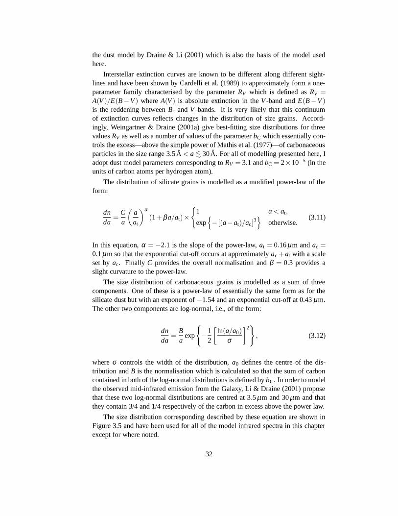
the dust model by Draine & Li (2001) which is also the basis of the model usedhere.

Interstellar extinction curves are known to be different along different sight-lines and have been shown by Cardelli et al. (1989) to approximately form a one-parameter family characterised by the parameter RV which is defined as RV =A(V )/E(B−V ) where A(V ) is absolute extinction in the V -band and E(B−V )is the reddening between B- and V -bands. It is very likely that this continuumof extinction curves reflects changes in the distribution of size grains. Accord-ingly, Weingartner & Draine (2001a) give best-fitting size distributions for threevalues RV as well as a number of values of the parameter bC which essentially con-trols the excess—above the simple power of Mathis et al. (1977)—of carbonaceousparticles in the size range 3.5 A < a. 30A. For all of modelling presented here, Iadopt dust model parameters corresponding to RV = 3.1 and bC = 2×10−5 (in theunits of carbon atoms per hydrogen atom).

The distribution of silicate grains is modelled as a modified power-law of theform:

dnda

=Ca

(aat

)α(1 + βa/at)×

{1 a< at,

exp{− [(a−at)/ac]

3}

otherwise.(3.11)

In this equation, α = −2.1 is the slope of the power-law, at = 0.16 µm and ac =0.1 µm so that the exponential cut-off occurs at approximately ac + at with a scaleset by ac. Finally C provides the overall normalisation and β = 0.3 provides aslight curvature to the power-law.

The size distribution of carbonaceous grains is modelled as a sum of threecomponents. One of these is a power-law of essentially the same form as for thesilicate dust but with an exponent of −1.54 and an exponential cut-off at 0.43 µm.The other two components are log-normal, i.e., of the form:

dnda

=Ba

exp

{−1

2

[ln(a/a0)

σ

]2}, (3.12)

where σ controls the width of the distribution, a0 defines the centre of the dis-tribution and B is the normalisation which is calculated so that the sum of carboncontained in both of the log-normal distributions is defined by bC. In order to modelthe observed mid-infrared emission from the Galaxy, Li & Draine (2001) proposethat these two log-normal distributions are centred at 3.5 µm and 30 µm and thatthey contain 3/4 and 1/4 respectively of the carbon in excess above the power law.

The size distribution corresponding described by these equation are shown inFigure 3.5 and have been used for all of the model infrared spectra in this chapterexcept for where noted.

32

0.10.1

0.20.2

0.50.5

11

22

55

1010

2020

5050

100100

1029a

4n−

1H

dnda

(cm−

3)

1029a

4n−

1H

dnda

(cm−

3)

10−410−4 10−310−3 10−210−2 10−110−1 100100

a(µm)a(µm)

0.10.1

0.20.2

0.50.5

11

22

55

1010

2020

5050

100100

1029a

4n−

1H

dnda

(cm−

3)

1029a

4n−

1H

dnda

(cm−

3)

10−410−4 10−310−3 10−210−2 10−110−1 100100

a(µm)a(µm)

Figure 3.5: The size distribution of carbonaceous (top) and silicate (bottom) interstellardust grains that corresponds to RV = 3.1 and bC = 2×10−5 and best fits the observationsof diffuse emission in the Galaxy and extinction (plot units follow Weingartner & Draine2001a).

33

10−710−7

10−610−6

10−510−5

10−410−4

10−310−3

10−210−2

Sν4πD

2(W

Hz−

1m

2H−

1)

Sν4πD

2(W

Hz−

1m

2H−

1)

10−610−6 10−510−5 10−410−4 10−310−3

λ (m)λ (m)

Figure 3.6: Dust emissivity for optically thin dust shells with radii 0.01, 0.05, 0.2, 0.5,1, 2, and 5 kpc. The heating source is a 108 yr old starburst which has been forming starsat 1 M� yr−1. PAH ionisation has been fixed at 80%. Emissivity has been expressed perhydrogen atom and integrated over the area of the shell.

3.4 Simulated spectra

3.4.1 Optically thin limit

The computationally simplest approximation is to assume that the column densityof dust surrounding the source is so small that it has a negligible impact on the ra-diation field. For a point source of the exciting radiation the only factor controllingthe radiation field, and therefore dust emission, at any point is its distance from theexciting source. For solar-metallicity star-forming galaxies this is probably nevera good approximation since dust cross section to far-ultraviolet radiation is veryhigh. Even so, this approximation is sufficiently good to provide insight into someimportant factors that control infrared emission from dust.

Infrared emissivity of dust in thin shells at a number of radii from heatingsource are shown in Figure 3.6. The heating source is a ‘canonical’ starburst whichhas been continuously forming stars at a rate of 1 M� per year for 108 yr. Sincethe dust is assumed to be optically thin to the exciting radiation, its total infraredluminosity is simply proportional to the total number of hydrogen atoms in theshell. The spectra are expressed in units Sν4πD2 where Sν is dust emissivity perhydrogen atom so that the total luminosity can be obtained by simply multiplyingplotted values by the hydrogen column density of the shell.

The spectra in Figure 3.6 illustrate many of the important concepts of infrared

34

10−1210−12

10−1010−10

10−810−8

10−610−6

10−410−4

10−210−2

Sν4πD

2(W

Hz−

1m

2)

Sν4πD

2(W

Hz−

1m

2)

10−610−6 10−510−5 10−410−4 10−310−3

λ (m)λ (m)

Figure 3.7: Dust emissivity for an optically thin dust shell of radius 1 kpc excited by a106 M� starburst situated at the centre of the shell. The three traces correspond to starburstages 2×106, 16×106, and 98×106 years (the excitation spectra are shown in Figure 3.3).

emission from interstellar dust. In the far-infrared (λ ' 30 µm) emission can beapproximated by a modified black-body law with the Rayleigh-Jeans tail approx-imately following fν ∝ ν−(2+β ) with β ≈ 1.7. The peak of the modified black bodyis approximately at 20 µm for the shell at radius 10pc and 150 µm for the shell at5kpc. This behaviour can be explained by a simple analysis as follows. Sinceonly geometric dilution controls the radiation field, the energy density has the formu ∝ D−2 where D is distance from the heating source. According to Wien’s lawλpeak ∝ T and for a modified black body T 4+β ∝ u. Therefore λpeak ∝ D−2/(4+β )

which is very close to the observed behaviour.Shortward of the far-infrared peak, emission from dust shows a marked excess

compared to what would be expected from a black body. Particularly prominent arethe PAH emission features at 3.3, 7.7 and 11.3 µm, but the continuum too is alsowell above what would be expected from a black body in equilibrium. Furthermore,the intensity and shape of the mid-infrared spectrum changes very little with theshell radius. For example, the strength of the 7.7 µm emission feature changes byabout 30% while the radiation field energy density varies by a factor of 2.5×105.

The reason for this behaviour shortward of the black body peak are of coursethe transiently heated grains; they usually cool completely to the ground statebetween absorptions of photons and hence are completely insensitive to the energydensity of the radiation field. Rather, the emission is more sensitive on the spec-trum of the heating radiation. This is illustrated in Figure 3.7 which shows how theemissivity of dust changes as a starburst ages. It can be seen that the intensity of

35

the PAH features declines by about three orders of magnitude as the starburst agesfrom 2× 106 to 98× 106 years. By comparison, dust emissivity in the sub-mmregion changes by only a factor of three over the same period. This is due to therapid decline in energetic UV photons, responsible for the transient heating, as thestarburst ages. The grains that contribute the most to sub-mm emission are largergrains which are in equilibrium and have a large cross section to optical radiation.

3.4.2 Destruction of small grains

One often discussed interpretation of the variety of huge variety in observed mid-infrared spectra is processing of the dust grains by radiation, usually resulting withthe destruction of (very-) small grains. Using the above model this can be quiteeasily explored.

Figures 3.8 and 3.9 show dust emissivity for an optically thin shell with a ra-dius of 1 kpc and all other conditions as in Figure 3.6. The five traces on thesefigures correspond to correspond to five values of the smallest dust grains presentin the model, thereby simulating destruction of the grains (i.e., the size distributionis not renormalised so the total amount of material contained in dust is reduced).The effect of small-grain destruction in this relatively dilute radiation field is, asexpected, to reduce the intensity of mid-infrared emission. Most sensitive to de-struction of small grains is the emission at the shortest wavelengths; for example,destruction of grains in the 3.5 A–5 A radius range depresses the 3.3 µm feature bya factor of about five while the 11.3 µm feature shows a change of less than 10 per-cent. Notably, there is little change between the relative strengths of the continuumand features.

3.4.3 Reprocessing of PAHs I

Here I consider how the crossover between graphitic and PAH properties—whichis defined by the parameter aξ but occurs relatively smoothly over a range of grainradii (see Equation 3.1)—affects the emission from dust grains. Since Li & Draine(2001) find that this crossover is relatively poorly constrained by their models,it is of interest to investigate what if any effect it has on the models producedhere. More importantly, the graphitic grains have no PAH-like emission featuresand hence, any processing of the interstellar medium in such a way which woulddecrease aξ may contribute to the large variation in PAH feature to mid-infraredcontinuum ratios that are observed.

Initial investigation showed that variation in aξ down to as little as 20 A pro-duced negligible changes in the emission spectra. Therefore, I compare two quiteextreme crossover radii, 10 A and 4 A to the standard 50 A radius. Mid-infraredspectra corresponding to these three models are shown in Figure 3.10 for moderatestarburst conditions and dust shell of radius 1 kpc, i.e., in a regime where transi-ent heating is completely dominant in the grains which contribute to mid-infraredemission. It can be seen that even for aξ = 10, little change is seen in the emission

36

10−710−7

10−610−6

10−510−5

10−410−4

10−310−3

10−210−2Sν4πD

2(W

Hz−

1m

2H−

1)

Sν4πD

2(W

Hz−

1m

2H−

1)

10−610−6 10−510−5 10−410−4 10−310−3

λ (m)λ (m)

Figure 3.8: Dust emissivity for conditions as in Figure 3.6 (rshell = 1kpc) but for fivevalues of radius of the smallest dust grains present in the model (from top to bottom):3.5 A, 5 A, 7 A, 10 A, and 15 A.A

10−710−7

10−610−6

10−510−5

10−410−4

10−310−3

Sν4πD

2(W

Hz−

1m

2H−

1)

Sν4πD

2(W

Hz−

1m

2H−

1)

1 · 10−51 · 10−5 2 · 10−52 · 10−5

λ (m)λ (m)

Figure 3.9: Detail of Figure 3.8 showing the main PAH emission features.

37

1 · 10−51 · 10−5

2 · 10−52 · 10−5

5 · 10−55 · 10−5

1 · 10−41 · 10−4

2 · 10−42 · 10−4

5 · 10−45 · 10−4

1 · 10−31 · 10−3

Sν4πD

2(W

Hz−

1m

2H−

1)

Sν4πD

2(W

Hz−

1m

2H−

1)

1 · 10−51 · 10−5 2 · 10−52 · 10−5

λ (m)λ (m)

Figure 3.10: The effect of aξ , the radius at which the crossover between graphitic andPAH properties occurs: aξ = 4A is shown by the solid line; aξ = 10A by the dotted line;aξ = 50A by the dashed line. Excitation is as in Figure 3.6 for a shell of radius 1 kpc.

shortward of 11.3µm. For aξ = 4 however, there is a sharp change in the observedspectrum with the continuum becoming much more prominent.

The same calculation was repeated for a much more intense radiation fieldwhere even quite small grains can reach equilibrium. The results, presented inFigure 3.11, are qualitatively similar to those for a moderate radiation field, exceptfor the perceived shape of the continuum for the aξ = 4 crossover radius, which forthese conditions is clearly rising throughout the wavelength range shown.

3.4.4 Reprocessing of PAHs II

The simplest scenario for destruction of small grains has already been treated inSection 3.4.2, where it was assumed that all grains smaller than a particular size arevapourised. As it will be shown later, such models of the dust grain population havesome, but not complete, success in matching observations. Therefore, I proposehere a different way of modelling of breakdown of small grains, based in part onsome physical consideration.

It has already been noted that larger grains are in approximate equilibrium withthe radiation field, and further more, they do not show strong emission featureslike the PAHs. Therefore, they contribute mostly to the featureless far-infraredcontinuum and little information about their properties can be gained from mid-infrared observations, to which they generally contribute very little anyway. Theirproperties and size distributions are generally constrained from extinction and oc-

38

1 · 10−51 · 10−5

2 · 10−52 · 10−5

5 · 10−55 · 10−5

1 · 10−41 · 10−4

2 · 10−42 · 10−4

5 · 10−45 · 10−4

1 · 10−31 · 10−3

2 · 10−32 · 10−3

5 · 10−35 · 10−3

1 · 10−21 · 10−2

Sν4πD

2(W

Hz−

1m

2H−

1)

Sν4πD

2(W

Hz−

1m

2H−

1)

1 · 10−51 · 10−5 2 · 10−52 · 10−5

λ (m)λ (m)

Figure 3.11: As Figure 3.10 but for a shell of radius 50 pc.

casionally sub-mm observations. Instead I concentrate here on the very smallgrains.

In the dust model that is presently used, the size distribution of small grains,i.e., those with radii less than about 100 A, is determined by the two log-normal dis-tributions (described in Section 3.3.3) centred at 3.5 A and 30 A. In addition, thereis a sharp cutoff at 3.5 A which is based on the assumption that this is essentiallythe smallest size of PAHs (according to the present model, this radius correspondsto only twenty carbon atoms) that exists. If the log-normal distributions are inter-preted in terms of continuous processing of grains in the ISM, their peaks may beinterpreted as correspond to grain sizes which have a relatively long lifetime in theISM. Remembering that the size distribution given in Section 3.3.3 was derived forthe diffuse Galactic ISM, it is possible that the distribution is different in more ex-treme conditions. Without a fuller understanding of the physics of dust grains it isdifficult to predict how environmental conditions affect the grains. I again adopt avery simple model, in which accelerated break up of grains that may occur in moreextreme environments is modelled by a shift in central radii of the two log-normaldistributions of grains that I use. Using a common fractional shift for both of thedistributions, this process can be described by a single parameter γ . Changes of thesize distribution with this parameter are illustrated in Figure 3.12.

The effect such processing of dust grains has on mid-infrared spectra are shownin Figures 3.13 and 3.14, which show emissivity from the usual 1 kpc-radius dustshell heated by a moderate 1M� yr−1 starburst. As can be seen from these figures,emissivity at wavelengths longer than about 15 µm is not substantially changed forany value of the fractional shift in the log-normal distributions. The strongest effect

39

0.10.1

0.20.2

0.50.5

11

22

55

1010

2020

5050

100100

1029a

4n−

1H

dnda

(cm−

3)

1029a

4n−

1H

dnda

(cm−

3)

10−410−4 10−310−3 10−210−2 10−110−1 100100

a(µm)a(µm)

Figure 3.12: Size distribution of carbonaceous grains with processing modelled by shift-ing the centres of the log-normal distributions (see text for details); the lines show size-distributions corresponding to the following fractional shifts (i.e., γ) of log-normal distri-butions: 1.0 (full line, standard value), 0.8 (dashed line), 0.6 (dotted line), 0.4 (dash-dottedline).

10−710−7

10−610−6

10−510−5

10−410−4

10−310−3

10−210−2

Sν4πD

2(W

Hz−

1m

2H−

1)

Sν4πD

2(W

Hz−

1m

2H−

1)

10−610−6 10−510−5 10−410−4 10−310−3

λ (m)λ (m)

Figure 3.13: Dust spectrum corresponding to radiation field conditions as in Figure 3.6but with the carbonaceous grain size distributions as shown in Figure 3.12 (the meaning ofthe line-styles is as in that figure).

40

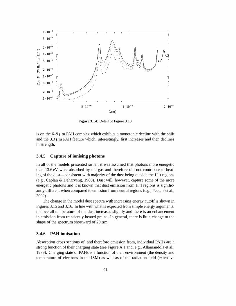
1 · 10−61 · 10−6

2 · 10−62 · 10−6

5 · 10−65 · 10−6

1 · 10−51 · 10−5

2 · 10−52 · 10−5

5 · 10−55 · 10−5

1 · 10−41 · 10−4

2 · 10−42 · 10−4

5 · 10−45 · 10−4

1 · 10−31 · 10−3

Sν4πD

2(W

Hz−

1m

2H−

1)

Sν4πD

2(W

Hz−

1m

2H−

1)

5 · 10−65 · 10−6 1 · 10−51 · 10−5 2 · 10−52 · 10−5

λ (m)λ (m)

Figure 3.14: Detail of Figure 3.13.

is on the 6–9 µm PAH complex which exhibits a monotonic decline with the shiftand the 3.3 µm PAH feature which, interestingly, first increases and then declinesin strength.

3.4.5 Capture of ionising photons

In all of the models presented so far, it was assumed that photons more energeticthan 13.6 eV were absorbed by the gas and therefore did not contribute to heat-ing of the dust—consistent with majority of the dust being outside the H II regions(e.g., Caplan & Deharveng, 1986). Dust will, however, capture some of the moreenergetic photons and it is known that dust emission from H II regions is signific-antly different when compared to emission from neutral regions (e.g., Peeters et al.,2002).

The change in the model dust spectra with increasing energy cutoff is shown inFigures 3.15 and 3.16. In line with what is expected from simple energy arguments,the overall temperature of the dust increases slightly and there is an enhancementin emission from transiently heated grains. In general, there is little change to theshape of the spectrum shortward of 20 µm.

3.4.6 PAH ionisation

Absorption cross sections of, and therefore emission from, individual PAHs are astrong function of their charging state (see Figure A.1 and, e.g., Allamandola et al.,1989). Charging state of PAHs is a function of their environment (the density andtemperature of electrons in the ISM) as well as of the radiation field (extensive

41

10−710−7

10−610−6

10−510−5

10−410−4

10−310−3

Sν4πD

2(W

Hz−

1m

2H−

1)

Sν4πD

2(W

Hz−

1m

2H−

1)

10−610−6 10−510−5 10−410−4 10−310−3

λ (m)λ (m)

Figure 3.15: Variation in dust spectrum with the cut-off energy of the radiation: 13.6 eV(the usual cut-off, solid line); 20 eV (dashed line); 30 eV (dot-dash line). The excitingradiation field is a 2 Myr old instantaneous starburst of total mass 106 M� and the shell hasa radius of 0.5 kpc.

10−710−7

10−610−6

10−510−5

10−410−4

10−310−3

Sν4πD

2(W

Hz−

1m

2H−

1)

Sν4πD

2(W

Hz−

1m

2H−

1)

1 · 10−51 · 10−5 2 · 10−52 · 10−5

λ (m)λ (m)

Figure 3.16: Detail of Figure 3.15.

42

1 · 10−61 · 10−6

2 · 10−62 · 10−6

5 · 10−65 · 10−6

1 · 10−51 · 10−5

2 · 10−52 · 10−5

5 · 10−55 · 10−5

1 · 10−41 · 10−4

2 · 10−42 · 10−4

5 · 10−45 · 10−4

1 · 10−31 · 10−3

Sν4πD

2(W

Hz−

1m

2H−

1)

Sν4πD

2(W

Hz−

1m

2H−

1)

5 · 10−65 · 10−6 1 · 10−51 · 10−5 2 · 10−52 · 10−5

λ (m)λ (m)

Figure 3.17: Variation in mid-infrared dust emissivity with ionisation fraction of the PAHs:neutral (full line), 50% ionisation fraction (dashed line), fully ionised (dotted line). Heatingsource as described in Figure 3.6.

discussion of grain charging is presented by Weingartner & Draine, 2001b); forthis reason it has not been explicitly calculated but treated as a free parameter.For the models presented so far I have adopted an ionisation fraction (assumed thesame for all grain sizes) of 0.8 corresponding to what Draine & Li (2001) find isappropriate for photo-dissociation regions. In Figure 3.17 I show the variation inthe emitted spectrum when this ionisation fraction is varied. As can be seen in thisfigure, the most sensitive tracer of the ionisation state is the 3.3 µm PAH emissionfeature.

3.4.7 Optically thick to exciting radiation

Dust shells which are optically thick to the exciting radiations were treated in thesimple approximation that disregards scattering of light by the dust and only con-siders absorption. Therefore, if Cint

abs(λ ) is the total absorption cross section of thedust, the exciting spectrum at column density of x into the shell is:

Sν(x) = Sν(0)exp[−xCint

abs(λ )]. (3.13)

The effects this attenuation of exciting radiation has on the emitted dust spectrum isillustrated in Figure 3.18 which shows how the dust spectrum for same conditionsas in Figure 3.6 changes as the exciting radiation travels through dust. It can beseen that mid- and far- infrared emissivity begin to rapidly decline in the column

43

10−1510−15

10−1210−12

10−910−9

10−610−6

10−310−3

100100

Sν4πD

2(W

Hz−

1m

2)

Sν4πD

2(W

Hz−

1m

2)

10−610−6 10−510−5 10−410−4 10−310−3

λ (m)λ (m)

Figure 3.18: Dust emissivity for a dust shell of radius 1 kpc excited by a starburst as de-scribed in 3.2 attenuated by dust column densities 0.01, 0.1 , 0.5 , 1, 5, and 10×1026 Hm−2.

density range 1025–1026 Hm−2. It can also be seen that the far-infrared peak moveslongwards as expected.

By integrating with column density it is possible to calculate the total emissionfrom a dust shell; this is shown in Figure 3.19 for four values of column density.This figure illustrates clearly that the majority of mid-infrared emission originatesin column densities 1024–1025 Hm−2 and that even at 100 µm essentially all ofthe emission originates in the range 1025–1026 Hm−2. It is only in the sub-mm re-gion that dust which is obscured by column densities greater than about 1026 Hm−2

significantly contributes to emission. This sub-mm emission from highly obscureddust also notably changes the slope of the Rayleigh-Jeans tail of the spectrum cor-responding to 1027 Hm−2.

44

10171017

10181018

10191019

10201020

10211021

10221022

10231023

I ν(W

Hz−

1)

I ν(W

Hz−

1)

10−610−6 10−510−5 10−410−4 10−310−3

λ (m)λ (m)

Figure 3.19: The emitted dust spectrum for a dust shell of radius 1 kpc excited by a star-burst as described in 3.2 and of thickness (bottom to top) 1024, 1025, 1026, and 1027 Hm−2.

45

46

Chapter 4

Mid-infrared observations andmodels

4.1 Ground-based mid-infrared observations

The Earth’s atmosphere is opaque to radiation with wavelengths from almost all ofthe infrared region of the electromagnetic spectrum. The major ‘windows’ of at-mospheric transparency—themselves only accessible from very high and dry siteslike Mauna Kea and the Atacama desert—are centred at 10 µm (N-band), 18 µm(Q-band), 450 and 850 µm. The transmittance of the N-band window, shown inFigure 4.1, is high enough to allow sensitive and high-resolution observations fromthe ground.

Sample selection

Galaxies for MICHELLE narrow-band imaging were selected from the 12 µm-selected sample of Rush et al. (1993). The original sample consisted of twentyobjects but poor weather conditions meant that incomplete data, or no data at all,was obtained for all but one of the galaxies. New snapshot VLA radio continuumobservations were obtained where necessary for all of the galaxies so that consist-ent matched resolution four-frequency radio maps could be produced.

4.1.1 Data reduction

The observing strategy for ground-based mid-infrared imaging and spectroscopyneeds to cope with a very high, and highly variable, background signal. The originof this background is both the telescope itself and the atmosphere, with the lat-ter being responsible for most of the high frequency variation. The standard wayof removing this background signal is the ‘chop and nod’ technique, which wasemployed for all of our N-band observations.

This technique involves oscillation of the secondary mirror between two po-sitions such that the fields of view are offset by a small angle (15–20′′ , referred

47

00

0.20.2

0.40.4

0.60.6

0.80.8

11

Tra

nsp

are

ncy

Tra

nsp

are

ncy

5 · 1035 · 103 1 · 1041 · 104 1.5 · 1041.5 · 104 2 · 1042 · 104 2.5 · 1042.5 · 104 3 · 1043 · 104

Wavelength (nm)Wavelength (nm)

Figure 4.1: Atmospheric transmittance in the mid-infrared window. Data are courtesy ofthe Gemini Observatory, and have been produced from a radiative transfer model for theatmosphere with 1 mm water vapour.

to as the ‘chop-throw’) accompanied by synchronous readout of the detector arrayat each of the positions. The high frequency of the chopping motion (4.6 Hz atUKIRT, 5.3 Hz at Gemini), and very small variation of atmospheric emission onthe angular scales involved, means that differencing the frames taken at each po-sition effectively removes the atmospheric background and most of the telescopebackground. Needles to say, the differencing of frames also removes any emissionof astronomical origin that is extended on scales comparable to the chop-throw.

The different light paths through the telescope at the two chop positions will,however, leave a chop-synchronous signal which needs to be removed by a secondstage of differencing, using observations with the whole telescope pointed at asmall offset (usually the same as the chop-throw) from the object. The resultingdata will contain either four images of the object (two positive and two negative) ifthe offset of the telescope (‘nod’) is arranged to be perpendicular to the chop direc-tion (this was the case for UKIRT observations); or, three images (two negative andone positive) if the chop and nod directions are co-linear and of same magnitude(this is usually referred to as ‘beam-switching’, it was used for the Gemini obser-vations). Bright star observations illustrating both of these strategies are shown inFigure 4.2.

As the incoming radiation is split between the multiple images of the object,combining these can significantly improve the signal to noise ratio. If the fourimages are aligned along the rows and columns of the detector, as was the casefor the UKIRT observations, combining the images can also be effective at sup-

48

Figure 4.2: Double-differenced observations of standard stars at 11.6 µm showing mul-tiple positive and negative images: (a) αAri. with MICHELLE/UKIRT and (b) βPeg. withMICHELLE/Gemini (‘beam-switched’).

pressing column and row based noise. The combination is easily done using thePyRAF IMSHIFT and IMCOMBINE tasks. In order to minimise distortions due tomis-registration of the images, the offsets between images were calculated for thehigh signal to noise observations of standard stars, rather than relying on the nom-inal values of chop/nod throws and directions.

The guiding system of the Gemini telescope was only able to operate at oneof the chop positions when these data were taken. This resulted in significantdegradation in the quality of the negative images, which is visible in Figure 4.2b.Because of this, the above procedure of combination of the positive and negativeimages was omitted and only the positive-beam image was used.

Flux calibration

Observations in each filter were proceeded by observations of mid-infrared brightnearby standard stars. These observations were used both for flux density calibra-tion and measurement of the point spread function.

The standards used are shown in Table 4.1 together with their assumed N-bandmagnitudes. These were than converted in flux densities using the zero-point valueslisted in Table 4.2.

Flat-fielding

When using array detectors it is common practice, in order to maximise the accur-acy of the observations, to calculate and correct for the pixel-to-pixel variation ofthe detector gain (the ‘flat-field’ in optical terminology). For ground-based mid-IR observations, the night sky provides a suitable uniform source of illuminationneeded for this measurement. Because the sky is sufficiently bright, when the

49

Table 4.1: MICHELLE calibration sources

BS name Other Name N-band magnitudea

BS 5054 ζUMa 2.24BS 5340b αBoo -3.17BS 5793b αCrB 2.19BS 6705b γDra -1.50BS 8775b βPeg -2.54BS 0617 αAri -0.84a From UKIRT 10 µm bright standards listb Mauna Kea Primary Standard

Table 4.2: MICHELLE fil-ter zero-points, from UKIRTweb pages, following Tokun-aga (1984).

filter centre zero-pointµm Jy

7.7 65.38.7 53.09.8 42.3

10.1 39.810.3 38.511.6 30.512.5 26.4

50

Figure 4.3: Sky-flats constructed from median-filtered non-differenced observations at (a)7.9 µm and (b) 11.6 µm.

frames from the two chop beams are averaged rather than differenced, the domin-ant contribution to the measured signal will be the pixel response to this uniformsignal and this therefore allows estimation of the gain of each pixel.

Flat-fields, estimated using this technique, for 7.9 µm and 11.6 µm filters areshown in Figure 4.3. It should be emphasised that these are likely to be signific-antly affected by the dark-current and emissivity from the instrument; for example,the blotches apparent at the longer wavelengths (4.3b) are likely to be due to imper-fections in the optical train. This implies that the flat-field variations, which werefound to be of the order of 1 per cent root-mean-square (rms) at 7.9 µm and 2 percent rms at 11.6 µm, are to be understood as upper limits. Given the signal to noiseratios of our observations these variations are not a significant source of error andthe above flat-fields were not applied to the data.

A more accurate flat-field can be constructed by making observations at a num-ber of elevations and extracting the signal proportional to the airmass of observa-tions, i.e., cosecθ where θ is the elevation. While such observations are a partof the baseline calibration plan for Gemini, they had not been implemented forsemester 03B.

4.2 Results

The reduced mid-infrared images of all of the systems observed except NGC 520(which is treated in detail later) are presented below together with short notes.

51

Figure 4.4: MICHELLE observations of NGC 34; (a) 11.6 µm filter (Speak =61mJyarcsec−2 ); (b) 12.5 µm filter (Speak = 90mJyarcsec−2 ). Contours are at Speak×0.75n.

NGC 34

This is a disturbed system classified as LIRG and is at a recessional velocity of5931 km s−1. The mid-infrared images, shown in Figure 4.4, display some exten-ded structure which has also been reported in broad-band mid-infrared imaging byMiles et al. (1996).

NGC 7469

NGC 7469 is a well studied Seyfert galaxy with a prominent circum-nuclear star-burst. The images obtained with MICHELLE are shown in Figure 4.5; imaging ofthis system by Miles et al. (1996) shows similar structure to what is seen in ournarrow-band data while higher resolution imaging of this system has been presen-ted by Soifer et al. (2003) who show that nuclear emission originates from a regionabout 20 pc in size. Our 9.7 µm image is considerably more compact than im-ages in other filters, all of which contain strong PAH emission features. This isconsistent with what would be expected from the circum-nuclear starburst.

Arp 220

Arp 220 is an extremely well known disturbed system. It is discussed in detail inSection 4.4. The images presented in Figure 4.6 are in agreement with imaging bySoifer et al. (1999).

52

Figure 4.5: MICHELLE observations of NGC 7469; (a) 7.9 µm filter (Speak =250mJyarcsec−2 ); (b) 9.7 µm filter (Speak = 210mJyarcsec−2 ); (c) 11.6 µm filter(Speak = 270mJyarcsec−2 ); (d) 12.5 µm filter (Speak = 230mJyarcsec−2 ). Contours areat Speak×0.75n.

53

Figure 4.6: MICHELLE observations of Arp 220; (a) 7.9 µm filter (Speak =150mJyarcsec−2 ); (b) 9.7 µm filter (Speak = 46mJyarcsec−2 ); (c) 11.6 µm filter (Speak =41mJyarcsec−2 ). Contours are at Speak×0.75n.

54

Figure 4.7: MICHELLE observations of Makarian 231; (a) 9.7 µm filter (Speak =350mJyarcsec−2 ); (b) 11.6 µm filter (Speak = 445mJyarcsec−2 ). Contours are atSpeak×0.75n.

Makarian 231

The mid-infrared images of Makarian 231, a well known AGN-powered galaxy,are shown in Figure 4.7. They are unresolved, in agreement with imaging by, forexample, Miles et al. (1996).

NGC 5506

NGC 5506 is Seyfert 1 galaxy with a recessional velocity of 1853 km s−1 (e.g.,Nagar et al., 2002). Our mid-infrared imaging, shown in Figure 4.8, does notresolve the source as may be expected for a purely AGN-powered galaxy.

55

Figure 4.8: MICHELLE observations of NGC 5506; (a) 9.7 µm filter (Speak =230mJyarcsec−2 ); (b) 11.6 µm filter (Speak = 440mJyarcsec−2 ). Contours are atSpeak×0.75n.

56

4.3 Case study I: NGC 520

Galaxies for MICHELLE followup were selected from the 12 µm sample of Rushet al. (1993), which being a flux-limited sample contains galaxies with a wide rangeof intrinsic luminosities. The only galaxy for which, by the vagaries of the weather,we obtained a complete set of mid-infrared imaging with UKIRT was NGC 520,one of the lower luminosity members of our sample. It is catalogued as number 157in Arp (1966); as required for the membership of this catalogue, it has a distinctlypeculiar optical morphology with clear tidal tails and hints of a double nucleus.

Near infrared imaging of NGC 520 by Bushouse & Werner (1990, cataloguedas UGC 966) strikingly revealed two nuclei, particularly in the longest wavelength(K-band) image. A newer K-band image by Kotilainen et al. (2001) is shown inFigure 4.10 where the two nuclei are clearly visible. Also shown in Figure 4.10 isan R-band image by Xu et al. (2000) which shows that the brighter of the nucleiin the near-infrared, usually referred to as the ‘primary nucleus’ (PN), is almostcompletely obscured at optical wavelengths by a thick dust lane.

The disturbed morphology of this system has already suggested that NGC 520could be an intermediate- or late-stage merger—Toomre & Toomre (1972) includedit into their sequence of interacting galaxies—and the two near-infrared are nucleiare widely interpreted as nuclei of the progenitor galaxies (e.g., Stanford, 1990;Stanford & Balcells, 1991; Hibbard & van Gorkom, 1996). Numerical modellingof the H I distribution by Stanford & Balcells (1991) supports this interpretationand indicates that the merger commenced about 3×108 years ago.

4.3.1 Existing data

Partially because of its peculiar morphology and partially because of its mid-infraredbrightness, NGC 520 has been extensively studied in the past. Some of these dataprovide valuable constraints to the models presented later and are therefore re-viewed here. The recessional velocity of NGC 520 is 2282km s−1 (source: NED);for this analysis I adopt H0 = 70km s−1Mpc−1 and hence the distance to NGC 520of 33 Mpc; at this distance, one arcsecond on the sky corresponds to a physicalscale of approximately 160 pc.

IRAS observations

Fluxes and flux error estimates were obtained from the SCANPI service and areshown in Table 4.3. At the adopted distance, and using the prescription given bySanders & Mirabel (1996), these fluxes correspond to a total infrared luminosity inthe 8–1000 µm range of LIR = 1010.95 L�.

Neutral gas

NGC 520 was included in the study of neutral gas in interacting galaxies by Hib-bard & van Gorkom (1996) who derive total H I mass of 9.2×109 M� and total H2

57

Table 4.3: IRAS-SCANPI fluxes for NGC 520

Wavelength (µm) 12 25 60 100

Flux (Jy) 0.77 2.93 30.37 46.15Errora (Jy) 0.04 0.04 0.3 0.4a One percent systematic error has been added in

quadrature

mass of 18.0× 109 M�. In a followup study, Yun & Hibbard (2001) showed thatthe majority of the molecular hydrogen is concentrated in a torus of radius 500 pcaround the primary nucleus and that the peak surface density of molecular hydro-gen there is 3× 1023 cm−2. The same authors find no evidence for CO emissionin the region of the second (north-western) nucleus and place an upper limit of5×106 M� on the total mass of molecular gas there.

ISO observations

NGC 520 has been observed by ISO in a number of modes: the PHT-S mode ofISOPHOT producing a 2.5 to 12 µm spectrum (discussed in Lu et al., 2003); thewide field, broadband imaging mode of ISOCAM (discussed in Xu et al., 2000);and in the circular variable filter (CVF) mode of the ISOCAM producing a detailed6–15 µm data-cube. The broad-band wide-field mid-infrared imaging by Xu et al.(2000), which is shown as contours in Figure 4.10, has demonstrated that about90 percent of the mid-infrared luminosity of NGC 520 originates in the gas-richprimary nucleus.

The ISOCAM-CVF data, with their wide spectral coverage which includes allof the filters we used, are the most relevant to this work. Presented here are the‘Highly Processed Data Product (HPDP)’ version of the data (F. Boulanger, et al;in prep.) available in the ISO archive under observation number 77801902. Thesedata have been compared with the broad-band imaging in the LW7 filter by Xuet al. (2000) and found to disagree on the calibration by a factor of 1.58. The 6–15 µm spectrum, derived from these data, of the region surrounding the primarynucleus is shown in Figure 4.9. For comparison, also indicated in this figure asthe dashed line is a spectrum derived for the full field of view excluding the faultypixels.

As a calibration check, the ISO spectrum has been averaged over the MICH-ELLE filter pass-bands and compared to MICHELLE aperture photometry; theresults are shown in Table 4.4. A significant discrepancy is found between our dataand the ISOCAM-CVF data as obtained from the archive; however, once the CVFdata are corrected to the broad-band calibration of Xu et al. (2000), it can be seenthat the agreement is excellent.

58

0

0.5

1

1.5

2

2.5

3

Flu

xD

ensi

ty(J

y)

6 8 10 12 14

Wavelength (µm)

7.9 µm 9.7 µm 11.6 µm

12.5 µm

Figure 4.9: ISOCAM-CVF spectrum of NGC 520; solid line: spectrum of the 15′′× 15′′

region centred on the peak of emission; dashed line: spectrum of the full field of view.

Table 4.4: Flux densities, integrated over the central15′′×15′′ region, as observed by MICHELLE and ISO.

Wavelength (µm) 7.9 9.7 11.6 12.5

MICHELLE (Jy) 1.33 0.16a 0.70 1.25ISOb (Jy) 0.87 0.10 0.47 0.70ISOc (Jy) 1.28 0.16 0.75 1.11a Not a clear detection in imaging.b As obtained from the archive.c Corrected to calibration of Xu et al. (2000).

59

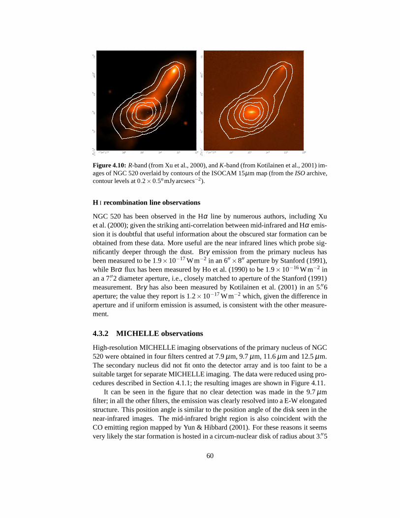
Figure 4.10: R-band (from Xu et al., 2000), and K-band (from Kotilainen et al., 2001) im-ages of NGC 520 overlaid by contours of the ISOCAM 15µm map (from the ISO archive,contour levels at 0.2×0.5n mJyarcsecs−2).

H I recombination line observations

NGC 520 has been observed in the Hα line by numerous authors, including Xuet al. (2000); given the striking anti-correlation between mid-infrared and Hα emis-sion it is doubtful that useful information about the obscured star formation can beobtained from these data. More useful are the near infrared lines which probe sig-nificantly deeper through the dust. Brγ emission from the primary nucleus hasbeen measured to be 1.9×10−17 Wm−2 in an 6′′×8′′ aperture by Stanford (1991),while Brα flux has been measured by Ho et al. (1990) to be 1.9×10−16 Wm−2 inan a 7.′′2 diameter aperture, i.e., closely matched to aperture of the Stanford (1991)measurement. Brγ has also been measured by Kotilainen et al. (2001) in an 5.′′6aperture; the value they report is 1.2×10−17 Wm−2 which, given the difference inaperture and if uniform emission is assumed, is consistent with the other measure-ment.

4.3.2 MICHELLE observations

High-resolution MICHELLE imaging observations of the primary nucleus of NGC520 were obtained in four filters centred at 7.9 µm, 9.7 µm, 11.6 µm and 12.5 µm.The secondary nucleus did not fit onto the detector array and is too faint to be asuitable target for separate MICHELLE imaging. The data were reduced using pro-cedures described in Section 4.1.1; the resulting images are shown in Figure 4.11.

It can be seen in the figure that no clear detection was made in the 9.7 µmfilter; in all the other filters, the emission was clearly resolved into a E-W elongatedstructure. This position angle is similar to the position angle of the disk seen in thenear-infrared images. The mid-infrared bright region is also coincident with theCO emitting region mapped by Yun & Hibbard (2001). For these reasons it seemsvery likely the star formation is hosted in a circum-nuclear disk of radius about 3.′′5

60

Table 4.5: Radio fluxes measured in box01h 24m 34.63s to 01h 24m 35.10s , +03◦ 47′ 27′′.9to +03◦ 47′ 32′′.0 from new and re-reduced VLA data.

Frequency (GHz) 1.42 4.86 8.46 14.9

Flux (mJy) 136.6 72.1 44.9 28.2

and vertical scale height of 1′′.The non-detection at 9.7 µm is consistent with the ISO spectrum shown in Fig-

ure 4.9. Aperture photometry of the image in this band does, however, produce apositive flux which is comparable to that measured by ISO. Comparison betweenthe ISO spectrum and aperture photometry of these data is detailed in Table 4.4 andaccuracy of calibration has been is discussed in Section 4.3.1.

VLA observations

Matched resolution radio maps of the primary nucleus were obtained1 using theVery Large Array at four frequencies: 1.4, 4.9, 8.5 and 15 GHz. They are presentedin Figure 4.12, overlaid on a gray-scale representation of 12.5 µm image.

4.3.3 Modelling

Number of ionising photons

With the wealth of data available, a number of avenues for estimating the numberof ionising photons are available; however, only the free-free luminosity providesa completely extinction free estimate so that is considered first.

Estimating the free-free luminosity is, of course significantly complicated bythe dominant presence of the synchrotron component, especially at low frequen-cies. With four flux measurements, it is however, possible to begin to disentanglethe contributions. Radio flux densities integrated across the disk are shown inTable 4.5 and Figure 4.13; these were used to estimate the synchrotron and free-free contributions to the radio emission (making use of the ANMAP package writ-ten by Dr P. Alexander). We find the synchrotron emission accounts for 127 of the136 mJy of emission at 1.42 GHz while the free-free component accounts for 7.8out of the 28.2 mJy of emission at 15 GHz. The position of the synchrotron spectralbreak, if it exists, is constrained to be νT > 25GHz.

Such a decomposition is consistent with the 0.′′2 resolution, 15 GHz, map ofthe primary nucleus by Carral et al. (1990) which shows that at least 5 mJy of fluxdensity at this frequency is associated with compact sources embedded in the disk

1These data are from new and archival observations. They were kindly reduced using standardinterferometric techniques by Dr M. Clemens of Padova University.

61

Figure 4.11: MICHELLE mid-infrared data, each observations is plotted in gray-scale andoverlaid with own contours; (a) 7.9µm filter (Speak = 109mJyarcsec−2 ); (b) 9.7µm filter(no detection, Speak = 28mJyarcsec−2 ); (c) 11.6µm filter (Speak = 44mJyarcsec−2 ); (d)12.5µm filter (Speak = 80mJyarcsec−2 ). Contours are at Speak×0.75n.

62

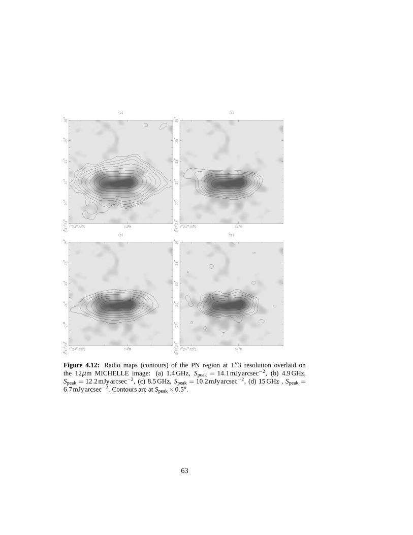
Figure 4.12: Radio maps (contours) of the PN region at 1.′′3 resolution overlaid onthe 12µm MICHELLE image: (a) 1.4 GHz, Speak = 14.1mJyarcsec−2, (b) 4.9 GHz,Speak = 12.2mJyarcsec−2, (c) 8.5 GHz, Speak = 10.2mJyarcsec−2, (d) 15 GHz , Speak =6.7mJyarcsec−2. Contours are at Speak×0.5n.

63

11

22

55

1010

2020

5050

100100

200200

500500

10001000

Fν

(mJy)

Fν

(mJy)

0.50.5 11 22 55 1010 2020

ν (GHz)ν (GHz)

Figure 4.13: Integrated flux density of the PN region of NGC 520 (points, area of integra-tion as in Table 4.5) and the best fitting model (line).

which may be H II regions. Equation (2.13) of Section 2.4.2 then gives the numberof ionising electrons N0 = 7.62×1053 s−1.

Using the published Brackett line data, we find that the Brα /Brγ ratio, meas-ured in well-matched apertured, is 0.10, compared to the theoretical value of 2.82for an H II region with Te = 104 K and ne = 100cm−3. If this discrepancy is in-terpreted as entirely due to dust obscuration it is possible to derive the obscuringgas column density by making use of the dust absorption cross sections derivedfrom the dust model developed earlier. The column density found in this way is6.2× 1022 cm−2 and the resultant obscuration at the wavelength of the Brα line0.99 magnitudes. Using these measurements, the rate at which ionising photonsare produced is estimated to be N0 = 1.6×1054 s−1.

Although this calculation suffers from significant uncertainties, both from thedifficulty in measuring the lines in the first place and the sensitivity of the extinctioncalculations to dust parameters as well as the uncertainty in both of the flux meas-urements, it does have the advantage that the extinction suffered by the Brackettlines is only moderate. For this reason, dilution of the Brackett lines by sources infront of the ‘dust screen’ is unlikely to be significant, whereas a similar calculationusing the Balmer decrement would be significantly affected.

The corrected Brα-derived ionising photon rate is significantly higher than thatderived from the thermal radio emission. It is quite possible this is due to an in-correct decomposition of synchrotron and thermal components, but such excesseshave also been attributed to stellar-wind ionisation of the gas (e.g., Hunt et al.,

64

2004).

Supernova rate

As discussed in Section 2.4, the synchrotron component of radio luminosity ofnormal galaxies is directly related to the supernova rate within them. Our estimateof the synchrotron flux at 1.4 GHz can therefore be converted to a supernova rateof νSN = 0.15yr−1.

Given that synchrotron radiation is clearly dominant over the free-free com-ponent in this object, it is unlikely that there is a large error on the synchrotronflux that is the result of an error in the decomposition. Therefore, it is likely thatthe dominant source of error in this estimate of the supernova rate is the assumedconversion (Equation 2.8) between the synchrotron flux and the supernova rate.

Star formation: past and present

Without reference to the form of the mid-infrared spectrum, the above analysis hasprovided us with three constraints on recent star formation in the primary nucleus:ionising photon production rate, supernova rate, and bolometric luminosity. Theseconstraints can not, however, by themselves uniquely determine even the recentstar-formation history of this region; this can be attempted from a complete opticalspectrum but given the high obscuration, this is not practical in this case.

It is, however, possible to test the consistency of specific star formation his-tory models with the observations. The two most extreme models are continuousstar formation and an instantaneous burst of star formation and these will be con-sidered below as the sources of the radiation heating the dust. I have made useof data presented in Leitherer et al. (1999) and custom simulations using theircode, STARBURST99 to find the best-fitting models to these constraints. The res-ults of this analysis are as follows: for continuous star formation model, the best-fitting parameters are ψ = 7M� yr−1 (for IMF cutoffs at 1 M� and 100 M�) andage about 40 Myr; for instantaneous star formation, the best fitting parameters areM = 2×108 M� and age of about 6 Myr. The derived star formation parameters areconsistent with the large reservoir molecular gas available in the primary nucleus.

Dust emission

Using the above determination of the starburst conditions in the primary nucleusand making use of the information on the dust geometry from our high-resolutionmid-infrared imaging observations, I have constructed models for dust emissionfrom NGC 520. Although there is no doubt that the geometry of gas and dust inthe primary nucleus region is disk- or torus-like, for simplicity I adopt a sphericalshell geometry with the radius set by the scale of emission that is seen in mid-infrared imaging, i.e., 500 pc.

65

0.020.02

0.050.05

0.10.1

0.20.2

0.50.5

11

22

55

1010

2020

5050

100100FνFν

5 · 10−65 · 10−6 1 · 10−51 · 10−5 2 · 10−52 · 10−5 5 · 10−55 · 10−5 1 · 10−41 · 10−4 2 · 10−42 · 10−4 5 · 10−45 · 10−4 1 · 10−31 · 10−3

λλ

Figure 4.14: A montage of spectroscopy and photometry of NGC 520 and a derived model for dust emission. Full line shows the ISOCAM-CVFspectrum; data points are published photometry from IRAS and ISO as well as our MICHELLE photometry. The model dust spectrum was calculatedfor standard dust parameters, an exciting source corresponding to a starburst with a star-formation rate of 7M� yr−1 and a dust shell radius of 500 pc,and column density of NH = 6.2×1026 m−2.

66

The initial model for the dust emission is shown in Figure 4.14. It was derivedis for the continuous star-formation scenario (ψ = 7M� yr−1) and the column dens-ity derived from Brα /Brγ decrement. The dust parameters are as in the previousdiscussion of simulated spectra (Section 3.4). As can be seen from the figure, thisinitial model provides a very good fit to the 25 µm and 60 µm photometry points.It also matches fairly well the power emitted in the PAH bands, although it is quiteclearly in-correct in the strengths of the individual bands. In particular, it over-estimates the strength of the 6.2 µm and 7.7 µm features and underestimates thestrength of the 11.3 µm and 12.7 µm features.

Given the good fit to the 25 µm data and the total power in PAH features, it islikely that the dust geometry and starburst parameters used are sufficiently accur-ate. The relative strengths of the PAH features are largely determined by the detailparameters of the dust model and obscuration by intervening dust. The gas columndensity has, however, already been constrained from the Brα /Brγ decrement andthe present dust model is unable to include formation of ice mantles on dust grainswhich could change their extinction properties (as discussed by Spoon et al., 2002,for example).

The departures of the model in Figure 4.14 from the observations suggests asimple interpretation anyway. As can be seen in Figure 3.17, the relative intens-ities of the 6–9 µm and 11-13 µm PAH complexes are determined largely by thefraction of PAH molecules that are ionised. The model shown if Figure 4.14 hasfractional ionisation of 0.8 (like all of the other models). After a few iterations itwas found that a fractional ionisation of 0.2 offers a far better fit to the observedspectrum, and that furthermore, slight processing of the PAH grains correspondingto γ = 0.6 further improves the quality of the model, which is shown in Figure 4.15.Some discrepancies still remain however, particularly in the predicted strengths ofthe 6.2 µm and 12.7 µm features. In addition, both of the models presented heresignificantly underestimate the emission at wavelengths longer than 60 µm. Thismay be due to cooler dust not associated with the starburst, or it may be the resultof the simple radiative transfer which is adopted here, i.e., not taking into accountheating of dust by absorption of mid-infrared radiation.

4.3.4 Discussion

Using high-resolution ground based observations, it has been shown that mid-infrared emission in the south-eastern nucleus of NGC 520 has a disk-like morpho-logy with a radius of about 500 pc and thickness of approximately 150 pc. Radiomaps made at a similar resolution show essentially the same structure which is alsoevident in molecular gas maps of Yun & Hibbard (2001). This therefore suggeststhat ongoing star formation in NGC 520 is largely contained in a kiloparsec-scalenuclear disk or torus.

Making use of published data and radio maps presented here I have investig-ated the properties of the starburst contained in this nuclear region. The constraintsfrom infrared bolometric luminosity, synchrotron luminosity and de-reddened Brα

67

0.020.02

0.050.05

0.10.1

0.20.2

0.50.5

11

22

55

1010

2020

5050

100100FνFν

5 · 10−65 · 10−6 1 · 10−51 · 10−5 2 · 10−52 · 10−5 5 · 10−55 · 10−5 1 · 10−41 · 10−4 2 · 10−42 · 10−4 5 · 10−45 · 10−4 1 · 10−31 · 10−3

λλ

Figure 4.15: As Figure 4.15, but the dust model parameters have been modified as follows: PAH ionisation fraction was reduced to 20 percent andPAH processing corresponding to γ = 0.6 was applied.

68

data were interpreted using STARBURST99 models; it was found that best fit to ob-servation is a 7M� yr−1 continuous starburst with an age of approximately 40 Myr.The constraints on dust geometry provided by the high-resolution imaging andthe derived properties of the starburst and intervening gas column density, wereused to model dust emission from the nuclear region of NGC 520. It is foundthat, using these parameters, the approximate form of the infrared spectrum in the6 µm–60 µm range is easily reproduced. Notably, the predicted power in the PAHfeatures and at 25 µm and 60 µm closely matches observations.

A more accurate fit to the observed form of the mid-infrared spectrum canbe reproduced by lowering the ionisation fraction of PAHs and a relatively smallchange to the size distribution compared to the fits to the Galactic ISM. One of thenotable features of this best-fitting model is a strong 3.3 µm PAH emission feature.A measurement of this feature would provide a strong test for the hypothesis oflargely neutral PAHs in this object. Unfortunately, although time was awarded tocarry out these observations with the UIST instrument on UKIRT, poor weatherwhen the data were taken meant no useful information could be extracted fromthem.

69

4.4 Case study II: Arp 220

At the redshift of z = 0.018, Arp 220 is the nearest ULIRG (e.g., Soifer et al.,1984; Scoville et al., 1991) and is extremely bright in the infrared, and as suchhas been intensely studied during the last twenty years. In the following analysis,H0 = 70kms−1Mpc−1 is used throughout which puts the galaxy at a distance of77 Mpc and hence an arcsecond on the sky corresponds to 370 pc.

The nature of the source that powers the huge (LIR = 1012.2 L�) dust lumin-osity of Arp 220 has been of a subject of intense debate in the literature. Radioobservations of the diffuse continuum (e.g., Sopp & Alexander, 1991) and radiosupernova (Smith et al., 1998) leave little doubt of significant star formation in thenuclei of this galaxy. Although it is clear that little if any of the radio emissionis due to an AGN, this does not conclusively constrain the power of an AGN atshorter wavelengths. Similarly, the X-ray observations by Clements et al. (2002)do not find evidence of a significant AGN but can not exclude the possibility ofan AGN which is hidden by gas column densities of 1025 cm−2 or higher. Spoonet al. (2004) argue, on the basis of low mid-infrared to far-infrared luminosity ofArp 220 that an obscured AGN is a possibility, or that in any case that about 90%of the luminosity of Arp 220 originates in regions which are optically thick to evenmid-infrared radiation.

As may be expected for an Arp object optical imaging of reveals tidal struc-tures suggestive of a merger (Arp, 1966; Joseph & Wright, 1985). Near-infraredimaging by Scoville et al. (1998) resolves the nuclei of the two progenitor galaxiesalthough it is also clear that there is significant obscuration even at near-infraredwavelengths.

Sturm et al. (1996) have carried out a high-resolution infrared spectroscopicstudy of Arp 220 with the ISO SWS instrument. They give fluxes for a number ofatomic and molecular lines including the hydrogen recombination lines Brα (theyreport a flux of 2.1×10−16 Wm−2) and Brβ (3.8×10−17 Wm−2). These data arecomplemented by the study of Goldader et al. (1995) who find that the total Brγflux from Arp 220 is 5.9×10−18 Wm−2.

Mid-infrared data for Arp 220 include extensive observations by ISO. Here,I make use of ‘Highly-Processed Data Products’ version the ISOCAM-CVF ob-servations (archive identifier cvf28100909) and of photometry presented by Klaaset al. (1997). These data are shown together with model spectra in Section 4.4.2.Extensive ground based data also exist. Imanishi & Dudley (2000) have obtained3.4 µm long-slit spectroscopy and report peak flux density of the 3.3 µm PAH of2.9 mJy. Besides our MICHELLE observations, which are shown in Figure 4.6,high-resolution ground based imaging in nine filters has been reported by Soiferet al. (1999). They find that emission is resolved into two nuclei separated by lessthan one arcsecond.

In the far-infrared, photometry by IRAS of course provides excellent signal tonoise measurements. More recently, Gonzalez-Alfonso et al. (2004) have compileda complete ISO-LWS grating scan spectrum spanning 45–195 µm with detections

70

of many atomic and molecular lines and a determination of the continuum at a highspectral resolution.

Carbon-monoxide observations by, for example, Sakamoto et al. (1999), andWiedner et al. (2002), show that the nucleus of Arp 220 has a large quantity (Mgas≈9× 109 M�) of molecular gas concentrated within the central arcsecond and thatmuch of this gas is condensed into two smaller structures which may be the disksof the progenitor galaxies and which appear to be counter-rotating.

4.4.1 Constraints from global properties

The radio flux measurements presented by Sopp & Alexander (1991) and the re-lation in Equation 2.8 can be used to estimate the supernova rate in Arp 220 tobe νSN = 2.4yr−1. Using the hydrogen recombination line data (preference isgiven to the Bracket lines due to their longer wavelength) it is possible to estimateboth the obscuring column density and ionising photon production rate as follows.From the published Brackett line measurements, the observed Brα /Brγ ratio isfound to be 35.6 while the theoretical ratio for standard conditions (Te = 104 K andne = 100cm−3, Section 2.2) is expected to be 2.82. Using absorption cross sec-tions evaluated from the dust model presented earlier this is found to correspond toa gas column density of NH = 1.25×1027 m−2 and obscuration of 2.0 magnitudesat the wavelength of the Brα line, i.e., 4.05 µm. Correcting for this obscurationand using the relations in Chapter 2, the ionising photon production rate is foundto be N0 = 2.5×1055 s−1. Finally, the usual relations have been used to transformthe IRAS fluxes into total infrared luminosity of 1012.2 L�.

The supernova and infrared luminosity measurements are essentially unaffectedby dust obscuration, while the third measurement of the number of ionising photonsproduction rate has been corrected for the effects of dust obscuration. These ob-servations can be combined with the STARBURST99 models to place useful con-straints on mass of formed stars and time since the onset of star formation. Asusual, two scenarios considered: instantaneous star formation and continuous starformation which proceeds at a fixed SFR. The constraints are plotted by calculat-ing, as a function of time elapsed, the initial mass or star-formation rate requiredto reproduce the observations. Therefore, points on the plots where two or morelines cross (or are close) correspond to parameters which satisfy the constraintsrepresented by the lines.

The constraints for an instantaneous model of star formation are shown in Fig-ure 4.16. It can be seen in the figure that there are no points which closely satisfyall three constraints although a rough range of 2× 109 M� < Mburst < 4× 109 M�and 4× 106 yr < t < 6× 106 yr is indicated by the data. The version of this plotfor continuous star formation is shown in Figure 4.17. In contrast to the instantan-eous model, the star-formation rates derived from each of the observations agreeover a wide range of times (t > 30× 106 yr) and indicate a star formation rate ofψ = 120M� yr−1. The close agreement between star-formation rates derived frombolometric luminosity and supernova rates are of course just the reflection of the

71

5 · 1085 · 108

1 · 1091 · 109

2 · 1092 · 109

5 · 1095 · 109

1 · 10101 · 1010

M(M�

)M

(M�

)

1 · 1061 · 106 2 · 1062 · 106 5 · 1065 · 106 1 · 1071 · 107 2 · 1072 · 107 5 · 1075 · 107 1 · 1081 · 108

t (yr)t (yr)

Figure 4.16: Constraints from STARBURST99 instantaneous model of star formation inArp 220. Abscissa is time elapsed since burst and ordinate is mass of burst required tosatisfy following observations: supernova rate (full line), ionising photon number (dashedline), bolometric luminosity (dotted line). The star indicates parameters adopted for mid-infrared modelling.

5050

100100

200200

500500

ψ(M�

yr−

1)

ψ(M�

yr−

1)

1 · 1061 · 106 2 · 1062 · 106 5 · 1065 · 106 1 · 1071 · 107 2 · 1072 · 107 5 · 1075 · 107 1 · 1081 · 108

t (yr)t (yr)

Figure 4.17: Constraints from STARBURST99 continuous model of star formation in Arp220. Abscissa and traces are as in Figure 4.16; the ordinate is the star-formation raterequired to satisfy observational constraints calculated for an 1–100 M� Salpeter (1955)IMF. The star again indicates parameters adopted for mid-infrared modelling.

72

0.0010.001

0.010.01

0.10.1

11

1010

Fν

(Jy)

Fν

(Jy)

5 · 10−65 · 10−6 1 · 10−51 · 10−5 2 · 10−52 · 10−5 5 · 10−55 · 10−5

λ (m)λ (m)

Figure 4.18: Comparison of model and observed mid-infrared spectral energy distributionof Arp 220. The model was produced for a continuous star burst with ψ = 120M�yr−1

of age 40 Myr and a gas column density of NH = 1.25×1027 m−2. The full line shows theISOCAM-CVF spectrum. The points show photometry by Klaas et al. (1997) except thelower point at wavelength of 3.3 µm which shows the peak of the PAH emission feature asmeasured by Imanishi & Dudley (2000)

radio-infrared correlation (e.g., Condon, 1992). Perhaps more surprising is that theSFR derived from the ionising photon number is within 20% of the other two.

4.4.2 Models of mid-infrared emission

Several simple models of mid-infrared emission from Arp 220 have been construc-ted in the following way. Our mid-infrared imaging and data published by previousauthors indicate that majority of mid-infrared emission originates on scales smallerthan an arcsecond; therefore, we adopt a dust-shell model with radius of 150 pc orabout 0.′′8. No attempt is made to model the complex sub-arcsecond scale struc-ture that is reported by Soifer et al. (1999). As before, the heating source of thedust is modelled to be point-like. Making use of the results in the previous sec-tion, two heating models are adopted: (i) continuous star formation at a rate of120M� yr−1 and time of 40 Myr since onset of star formation and (ii) instantan-eous burst of total mass 2.5× 109 M� and age of 6 Myr. The shell is assumedto be thin, with the column density as derived from the Brα /Brγ decrement, i.e.,NH = 1.25×1027 m−2. All other parameters are as adopted before.

The resulting model spectra have been overlaid by selected spectroscopic andphotometric observations and shown in Figures 4.18 and 4.19 for continuous andinstantaneous models respectively (in fact, the difference in modelled dust spectra

73

0.0010.001

0.010.01

0.10.1

11

1010

Fν

(Jy)

Fν

(Jy)

5 · 10−65 · 10−6 1 · 10−51 · 10−5 2 · 10−52 · 10−5 5 · 10−55 · 10−5

λ (m)λ (m)

Figure 4.19: As Figure 4.18 but for an instantaneous starburst of total stellar mass 2.5×109 M� and age 6 Myr.

for these two star formation models is negligibly small). It is clear from thesefigures that the simple models of dust geometry and star-formation proposed agreesurprisingly well with observations at wavelengths longer than about 8 µm. Thedust model, however, over-predicts luminosity of the 6–8 µm PAH complex by anorder of magnitude and luminosity of the 3.3 µm PAH feature by about a factor ofthree.

The relatively large computational cost of modelling dust spectra means thatit has not been possible to perform an exhaustive search of the parameter space inorder to determine parameters sets (and in principle, there could be a large numberof such sets) that are consistent with the observations. The spectra shown in Sec-tion 3.4.2, however, suggest one possible explanation: destruction of the smallestPAHs. I have produced a small number of such models and found that the modelwith a minimum grain radius of 15 A (i.e., all material with smaller radii has beenreturned to the gas phase) provides an adequate fit to the data which is shown inFigure 4.20. The major departure from observations in this model is that it predictsno power at all in the 3.3 µm feature while in fact this feature is securely detectedin spectra by Imanishi & Dudley (2000).

It is clear from Figure 3.8 that the smallest grains tend to be responsible for the3.3 µm feature; therefore we next considered models in which small grains are notentirely destroyed but there is a general processing of the small grain populationas described in Section 3.4.4. After a few iterations it was found that a good fitto the observed spectrum can be obtained by setting the parameter γ to 0.05, i.e.,shifting the centres of the two log-normal distributions towards smaller grain sizes

74

0.0010.001

0.010.01

0.10.1

11

1010Fν

(Jy)

Fν

(Jy)

5 · 10−65 · 10−6 1 · 10−51 · 10−5 2 · 10−52 · 10−5 5 · 10−55 · 10−5

λ (m)λ (m)

Figure 4.20: As Figure 4.18 but with minimum dust particle size of amin = 15A.

0.0010.001

0.010.01

0.10.1

11

1010

Fν

(Jy)

Fν

(Jy)

5 · 10−65 · 10−6 1 · 10−51 · 10−5 2 · 10−52 · 10−5 5 · 10−55 · 10−5

λ (m)λ (m)

Figure 4.21: As Figure 4.18 but dust processing has been modelled by shifting the centresof the long-normal distributions corresponding to parameter γ = 0.05 (see text and Sec-tion 3.4.4).

75

0.010.01

0.10.1

11

1010

100100

1029a

4n−

1H

dnda

(cm−

3)

1029a

4n−

1H

dnda

(cm−

3)

10−410−4 10−310−3 10−210−2 10−110−1 100100

a(µm)a(µm)

Figure 4.22: Size distribution of carbonaceous grains used produce the model spectrumshown in Figure 4.21, i.e., corresponding to precessing parameter γ = 0.05.

by a factor of twenty. This large shift corresponds to essentially complete destruc-tion of the log-normal distribution originally centred at 3.5 A and breakdown ofthe grains originally in the 30 A distribution to much smaller sizes. The resultingmodel spectrum is shown in Figure 4.21 and the corresponding grain size distribu-tion is shown in Figure 4.22. As can be seen in Figure 4.21, this dust model closelyreproduces the observed spectrum; the major discrepancy shortward of 20 µm is inthe region around the 9.7 µm silicate absorption feature where there is an underes-timated. Also, the 25 µm photometric point is overestimated in common with theprevious models.

4.4.3 Discussion

Using published data and a simple foreground dust screen model, I have calculatedthe ionising photon production rate and column density of obscuring gas (fromthe Bracket series), the supernova rate (from radio continuum), and bolometricluminosity (from IRAS fluxes). I find that these quantities agree to within 20%with what is predicted by stellar synthesis models using standard parameters [i.e.,Salpeter (1955) IMF, solar metallicity] for a star-formation rate of 120M� yr−1

and an age greater than about 40 Myr. An instantaneous burst of star formationfits these observations less well and then only for a very short period of time. Theagreement between stellar synthesis models and observations suggests that star-formation indeed dominates the energetics of Arp 220. Furthermore, the derivedcolumn density falls two orders of magnitude short of what would be required to

76

obscure an energetically significant AGN.It is found that, assuming a starburst power source as just described, a simple

shell dust model with a radius of 150 pc and the same dust parameters as determ-ined by Weingartner & Draine (2001a) for the ISM in the Galaxy, provides a sur-prisingly good fit to observations of Arp 220 at wavelengths 8 µm < λ < 30 µm.Such a model, however, hugely overestimates the luminosity of the PAH featuresshortward of 8 µm. A far better fit to observations at the shorter wavelengths isfound if the dust model is modified so that the smallest dust particle size is 15 Arather than the usual 3.5 A. Our motivation in this change of the dust model is torepresent the possible destruction, either due to the intense radiation field or due toprocessing in shocks, of the smallest dust grains. Although such a model providesan improved overall fit to the observations, there significant discrepancy betweenthe observed strength of the 3.3 µm PAH features, which is clearly detected in Arp220, and model predictions, in which it is completely absent.

Making use of a more physically motivated model of grain destruction, it waspossible to accurately reproduce essentially all of the observed PAH features inthe Arp 220 spectrum. In this model, it was assumed that there is an acceleratedbreakdown of all of the PAHs into smaller PAHs; this process was represented byshift of the small grain size distributions to smaller radii while keeping the samecutoff at 3.5 A. The high accuracy with which this model reproduces observationscalls for further investigation in objects in which similar excitation conditions areexpected to be found.

The models and interpretation presented here contrasts significantly with thoseby Spoon et al. (2004). Although Spoon et al. (2004) propose (they base theirestimate on the silicate absorption) a very similar hydrogen column density (NH =1.58×1027 m−2) to the one used here, their dust model falls well short of observedintensities of all of the PAH features and continuum. For this reason they propose asignificant extended emission region which suffers relatively little obscuration andwhich they model by scaling an observed spectrum of M 83.

The origin of the discrepancy between their modelled PAH features and theones presented here is not entirely clear. The model used by Spoon et al. (2004) isbased on models by Siebenmorgen et al. (1992) and Siebenmorgen et al. (1999); theauthors of those papers assume that all PAH-like dust grains are of the same size.Given the differences between Figure 4.18 and 4.20, it is quite clear that emissionspectrum is a strong function of the size distribution of PAHs, and therefore thismay be one of the reasons for the discrepancies observed.

Unfortunately, Spoon et al. (2004) do not show their prediction for the strengthof the 3.3 µm PAH feature and hence it is not possible to evaluate if their models,like the first two models presented here, suffer from the some problems in repro-ducing it. Finally, although full radiative transfer is implemented in the modelpresented by Spoon et al. (2004), the strength of the far-infrared and sub-mm con-tinuum radiation is underestimated and they find it needs to be modelled by anad-hoc cool dust component.

In conclusion, the simplest models presented here have significant success in

77

reproducing the observed spectrum of Arp 220 between 8 µm < λ < 30 µm. Toreproduce the observations at shorter wavelengths, 3.3 µm < λ < 8 µm, I found itwas necessary to invoke processing of small dust grains. In our best-fitting model,which shows good agreement with observations, it is found that a large fraction,but not all, of the grains with radii smaller than 30 A are destroyed. Therefore, Iinterpret the observed depressed strength of the 7.7 µm feature in Arp 220 notedby, for example, Haas et al. (2001), as due to a combination of high extinction anddestruction of its carrier. Since the models presented here indicate both that Arp220 is powered by a starburst and that significant processing of small grains mustbe occurring, they suggest that carriers of the prominent mid-infrared emissionfeatures are not destroyed just by AGN. Further observations and modelling wouldbe beneficial to establish if and how inference about the dust grain population canbe used to determine the heating source of the dust.

The models presented do not account for the far-infrared and sub-mm emis-sion from Arp 220. This is due to a combination of the lack of re-emission ofabsorbed infrared radiation and, the possible presence of a further cool dust com-ponent which is not constrained by mid-infrared imaging.

78

Chapter 5

A statistical study of the effects ofinteractions on galaxies: thesample and data

5.1 Introduction and overview

This chapter presents the sample and data that are used in Chapters 6 and 7 to studythe external factors that influence star formation in galaxies and active galactic nuc-lei. What are the desired properties of a sample of galaxies designed to study theeffects of galaxy-galaxy interactions, besides the obvious requirement that it mustbe possible to carry out sufficiently accurate measurements of galaxy properties?

For a reliable statistical study, one of these desiderata is that the sample shouldbe free of bias in any of the properties being considered. In studies of galaxy in-teractions, this is unfortunately not straightforward to satisfy with respect to starformation. Studies based on the flux-limited IRAS survey perhaps most conspicu-ously fail this requirement as they are almost completely insensitive to non-star-forming galaxies. But, other surveys are also affected in more subtle ways. Forexample, optically selected flux-limited surveys will also have a bias towards morestar-forming galaxies because their luminosity will be enhanced by the powerfulyoung stars. This effect will be most severe in the blue region of the spectrumwhere young stars predominantly radiate, and which is where, for example, the2dF survey (Colless et al., 2001) is selected. Even if the galaxies are representat-ively targeted, it is considerably more involved to determine redshifts of galaxieswith weak or non-existent emission lines.

In some studies it is possible to include a wide range of galaxy luminosities andcorrect the observed properties for the ‘accessible volume’ of each small luminos-ity range (the 1/Vmax correction). If there are significant dependences on fixedangular scales on the sky or surface brightnesses, these correction become increas-ingly difficult to carry out accurately. The most conservative approach then is toselect a volume and luminosity sample which ensures that the redshift distribution

79

of galaxies is independent of their luminosities.

The procedures described in this chapter make use of the Sloan Digital SkySurvey to construct a sample which, being volume and luminosity limited and r-band selected, suffers as little as possible from these effects.

5.2 Sloan Digital Sky Survey

The Sloan Digital Sky Survey1 (SDSS) is an ongoing project aiming to surveyabout 104 square degrees of the sky centred on the north Galactic cap. It consistsof two parts: a photometric imaging survey and a spectroscopic follow-up surveytargeting approximately 120 objects per square degree.

The photometric survey images the sky in five broad filters (u, g, r, i, and z)which cover the entire ultraviolet to near-infrared atmospheric window. The pixelscale of the photometric camera is 0.′′4, allowing adequate sampling of the point-spread-function for all but the very best seeing conditions at the Apache PointObservatory, where the SDSS telescope is located. The limiting magnitudes forpoint sources are around 22 for the u, g, and r filters; and, 21.3 and 20.5 for the iand z filters respectively.

The imaging data are used by the SDSS team to select galaxies into severalsamples for spectroscopic follow-up. The major samples are the Main GalaxySample (MGS), on which most of the work presented here is based, the luminousred galaxy sample and the quasar sample. The relevant details of sample selectioncriteria and practicalities are described in Section 5.3. The spectroscopic follow-upwas done using the SDSS fibre-fed spectrograph that shares the same telescope asthe photometric camera. It produces spectra covering the 3800–9200 A wavelengthrange at a resolution of approximately R≈ 2000.

The data release of the SDSS is staggered into a number of public data releases,each covering a larger area of the sky but also including re-reduced data from theprevious releases. The current release at the time of writing is data release 2 (DR2);as this release has only recently become available, the samples described below arein general drawn from data release 1 (DR1) but the spectroscopy is drawn fromDR2.

1Funding for the creation and distribution of the SDSS Archive has been provided by the Alfred P.Sloan Foundation, the Participating Institutions, the National Aeronautics and Space Administration,the National Science Foundation, the U.S. Department of Energy, the Japanese Monbukagakusho,and the Max Planck Society. The SDSS Web site is http://www.sdss.org/.

The SDSS is managed by the Astrophysical Research Consortium (ARC) for the ParticipatingInstitutions. The Participating Institutions are The University of Chicago, Fermilab, the Institutefor Advanced Study, the Japan Participation Group, The Johns Hopkins University, Los AlamosNational Laboratory, the Max-Planck-Institute for Astronomy (MPIA), the Max-Planck-Institute forAstrophysics (MPA), New Mexico State University, University of Pittsburgh, Princeton University,the United States Naval Observatory, and the University of Washington.

80

5.2.1 Telescope and instruments

In order to maximise the survey efficiency and minimise the effects of pixel defectsin the CCD detectors, the imaging survey strategy adopted by the SDSS was Time-Delay-and-Integrate (TDI). This involves scanning the sky in the direction of theCCD columns and clocking the CCD chips at a rate such that the charges on thechips move together with the image of the sky on the focal surface. As each rowreaches the edge of a chip it is read out, allowing continuous and steady motion ofthe telescope.

To avoid smearing as the result of the TDI strategy, distortion across the fieldof view must be significantly smaller than the 0.′′4 pixel scale employed—unlikepoint-and-stare observations, any distortion can not be corrected at the processingstage. Given the broad spectral coverage of both the spectrograph and the photo-metric camera, any chromatic aberration would also adversely affect the quality ofdata, particularly the calibration of the spectra.

These requirement for low distortion and low chromatic aberration across a3◦ field meant an ambitious and novel optical design was needed. The adoptedsolution, described in Waddell et al. (1998), is a modified Ritchey-Chretien designwith two corrective lenses allowing correction of both astigmatism and chromaticaberration, while producing a focal surface with reasonably small curvature. Theresulting distortion is only 0.′′14; together with the dedicated astrometric CCD de-tectors on the focal surface, this allows astrometric accuracy of better then 0.′′1.

5.2.2 Photometric camera

Photometric camera is described in detail by Gunn et al. (1998). The main scienceimaging is performed by 30 CCDs, arranged in five rows, one for each of thephotometric bands, each containing six 2048× 2048 CDDs separated by 84 percent of their widths. Therefore, two scans of the same stripe of the sky are sufficientto produce a complete picture in each of the bands. In addition to these CCDs,also present in the focal plane are smaller ‘astrometric’ and ‘photometric’ CCDswhich have neutral density filters allowing them to accurately measure positionsand fluxes of bright stars which saturate the main CCDs.

The integration time in each filter is 55 seconds per scan (York et al., 2000);the main survey area is only scanned once, with some overlap between the neigh-bouring stripes. The resulting limiting magnitudes for each of the filters are listedin Table 5.1. An additional survey area on the celestial equator, between 20.h7and 4h of right ascensions, was selected for repeated observations when the NorthGalactic cap is not available; because of multiple scans this area is approximately2 magnitudes deeper than the main survey area.

5.2.3 Photometric system and filters

All photometric measurements reported by the SDSS, as well as in this and sub-sequent chapter, are in terms of ‘asinh magnitudes’, µ , as introduced by Lupton

81

Table 5.1: Softening parameters, b, adop-ted by the SDSS (source: SDSS DR2 web-pages).

Filter λeff(µm) mlima b(10−10)

u 0.354 22.3 1.4g 0.476 23.3 0.9r 0.628 23.1 1.2i 0.769 22.3 1.8z 0.925 20.8 7.4a 5-σ detection limit for a point source in

terms of AB magnitudes.

et al. (1999). The primary advantage of this system is that it is well behaved atsignal levels comparable to the noise. It is defined by:

µ(m) =− [2.5log(e)]

[sinh−1

(fν

f 0ν 2b

)+ ln(b)

], (5.1)

where fν is the observed flux density, f 0ν is the zero-point flux density which defines

the photometric system and b is the ‘softening parameter’ which is a constant thatis defined with a view to the expected statistical uncertainty in flux density meas-urements.

It is easy to show that, for sensible choice of b and measurements significantlyabove the noise level, µ ≈ m, where m is the classical Pogson magnitude. Asmuch of the work presented here is based on relatively bright samples of galaxies,the difference between Pogson and asinh magnitudes is entirely negligible; forcompleteness, the adopted values of b are shown in Table 5.1.

The photometric system used by SDSS is based on that defined by Oke &Gunn (1983), such that the observed monochromatic flux density, fν is related to(classical) magnitude m by:

fν = 10−0.4m×3631Jy. (5.2)

The spectral response of the entire telescope and photometric camera system isshown in Figure 5.1.

5.2.4 The spectrograph

The SDSS spectroscopic survey uses the same 2.5 m telescope as the imaging sur-vey but equipped with a fibre-fed spectrograph. The spectrograph consists of twoidentical units each with a capacity of 320 fibres, giving a total of 640 fibres pereach 3◦ field of view.

82

00

0.10.1

0.20.2

0.30.3

0.40.4

0.50.5

Rel

ativ

ere

spon

seR

elat

ive

resp

onse

2 · 1032 · 103 4 · 1034 · 103 6 · 1036 · 103 8 · 1038 · 103 1 · 1041 · 104 1.2 · 1041.2 · 104

Wavelength (A)Wavelength (A)

Figure 5.1: Relative sensitivity of the SDSS camera as a function of wavelength for pointsources at an airmass of 1.3; the curves from left to right are for the u,g,r,i and z filters/CCDdetectors. Data are courtesy of the SDSS collaboration, from the SDSS website.

The wide spectral range of the spectrograph, 3800–9200 A, is made possibleby splitting the incoming beam with a dichroic into blue and red components (theycover 3800–6100 A and 5900–9200 A respectively) and feeding them to separategrisms and CCDs. For this reason, it occasionally happens that if a fault occurs,only the red or the blue part of the spectrum is missing. The spectral resolution ofthe spectrograph is R≈ 1900.

Two important physical parameters of the spectrograph are the diameter sub-tended by the fibres on the sky, which is 3′′, and the minimum separation betweenthe fibres, which is 55′′. The first of these parameters is a compromise betweencollecting as much light as possible for typical objects—especially given that thetypical seeing conditions for spectroscopy are worse than 2′′—and contaminationby the background. The second parameter is the result of the physical size of theplugs which connect the fibres to a specially drilled plate which hold the fibres onthe focal surface.

As the footprint of the spectrograph is circular, there naturally needs to beoverlap between adjacent spectroscopic plates in order to completely cover thesky. This overlap means that some objects closer than 55′′ to other objects will beobserved. As the area of the sky that lies in these overlap regions is only about 30%,there however remains a significant incompleteness due to the minimum separationbetween the fibres—as discussed in Blanton et al. (2003b), about 6% of targetedobjects could not be observed because of this constraint and a further 1% due to acombination of other constraints.

83

Typical exposure times for spectroscopic observations are 45–60 minutes perplate (York et al., 2000). This is sufficient to obtain a signal to noise per resolutionelement of about four for a target with r-band fibre magnitude of 20.

5.3 Sample selection

Spectroscopic information is essential to quantify distances to galaxies as well asthe extent of star formation and presence active galactic nuclei. For this reason,all of the objects studied in detail in this and the following chapters were chosenfrom the spectroscopic follow-up sample of the SDSS. In this section I discuss, asfar as is applicable to the studies presented later, the method used by the SDSScollaboration to select targets for spectroscopic follow-up and then the details andreasons for selecting sub-samples for further study.

Three quarters of targets selected for spectroscopic follow up are external galax-ies drawn from two samples: the Main Galaxy Sample (MGS) and the LuminousRed Galaxy Sample (LRGS). The remaining one quarter of targets are quasars,stars, and various standards; Stoughton et al. (2002) provide a detailed breakdown.

The primary sample for further study was selected from the MGS only sincethis is the only sample which was itself selected without reference to galaxy col-ours. The evolution of techniques as the survey progresses means that there is nosingle definition of the procedures used to select the MGS. For most part, how-ever, the changes in the selection procedures are minor and do not affect the resultspresented later. The selection procedure consists of three parts as follows:

• Brightness limit: objects with SDSS measured r-band Petrosian (Section 5.6.1)magnitudes brighter than 17.77.

• Galaxy-like light profile: r-band flux as measured by the best-fitting galaxylight profile (de Vaucouleurs’ or exponential, Section 5.7) more than 0.3magnitudes brighter than as measured by the point-spread-function model.

• Surface brightness: r-band Petrosian surface brightness within the half-lightradius brighter than 24.5mag arcsec−2.

5.3.1 Refining the Main Galaxy Sample

Unsurprisingly for a sample as large as the MGS, it was necessary to refine itslightly in order to eliminate spurious, duplicate and incomplete entries. This wasaccomplished using the following criteria:

• Only objects with no children (‘nchild’=0), and classified as a galaxies usingboth photometry (see previous section) and spectroscopy were retained.

• If there are two spectroscopic observation closer than 6′′, only one is kept.This eliminates duplicate observations which are done for quality assurancepurposes.

84

• If the redshift confidence, as reported in the field ‘zconffinal’, is smaller than0.7 the object is discarded.

• If z-band magnitude is greater than 22.83 (approximately the z-band noiselevel, c.f., Section 5.2.3) the object is discarded. This removes objects whichare brighter than 17.77 in r-band but essentially un-detected in z-band whichwould represent extremely peculiar colour for a galaxy but has been foundto be a case for a number of spurious detections (Gomez et al., 2003).

5.3.2 Luminosity and volume limited sample

The measured redshifts and magnitudes of galaxies in the MGS can be used tocalculate their luminosities which makes it possible to construct, by imposing alower luminosity limit and a volume selection criterion, a volume and luminositylimited sample. Such a sample is essentially free of the Malmquist bias—that is,all luminosities in the sample have a similar distance distribution.

Once the volume of the sample has been defined constructing a suitable lumin-osity limited sample is straightforward: the minimum luminosity is that luminositythat could still be observed at the far edge of survey volume. The volume used inthe following work is defined by 0 < z ≤ 0.1, with most of the work using a fur-ther constraint 0.03 < z ≤ 0.1 which has no bearing on the luminosity limit. Theminimum luminosity is conventionally expressed in terms of absolute magnitudesdefined as:

M = m−5log

(DL

10pc

)(5.3)

where M is the absolute magnitude, m is the apparent magnitude and DL is theluminosity distance. No K-correction was performed on the absolute magnitudesderived in this way since Blanton et al. (2003c) show that these are quite smallfor redshifts z < 0.1. Using the above parameters and H0 = 70kms−1 Mpc−1 thederived minimum luminosity is −20.34; I adopted a slightly more conservativevalue, i.e., I require Mr <−20.45. In Figure 5.2 I show the distribution of absolutemagnitudes of two redshift subsamples (0.04 < z < 0.07 and 0.07 < z < 0.1) ofthe volume limited sample. The distributions are very similar indicating that thevolume limited sample has a negligible luminosity/distance correlation.

5.4 Measuring star-formation rates

Given the availability of high quality spectra for the entire of the volume-limitedsample, the Hα line (Section 2.2) was a natural choice for the star-formation rateestimator. The spectroscopy data products supplied by the SDSS contain paramet-ers of the best-fitting Gaussian to each of the major lines; therefore, calculatingnominal Hα fluxes was straightforward:

F = hσ√

2π , (5.4)

85

00

0.010.01

0.020.02

0.030.03

0.040.04

0.050.05

ff

−23.5−23.5 −23−23 −22.5−22.5 −22−22 −21.5−21.5 −21−21 −20.5−20.5 −20−20

MrMr

0.04 < z ≤ 0.070.04 < z ≤ 0.07

0.07 < z ≤ 0.10.07 < z ≤ 0.1

Figure 5.2: The distribution of absolute r-band magnitudes for two sub-samples of thevolume and luminosity limited sample.

where h is the height and σ is the width of the best-fitting Gaussian and F is theflux.

Needless to say, some refinement is needed before these fluxes can be usedto estimate star-formation rates. These are, in the order they were applied: (i)correction for instrumental and data reduction artifacts, (ii) correction for intrinsicstellar absorption, (iii) correction for dust obscuration, and (iv) correction for thefinite size of the effective size of the aperture through which the flux is measured,i.e., the size of the fibre.

The most significant problem with the way data reduction was done is thatthe best-fitting Gaussians were only constrained to be narrower than 100 A. Ascan be seen in Figure 5.4 this resulted in a large number of very wide Hα linesmeasurements in DR1 and, to a much smaller extent, in DR2. Investigation ofa sub-sample of spectra exhibiting these wide Hα lines suggests that most eithershown no Hα in either absorption or emission, or the Hα is blended with the [N II]doublet. It is also likely that in a few cases these line are broad due to Seyfert1 / Quasar contribution. For these reasons I excluded from further study thosegalaxies which have measured Hα widths greater than 12.5 A, corresponding toapproximately 570km s−1.

The above procedure resulted in the exclusion of approximately 300 galaxies.In addition to this, five galaxies had been identified by the data reduction pipelineitself as showing Hα and [N II] lines which are too badly blended to be measured.

86

−180◦

−180◦

−120◦

−120◦

−60◦

−60◦

0◦

0◦

60◦

60◦120

◦120

◦180◦

180◦

−60◦

−60◦

−30◦

−30◦

0◦

0◦

30◦

30◦

60◦

60◦

Figure 5.3: Hammer-Aitoff equal-area projection of galaxies in the primary volume-limited sample (equatorial coordinates).

87

100100

101101

102102

103103

104104

NN

00 2.52.5 55 7.57.5 1010 12.512.5 1515 17.517.5 2020

σ (A)σ (A)

DR2DR2

DR1DR1

Figure 5.4: The distribution of best-fitting Gaussian σ parameters for the galaxies in thevolume-limited sample. The σ distribution are compared for the DR2 spectroscopy dataproducts (full line) and DR1 data products (broken line).

5.4.1 Stellar absorption

Radiation corresponding to the Hα line can travel through the interstellar mediumwithout suffering excessive absorption because the ISM does not contain a signific-ant quantity of excited hydrogen. Stellar atmospheres on the other hand can haveconditions in which much of the hydrogen is in excited state, therefore causingabsorption of the continuum radiation corresponding to Hα line (see also Sec-tion 2.2). As a result Hα and other Balmer lines are prominent in absorption inspectra of A-type stars.

If this absorption is not corrected for it will give rise to a systematic underes-timate of the nebular emission of Hα and Hβ lines and, more importantly, to anoverestimate of extinction. The exact correction that should be applied will dependon the relative populations of stellar types in each galaxy, which in turn dependson the star formation history of that galaxy. Additionally, as the absorption profilesof the lines are significantly broader than the emission profiles, the SDSS spectrawill partially resolve the absorption.

Following Hopkins et al. (2003), a constant equivalent width correction for Hαof EWc = 1.3 A was adopted so that the corrected flux was calculated according to:

F ′ =EW + EWc

EWF (5.5)

where EW is the observed equivalent width of the line. The correction for the Hβ

88

line was derived using the relationship derived by Keel (1983):

EW (Hα) = 1.3 + 0.4EW (Hβ ). (5.6)

5.4.2 Extinction correction

It is possible to estimate dust obscuration from the measured Hα and Hβ fluxesif two further pieces of information are known: the intrinsic (i.e., if there were nodust) ratio of fluxes of the Hα and Hβ lines; and, the relative spatial distribution ofthe H II regions and the obscuring dust. The intrinsic flux ratio can be calculatedadequately from theoretical models if some assumptions are made about conditionswithin H II regions; as discussed in Section 2.2, for typical conditions the intrinsicratio is F(Hα)/F(Hβ ) = 2.86.

The relative distribution of dust and the Hα emitting regions is rather moredifficult to postulate. The standard approach, which we too adopt, is to assumea ‘screen’ model in which all of the dust lies in front of the emission nebulae;this leads to a lower-limit estimate for the dust obscuration and is probably thedominant source of error in the calculation.

The final piece of information required is the ratio of dust cross sections at thewavelengths of the Hα and Hβ transitions. Unfortunately, this ratio is known tobe somewhat variable and we have no way of constraining it. I adopt the valuecorresponding to RV = 3.1 which yields an obscuration correction (Cardelli et al.,1989):

c(Hα) =

(F(Hα)

2.86F(Hβ )

)2.114

. (5.7)

In order to avoid excessively noisy corrections, I have not attempted to cor-rect the measurements in which the signal to noise of the Hα line is less than2. Since even without dust obscuration the Hβ line is intrinsically weaker thanthe Hα line, it is not uncommon that the Hβ line is not detected even when Hαline is. In these cases it is necessary to assign an upper limit to the Hβ line(this corresponds to a lower limit to the extinction correction). Even though thisupper limit depends somewhat from plate to plate, I selected a single value ofF(Hβ ) = 2.3×10−19 Wm−2.

5.4.3 Aperture correction

In order to estimate global star-formation rates for galaxies in the volume-limitedsample it is necessary to extrapolate the Hα flux measured within the fibre to thewhole galaxy. I adopt the simplest approach, which is to assume that the equivalentwidth of the Hα line is constant throughout the galaxy. The measured Hα flux thenonly needs to be scaled by the ratio of the total r-band flux to r-band flux withinthe fibre.

89

1 · 10−51 · 10−5

2 · 10−52 · 10−5

5 · 10−55 · 10−5

1 · 10−41 · 10−4

2 · 10−42 · 10−4

5 · 10−45 · 10−4

1 · 10−31 · 10−3

2 · 10−32 · 10−3

5 · 10−35 · 10−3

1 · 10−21 · 10−2

2 · 10−22 · 10−2

5 · 10−25 · 10−2

1 · 10−11 · 10−1

ff

00 55 1010 1515 2020 2525 3030

AHαAHα

Figure 5.5: The distribution of Hα extinction correction factors for galaxies in the volumelimited sample that do not containing an AGN.

5.4.4 IRAS star-formation rates

In Section 2.3 I briefly reviewed the use of far-infrared radiation as a tracer of starformation and introduced some of the calibrations. As was discussed there it is arelatively dust-obscuration insensitive tracer which makes it very complementaryto the Hα line.

The only wide-area far-infrared survey currently available is the IRAS all-skysurvey which was conducted in 1984. While only a relatively small fraction of thegalaxies in the volume-limited sample are bright enough to be detected in this sur-vey, the star-formation rates derived from these detections provide a useful check.For example, the IRAS beam is around one arc-minute and it is possible to calculatefluxes for extended objects, thereby eliminating the need for aperture correction.

Far-infrared fluxes were obtained from the SCANPI service2 , which co-addsindividual IRAS scans at the position of each of the galaxies. The measurementin each band was rejected if the reported signal to noise was less than 2.5 or if thetemplate correlation factor was less than 0.9. Contamination by stars was identifiedby anomalously high mid-infrared fluxes; more precisely, measurements with f12 +f25 > f60 + f100 or f12 > f60 were rejected. This technique is a little more accuratethan obtaining fluxes from the faint source catalogue.

2Available at http://irsa.ipac.caltech.edu/applications/Scanpi/. Provided by NASA/ IPAC InfraredScience Archive, which is operated by the Jet Propulsion Laboratory, California Institute of Techno-logy, under contract with the National Aeronautics and Space Administration.

90

The total infrared flux was computed using (Sanders & Mirabel, 1996):

FIR = 1.8×10−14 (2.58 f60 + f100) . (5.8)

These were then converted into star-formation rates using the calibration of Bell(2003) shown in Equation 2.6.

5.5 Near-infrared luminosities

Near-infrared emission allows for easiest measurement of stellar masses of galaxiesbecause at these wavelengths the relative contribution of the old stellar populationis relatively strong compared to the young stellar population, yet the emission fromdust is generally negligible. In addition, interstellar dust cross section is signific-antly smaller in the near-infrared, so dust obscuration is less important than in theoptical. For this reason extensive use was made of the z-band observations by theSDSS.

Both of the advantages of near-infrared observations become more pronouncedat longer wavelengths, and so I sought to complement the SDSS data using theTwo Micron All Sky Survey (2MASS, described by Cutri et al., 2003). 2MASS isa ground-based, all-sky, imaging survey in the J, H, and Ks near-infrared bands.It used two identical, purpose-built telescopes to provide highly consistent dataacross 99.998% of the sky. In order to make the survey feasible with the techno-logy available at the time, the cameras utilised a 2′′ pixel scale which significantlyundersampled the point spread function of the telescopes; this was somewhat alle-viated by multiple, dithered, observations.

The two main catalogue data products released by the survey are the 2MASSpoint source catalogue (2MASS PSC) and the 2MASS extended source catalogue(2MASS XSC). The 2MASS extended source catalogue (2MASS XSC), whichcontains data for 1.7 million non-stellar objects, is introduced by Jarrett et al.(2000). The 2MASS point source catalogue (2MASS PSC) contains over 400 mil-lion objects. These data have proved useful in obtaining near-infrared photometryof many of the objects I have identified in the SDSS.

5.5.1 Correlating SDSS with 2MASS

The low resolution of the 2MASS cameras means that not all of the galaxies inour volume-limited sample will appear to be extended; therefore, it is necessary tosearch both the XSC and PSC for counterparts of these galaxies. Clearly, the XSCphotometry is preferred if it is available as it will provide a better estimate of thegalaxy flux.

The distribution of separations between galaxies in the volume limited sampleand the nearest 2MASS XSC object is shown in Figure 5.7; it is clear from thisfigure that there is very good agreement between the astrometry in 2MASS andSDSS. Given the sharp cutoff in the distribution at 1′′, a separation of 3′′ was chosen

91

(a)(a)100100

101101

102102

103103

104104

NN

00 1010 2020 3030 4040 5050 6060 7070

ψ(M� yr−1)ψ(M� yr−1)

0.375 < C < 10.375 < C < 1

0.33 < C ≤ 0.3750.33 < C ≤ 0.375

0 < C ≤ 0.330 < C ≤ 0.33

(b)(b)100100

101101

102102

103103

104104

NN

00 1 · 10−91 · 10−9 2 · 10−92 · 10−9 3 · 10−93 · 10−9

ψm (yr−1)ψm (yr−1)

0.375 < C < 10.375 < C < 1

0.33 < C ≤ 0.3750.33 < C ≤ 0.375

0 < C ≤ 0.330 < C ≤ 0.33

Figure 5.6: The distribution of (a) absolute and (b) specific star-formation rates for galax-ies in the volume limited sample, split according the concentration index into three sub-samples.

92

00

500500

10001000

15001500

20002000

NN

00 11 22 33 44 55

∆θ (arcsecs)∆θ (arcsecs)

Figure 5.7: Distribution of separations from galaxies in the primary catalogue to thenearest extended 2MASS source.

for coincidence matching between 2MASS and SDSS. This value is somewhatlarger than 2′′ used by Bell et al. (2003), in order to allow for a possibility thatthe optical and near-infrared centres of galaxies may be significantly displacedin heavily dust-obscured galaxies. Using this criterion, 18486 out of the 23583galaxies in the primary sample have 2MASS detections.

If a further join is done with the 2MASS PSC, the number of galaxies detectedincreases to 22482 out of 23583.

5.6 Measuring galaxy mass and specific star-formation rates

5.6.1 Petrosian magnitudes

I use Petrosian magnitudes to measure the z-band flux (introduced by Petrosian1976). The definition here follows that used in the SDSS, as presented by Strausset al. (2002). The Petrosian ratio, R(θ), is the ratio of local annulus-averagedsurface brightness at radius θ to the mean surface brightness up to radius θ , i.e.,

R(θ) =∆2

∆4−1

∫ ∆θθ/∆ I(θ ′)θ ′dθ ′∫ θ

0 I(θ ′)θ ′dθ ′, (5.9)

where ∆ is a parameter controlling the size of the region used the calculate the localsurface brightness; the SDSS uses ∆ = 5

4 . The Petrosian radius, θP, is defined asthe largest value satisfying:

R(θP) = f1. (5.10)

93

The Petrosian flux can then be defined without reference to a limiting isophote as:

FP = 2π∫ f2θP

0I(θ ′)θ ′dθ ′. (5.11)

The SDSS collaboration adopted values f1 = 0.2 and f2 = 2 (Strauss et al., 2002).

5.6.2 Relation between z-band flux and stellar mass

Galaxy stellar masses were estimated from Petrosian z-band photometry, which isthe longest-wavelength photometry available for all of the sample, by calculatingthe z-band luminosity and then converting to stellar masses using the simple as-sumption that the old-stellar population is dominated by solar-type stars (that is,luminosity per solar mass of the stars is equal to the solar luminosity) and thatabsolute z-band magnitude of the Sun is 4.52 (as adopted by Yasuda et al., 2001).This neglects the distribution of stellar types withing the old stellar population, butthis only affects the overall scaling of the derived masses and can not affect any ofour conclusions.

More important are contributions to the z-band luminosity from young starsand the effects of dust obscuration. These have been investigated by comparingz-band and K-band magnitudes of those objects which have also been detected inthe 2MASS XSC (Section 5.5.1). K-band is less susceptible to contamination byyoung stars because, being hot, they proportionally emit much less radiation atlonger wavelengths. Also, dust extinction cross-section is much smaller at K-bandthan at z-band [A(0.9 µm)/A(2.2 µm) = 4.2, Draine & Li (2001)] and, therefore,dust obscuration is correspondingly smaller.

The correlation between K and z magnitudes is shown in Figure 5.8. It canbe seen that the correlation is good and the measured dispersion around propor-tionality of 0.25 magnitudes confirm this. The use of photometry in the 2MASSPSC to include even fainter galaxies into this comparison was investigated, but itwas found that the 4′′ fixed aperture which was used for the photometry clearlyunderestimated the flux from these extended sources.

5.7 Galaxy morphology

There exists a strong correlation between optical morphology of galaxies and anumber of their physical properties: star-formation rates, gas masses, and luminos-ities (Kennicutt, 1998a). For studies of star formation in particular, the morphologyis an important factor to consider.

The original classification by Hubble (1926) is still widely used today: he clas-sified those galaxies with no discernible structure other than the gradual fall-off ofintensity away from a bright nucleus as ellipticals (designated with the letter E);galaxies showing structure were generally classified as spirals and sub-classified(labelled with letters a,b,c) in terms of relative size of the nuclear region and the

94

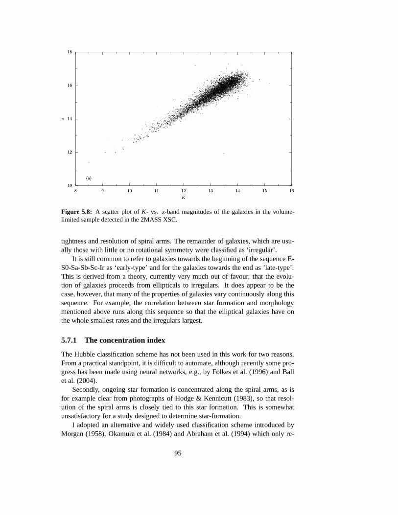
(a)(a)

1010

1212

1414

1616

1818

zz

88 99 1010 1111 1212 1313 1414 1515 1616

KK

Figure 5.8: A scatter plot of K- vs. z-band magnitudes of the galaxies in the volume-limited sample detected in the 2MASS XSC.

tightness and resolution of spiral arms. The remainder of galaxies, which are usu-ally those with little or no rotational symmetry were classified as ‘irregular’.

It is still common to refer to galaxies towards the beginning of the sequence E-S0-Sa-Sb-Sc-Ir as ‘early-type’ and for the galaxies towards the end as ’late-type’.This is derived from a theory, currently very much out of favour, that the evolu-tion of galaxies proceeds from ellipticals to irregulars. It does appear to be thecase, however, that many of the properties of galaxies vary continuously along thissequence. For example, the correlation between star formation and morphologymentioned above runs along this sequence so that the elliptical galaxies have onthe whole smallest rates and the irregulars largest.

5.7.1 The concentration index

The Hubble classification scheme has not been used in this work for two reasons.From a practical standpoint, it is difficult to automate, although recently some pro-gress has been made using neural networks, e.g., by Folkes et al. (1996) and Ballet al. (2004).

Secondly, ongoing star formation is concentrated along the spiral arms, as isfor example clear from photographs of Hodge & Kennicutt (1983), so that resol-ution of the spiral arms is closely tied to this star formation. This is somewhatunsatisfactory for a study designed to determine star-formation.

I adopted an alternative and widely used classification scheme introduced byMorgan (1958), Okamura et al. (1984) and Abraham et al. (1994) which only re-

95

lies on one parameter — the concentration index. The concentration index, C,is defined as the ratio of the Petrosian 50%- to 90%-light radii. In this study Iused the r-band photometry to calculate the concentration index as it both has thehighest signal to noise and is less affected by recent star formation than the shorter-wavelength bands.

In the following section I will outline why the concentration index discrimin-ates between elliptical and disk dominated galaxies. Shimasaku et al. (2001) andStrateva et al. (2001) show that concentration indices calculated from the SDSS aregood proxies for traditional classification by eye though with quite a large scatter.

5.7.2 Light profiles

Elliptical galaxy light profiles are well described by the law first introduced by deVaucouleurs (1948) (for an early paper in English, see de Vaucouleurs 1953) :

I(α) = Ie exp[−7.67(α1/4−1)

](5.12)

where α = r/re is the ‘reduced radius’ defined as the ratio of the radius to theradius containing half of the total light of the galaxy (‘effective radius’, denotedre), and Ie is the surface brightness at the effective radius. This empirical model forthe light profile describes accurately the observed light profiles for a wide range ofα , from at least 0.03 to 20 or so.

If the seeing and other observational effects are disregarded, it can easily beshown using numerical integration that the ‘true’ concentration index for galaxiesobeying this model is C = 0.18. The very extended nature of the de Vaucouleurs’profile (see Figure 5.9) in combination with photometry methods used in practicemeans that this is never the value actually measured. For Petrosian photometrythat I use, the concentration index of an idealised elliptical is C = 0.32. The ef-fect of seeing is to decrease the central concentration of light in galaxies, whichcorresponds to an increase in the numerical value of C.

The significance of seeing on the galaxy classification for the primary samplecan be estimated as follows. The typical seeing during SDSS imaging runs was1.′′4, which corresponds3 to about 1.8h−1 kpc at the far edge of the volume limitedsample (z = 0.1).

Elliptical galaxies show a wide range of effective radii from about 2 to 14 kpc(see, e.g., Kormendy, 1977); most, however, have re > 3kpc. In fact, Kormendy(1977) showed that re and the absolute galaxy magnitude in the blue, MB, satisfy arelationship which can be written as:

MB =−1.98log re + c, (5.13)

indicating, as may be intuitively expected, that the more luminous galaxies havelarger physical sizes. Given these results, and the typical seeing, it can be con-cluded that the concentration indices that are measured for early-type galaxies inthe volume limited sample are not dominated by the effects of seeing.

3I will later adopt h = 0.7, in which case this corresponds to 2.5kpc.

96

00

0.20.2

0.40.4

0.60.6

0.80.8

11

f(α

)f(α

)

00 22 44 66 88 1010

αα

Figure 5.9: Fraction of total light contained within reduced radius α for de Vaucouleurs’(solid line) and exponential (dashed line) profiles.

The typical distribution of light in galaxy disks is well described by an expo-nential law (see, e.g., Freeman, 1970):

I(α) = I0 exp(−α) (5.14)

where α is the dimensionless radius defined as radius divided by the characteristicscale. By appropriate integration it can be shown that the fraction of light, f (α),contained within reduced radius α is:

f (α) = 1− exp(−α)−α exp(−α). (5.15)

From this relation it can be deduced—if the practicalities of observations are againdisregarded—that the concentration index for disk galaxies is approximately C ≈0.43. The fraction of total light as a function of the reduced radius are comparedfor de Vaucouleurs and exponential models in Figure 5.9.

5.7.3 Concentration index properties of the volume-limited sample

The concentration indices of galaxies in the volume-limited sample were calculatedusing photometry supplied in the SDSS imaging catalogues. The resulting distri-bution of the concentration index for the non-AGN, z > 0.03, subsample is shownin Figure 5.10. As an illustration of the effectiveness of the concentration index todistinguish between the basic galaxy morphologies, the relationship between themean Hα equivalent width and concentration index is shown in Figure 5.11. It can

97

0.50.5

11

22

55

1010

2020

5050

100100

200200

500500

10001000

NN

0.250.25 0.30.3 0.350.35 0.40.4 0.450.45 0.50.5 0.550.55 0.60.6

CC

Figure 5.10: The distribution of concentration index values for galaxies in the volume-limited sample with z> 0.03 and which are not dominated by AGN.

be seen in the figure that there exists a tight correlation which reflects the correla-tion between Hubble type and Hα equivalent width as presented by, for example,Kennicutt (1998a) in his Figure 3.

98

00

2.52.5

55

7.57.5

1010

12.512.5

1515

17.517.5

EW

(Hα

)(A

)EW

(Hα

)(A

)

0.250.25 0.30.3 0.350.35 0.40.4 0.450.45 0.50.5

CC

Figure 5.11: The mean equivalent width of the Hα line as a function of the r-band con-centration index.

99

100

Chapter 6

A statistical study of the effects ofinteractions on galaxies:triggering of star formation

6.1 Finding nearest companions

To investigate the effects of pair-wise tidal interaction on galaxy properties onewould ideally like to know the nearest companion of significant mass to each ofthe galaxies in the sample and the physical separation to it. The separation pro-jected onto the plane of the sky is of course easily measured, but the line-of-sightcomponent is poorly constrained for the following reasons: peculiar velocities ofgalaxies produce errors in redshift-based distance estimation comparable to typicalseparations to the nearest companion (/ 1Mpc); and, even more importantly, evenwith a large scale comprehensive survey like the SDSS, the sample of galaxies withmeasured redshifts is too incomplete to reliable identify nearest companions to asample like the volume-limited sample I constructed.

There two main reasons why galaxies with spectroscopic follow-up are in-adequate for the identifying companions. The first is the minimum separationbetween spectroscopic fibres and the finite number of these fibres an any one plateboth of which mean that galaxies which are close together are unlikely to be bothobserved even if they satisfy selection criteria for the follow-up sample. This prob-lem is only partially alleviated in the overlap regions which belong to more thanone plate. The second reason are the follow-up selection criteria themselves, mostnotably the 17.7 limiting r-band magnitude. Since most of our volume limitedsample is within one magnitude of this cut-off (see Figure 6.1), companions selec-ted from the MGS will necessarily be required to be as luminous as the primarygalaxy.

In order to avoid these problems, candidate nearest companions were selectedfrom the photometric data. If a spectroscopic redshift is available for a particularcandidate it is used in deciding whether to accept or reject the candidate; however,

101

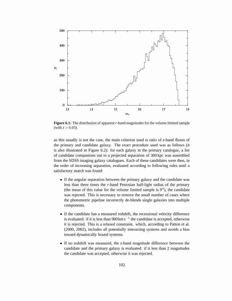
00

100100

200200

300300

400400

500500

NN

1313 1414 1515 1616 1717 1818

mrmr

Figure 6.1: The distribution of apparent r-band magnitudes for the volume limited sample(with z > 0.03).

as this usually is not the case, the main criterion used is ratio of z-band fluxes ofthe primary and candidate galaxy. The exact procedure used was as follows (itis also illustrated in Figure 6.2): for each galaxy in the primary catalogue, a listof candidate companions out to a projected separation of 300 kpc was assembledfrom the SDSS imaging galaxy catalogues. Each of these candidates were then, inthe order of increasing separation, evaluated according to following rules until asatisfactory match was found:

• If the angular separation between the primary galaxy and the candidate wasless than three times the r-band Petrosian half-light radius of the primary(the mean of this value for the volume limited sample is 9′′), the candidatewas rejected. This is necessary to remove the small number of cases wherethe photometric pipeline incorrectly de-blends single galaxies into multiplecomponents.

• If the candidate has a measured redshift, the recessional velocity differenceis evaluated: if it is less than 900km s−1 the candidate is accepted, otherwiseit is rejected. This is a relaxed constraint. which, according to Patton et al.(2000, 2002), includes all potentially interacting systems and avoids a biastoward dynamically bound systems.

• If no redshift was measured, the z-band magnitude difference between thecandidate and the primary galaxy is evaluated: if it less than 2 magnitudesthe candidate was accepted, otherwise it was rejected.

102

For each entry in Primary Catalogue

Select next closest candidate

Secure redshift?

∆zhelio < 0.003? ∆z < 2 mag

Found the closest pair θsep > 3 × Petr. half-light radius

Yes

YesY

es

No

Yes

No

No

No

1

Figure 6.2: Schematic representation of the algorithm used to select nearest companions.

This procedure resulted in 12492 of the 13973 galaxies in the volume limitedsample being identified with companions. Of these, 2038 have measured spectra,whilst the remaining systems have only imaging data. The resulting distribution ofthe separations to the identified companion is shown in Figure 6.3.

Completeness of the companions catalogue

The resulting catalogue is expected to be substantially complete for companionswithin the following well defined limits:

1. Projected separation greater than three times the half-light radius of theprimary galaxy. At the median redshift of the volume-limited sample andthe median half-light radius, this requirement corresponds to a minimumseparation of 14 kpc.

2. Projected separations smaller than 300 kpc. Only a small fraction of galaxieshave no companion withing this radius.

3. The mass ratio of the primary and companion (as traced by the z-band lu-minosity) is less than approximately six.

Requirement 1 effectively alleviates any problems with the de-blending al-gorithm while requirement 3 and the relatively bright limit of the volume limitedsample mean that almost all potential companions will have high signal to noise

103

00

0.0050.005

0.010.01

0.0150.015

0.020.02

ff

00 0.050.05 0.10.1 0.150.15 0.20.2 0.250.25 0.30.3 0.350.35

rp (Mpc)rp (Mpc)

Figure 6.3: Distribution of projected separations to the nearest companion.

detections in the imaging. The exception are very low surface-brightness galaxieswhich are difficult to identify in any imaging survey.

The above constraints must be borne in mind when interpreting the data; theimply that, by definition, no merging systems are identified as such; and, compan-ions less that one-sixth of the mass of the primary are not considered.

Projection Effect Pairs

Some of the companions selected in this way will in fact be interloping (or pro-jection effect) companions, which have large line-of-sight separations and are notphysically connected in any way with the primary galaxy.

Exact analysis of this problem requires consideration of the three-dimensionalclustering of galaxies as well as an exact definition of how big line-of-sight separa-tions can be tolerated. An approximate analysis can be carried out, much along thelines of that presented by Rose (1977), by considering the non-physically relatedgalaxies to be a random field. The probability that one of these physically unre-lated galaxies occurs within radius r of any point, which we take to coincide withthe primary galaxy, is given by:

P(r) = 1− exp(−r2πσ), (6.1)

where σ is the density of galaxies on the sky in the brightness range considered.In the present case, this range is 2 magnitudes brighter or fainter than the primarygalaxy, and for this reason the probability distribution will be different for each

104

0

0.2

0.4

0.6

0.8

1

Pro

bab

ility

ofpro

ject

ion

pai

r

0 0.05 0.1 0.15 0.2 0.25 0.3 0.35

Pair Separation (Mpc)

Figure 6.4: Mean probability of a non-physical pair as a function of separation from theprimary galaxy.

primary galaxy. The density of galaxies for any particular range of brightness iseasily calculated using the parametrised z-band SDSS galaxy counts:

N(z-mag < m) =13

deg2 ×100.6(m−16). (6.2)

as derived by Yasuda et al. (2001).The chance of an interloping pair is summarised in Figure 6.4, which shows the

mean of P(r) over the volume-limited sample. It is clear that projection effect pairsbecome significant at separations of around 150 kpc. Therefore, some care needs tobe exercised when interpreting results at these and larger separations. At the sametime, it should also be noted that, within the limits mentioned above, the separationto the nearest companion, even it is due to a projection effect, is a reliable a lowerlimit to the separation to the true nearest companion. It is also worth noting thatthe projection pairs effectively limit the range of primary/companion mass rangesthat can be probed using this photometric technique.

6.2 Results

The observed relationship between the mean specific star-formation rate and pro-jected separation to the nearest companion is shown in Figure 6.5. The galaxiesfor this figure were drawn from the volume-limited sample with an additional red-shift constraint z > 0.03 and were split into three concentration index bins corres-

105

00

5 · 10−115 · 10−11

1 · 10−101 · 10−10

1.5 · 10−101.5 · 10−10

2 · 10−102 · 10−10

2.5 · 10−102.5 · 10−10

ψm

(yr−

1)

ψm

(yr−

1)

00 0.050.05 0.10.1 0.150.15 0.20.2 0.250.25 0.30.3

Pair Separation (Mpc)Pair Separation (Mpc)

Figure 6.5: Mean normalised star formation rate as a function of separation to the nearestcompanion for galaxies in the volume-limited sample. Open circles: late-type galaxies(C > 0.375); open diamonds: mixed-type galaxies (0.33 < C ≤ 0.375); filled squares:early-type galaxies (C ≤ 0.33).

ponding approximately to late-, mixed-, and early-type morphologies. The specificstar-formation rate was derived from Hα luminosity calculated as described in Sec-tion 5.4 and converted using the relation in Section 2.2.

The bin size used for this and most of the following figures is 10 kpc below100 kpc and 40 kpc thereafter. The error bars show estimated random errors onthe mean of each bin, as calculated from standard deviation of data within eachbin; they are dominated by the intrinsic variance of the sample rather than randomerrors in measurement of the Hα flux.

As a way of displaying this relationship without any binning, I have calculatedand plotted on the same figure as a broken line the function of the form:

ψm(rp) = a1

(rp

25kpc

)β1

+ a2

(rp

25kpc

)β2

, (6.3)

that best fits (in the simple χ 2 sense) the individual data points of each morpholo-gical bin. The corresponding best-fitting parameters are shown in Table 6.1.

The effect of the finite fibre aperture and the correction I applied for this cannot be exactly quantified without a comprehensive spatially resolved survey of Hαemission. The variation of apparent angular size of galaxies with redshift can, how-ever, be used to explore this problem as, clearly, the higher redshift galaxies requireless correction. This can be seen in Figure 6.6 in which the late-type sub-sampleis split into two redshift bins and both the aperture corrected and non-correctedstar-formation rates are plotted as functions of separation to nearest companion.

106

(a)(a)

00

2 · 10−112 · 10−11

4 · 10−114 · 10−11

6 · 10−116 · 10−11

8 · 10−118 · 10−11

ψm

(yr−

1)

ψm

(yr−

1)

00 0.050.05 0.10.1 0.150.15 0.20.2 0.250.25 0.30.3

Pair Separation (Mpc)Pair Separation (Mpc)

(b)(b)

00

1 · 10−101 · 10−10

2 · 10−102 · 10−10

3 · 10−103 · 10−10

4 · 10−104 · 10−10

ψm

(yr−

1)

ψm

(yr−

1)

00 0.050.05 0.10.1 0.150.15 0.20.2 0.250.25 0.30.3

Pair Separation (Mpc)Pair Separation (Mpc)

Figure 6.6: Comparison of (a) non-aperture corrected and (b) aperture-corrected star-formation rates versus separation for late-type galaxies in two redshift bins: 0.03 < z ≤0.07 (open circles) and 0.07< z≤ 0.1 (full squares).

107

Table 6.1: The dependence of the specific star formation rate on projec-ted separation is characterised by fitting a two power-law function to thespecific star formation rate vs pair separation data (Fig. 6.5) after its beendivided according to morphological type.

Concentration a1 β1 a2 β2

Index bin (10−11 yr−1) (10−11 yr−1)

0<C ≤ 0.33 2.0 −0.5 0.1 1.20.33 <C ≤ 0.375 6.3 −0.4 0.7 0.70.375 <C ≤ 1.0 14 0.0 2.9 −1.0

It is clear from this figure that the non-corrected and corrected data exhibit asimilar trend with pair separation. The non-corrected data, however, show a markeddifference between the two redshift bins, indicating that the Hα luminosity is sig-nificantly underestimated without aperture correction. The corrected data bring thetwo redshift bins in surprisingly good agreement, although the discrepancy at closeseparations is indicative of a small overcorrection for these systems. The implic-ation of this is that galaxies with close companions have star formation which isenhanced in the nuclear region compared to the periphery – that is, they harbournuclear starbursts. Therefore, although the over-estimate of aperture correction forclose pairs contributes to the uncertainty in our measurement of enhancement ofstar formation in those pairs, the existence of this over-correction is in itself strongevidence of nuclear starbursts in galaxies with close companions.

For the subsample of galaxies detected in the IRAS all-sky survey I was ableto contrast in Figure 6.7 the dependence of far-infrared derived (Section 5.4.4) andHα derived star formation rates on pair separation. In order to take into accountthe possibility that both the primary galaxy and its companion are contributingto the measured far-infrared fluxes, two mass normalisations of the FIR-derivedstar-formation rates are shown in the figure: normalisation by mass of the primarygalaxy (as I used everywhere else, open diamonds); and, normalisation by the sumof the masses of primary and companion galaxies if their separation is less than 1.5arcminutes, and just the primary mass otherwise (solid squares on the plot).

The comparison is limited to those systems for which both FIR and Hα areavailable so this is inevitably biased towards systems with higher star formationrates. However, these are precisely the systems in which any problems associatedwith the use of Hα as a star-formation rate estimator are likely to be the greatest.I find good agreement between the FIR, especially when normalised to the sum ofthe masses of the primary and companion galaxies, and Hα data both in terms ofthe trend with projected pair separation and the magnitude of the specific star form-ation rate. I conclude that the procedure used here to estimate the star-formationrate from Hα data gives a good and predominantly unbiased estimate of the true

108

00

2 · 10−102 · 10−10

4 · 10−104 · 10−10

6 · 10−106 · 10−10

8 · 10−108 · 10−10

1 · 10−91 · 10−9

ψm

(yr−

1)

ψm

(yr−

1)

00 0.050.05 0.10.1 0.150.15 0.20.2 0.250.25 0.30.3

Pair Separation (Mpc)Pair Separation (Mpc)

Figure 6.7: Specific star-formation rates for galaxies detected by IRAS; open circles: Hαstar-formation estimator (as before); open diamonds: FIR star-formation estimator; solidsquares: FIR star-formation estimator but normalised by mass of both the primary andcompanion galaxies if they are within 1.5 arcminutes of each other.

star-formation rate.It is clear from both the means of the binned data and the best-fitting curves

shown in Figures 6.5 and 6.7 that there is an enhancement of specific star-formationrates of galaxies with companions closer than approximately 50 kpc. This en-hancement is further investigated in Figure 6.8 where I contrast the distributionsof specific star-formation rates for galaxies with companions closer than 50 kpcand further than 200 kpc. The Kolmogorov-Smirnov (K-S) test indicates, at a sig-nificance level greater than 99.9%, that the these two distributions are drawn fromdifferent parent distributions confirming that galaxies with close companions havesignificantly different specific star-formation rates.

On properties of enhancement of star formation

Having established enhancement of star formation for galaxies with close compan-ions I now briefly consider the properties of this enhancement by examining whattypes of galaxies show the greatest enhancement. In Figure 6.9, the relationshipbetween pair separation and specific star formation is shown for three subsamplesof galaxies selected according to their (non-specific) star-formation rates. It isclear from this figure that the observed increase of star-formation at r p < 50kpccan be attributed to galaxies with star-formation rates greater than 3 M� yr−1 andthat galaxies with star-formation rates greater than 10 M�yr−1 show the greatestfactional and absolute enhancement.

109

10−410−4

10−310−3

10−210−2

10−110−1

100100

ff

00 2.5 · 10−102.5 · 10−10 5 · 10−105 · 10−10 7.5 · 10−107.5 · 10−10 1 · 10−91 · 10−9 1.25 · 10−91.25 · 10−9

ψm (yr−1)ψm (yr−1)

rp < 50 kpcrp < 50 kpc

rp ≥ 200 kpcrp ≥ 200 kpc

Figure 6.8: The relative distribution of specific star-formation rates for galaxies from thelate-type volume limited sample with close companions (solid line) and no companions orcompanions which are separated by more than 200 kpc (dashed line).

00

2 · 10−102 · 10−10

4 · 10−104 · 10−10

6 · 10−106 · 10−10

8 · 10−108 · 10−10

1 · 10−91 · 10−9

ψm

(yr−

1)

ψm

(yr−

1)

00 0.050.05 0.10.1 0.150.15 0.20.2 0.250.25 0.30.3

Pair Separation (Mpc)Pair Separation (Mpc)

Figure 6.9: Specific star formation versus projected separation to nearest companion forthree sub-samples selected from the late-type sample according to absolute star formationrate: 0< ψ < 3M� yr−1 , 3M� yr−1 < ψ < 10M� yr−1 and ψ > 10M�yr−1.

110

Table 6.2: Parameters obtained when fitting a two power-law function to plots ofspecific star formation rate as a function of pair separation for three sub-samplesof systems, selected according to SFR.

SFR range (M� yr−1) a1 (yr−1) β1 a2 (yr−1) β2

0< ψ ≤ 3 3.26×10−11 −0.10 2.98×10−11 −0.093 < ψ ≤ 10 1.40×10−10 −0.10 1.14×10−10 −0.10

10 < ψ ≤ 1000 1.43×10−10 −1.37 4.03×10−10 0.05

Light profiles

The approximately factor of ten difference between mean specific star-formationrates of galaxies with C < 0.33 and C > 0.375 that can be seen in Figure 6.5 isan illustration of the power of the concentration index to discriminate between latetype, gas rich, and early type, normally gas poor, galaxies. The index is, however,a relatively simple measure based on single colour data and will have limitations.

Our investigations of these limitations led us to consider the relation betweenthe concentration index and separation to nearest companion, which is shown inFigure 6.10. A surprisingly tight relationship can be seen: galaxies with com-panions closer than 50 kpc are significantly more centrally concentrated than thosewith companions in the range 50kpc < rp < 250kpc; at separations greater thanabout 250 kpc there appears to be another drop in concentration index although thestatistical significance of this has not been definitely established. The implicationsof these findings are discussed later.

Star formation properties as a function of recessional velocity separation

In approximately one-fifth of our volume limited sample the companion galaxyhas a measured SDSS spectrum, and therefore, in essentially all cases, a measuredredshift. In Figure 6.11 I examine the effect of the recessional velocity differenceon star formation rate for these galaxies. The best-fitting parameters from fittinga two power-law model are shown in Table 6.3. The data reveal a decline in thespecific star-formation rate with increasing recessional velocity difference out to900kms−1. The magnitude of this effect is smaller than that observed betweenspecific star-formation rate and projected separation. The steepest decline is seenat small velocity differences.

A correlation between projected separation and velocity difference may be ex-pected if, for example, all systems were bound. I find no correlation between thesetwo quantities for this sample; the mean velocity separation is ∼ 200km s−1 and isindependent of projected separation.

111

0.370.37

0.380.38

0.390.39

0.40.4

0.410.41

CC

00 0.050.05 0.10.1 0.150.15 0.20.2 0.250.25 0.30.3

Pair Separation (Mpc)Pair Separation (Mpc)

Figure 6.10: Mean r-band concentration index as a function of separation to the nearestcompanion. The dashed line is the least-squares best-fitting function of the form C =a1(rp/25kpc)β1 + a2(rp/25kpc)β2 ; the best fit parameters are: a1 = 1.6, β1 = 0.19, a2 =−1.20, and β2 = 0.24.

00

5 · 10−115 · 10−11

1 · 10−101 · 10−10

1.5 · 10−101.5 · 10−10

2 · 10−102 · 10−10

2.5 · 10−102.5 · 10−10

ψm

(yr−

1)

ψm

(yr−

1)

00 200200 400400 600600 800800

Velocity difference (km s−1)Velocity difference (km s−1)

Figure 6.11: Specific star-formation rate of late type galaxies (C > 0.375) as a function ofvelocity separation.

112

Table 6.3: Parameters obtained when fitting a twopower-law function to the plot of specific star form-ation rate as a function of the recessional velocity ofspectroscopic galaxy pairs.

a1 (yr−1) β1 a2 (yr−1) β2

4.56×10−10 0.05 1.43×10−10 −1.38

11

1010

100100

10001000

NN

00 2.5 · 10−102.5 · 10−10 5 · 10−105 · 10−10 7.5 · 10−107.5 · 10−10 1 · 10−91 · 10−9 1.25 · 10−91.25 · 10−9

ψm (yr−1)ψm (yr−1)

latelate

mixedmixed

earlyearly

Figure 6.12: Distribution of specific star formation rates for galaxies with companionscloser than 50 kpc, split according to the morphological type of the companion.

6.2.1 Dependence on the properties of the interaction

We do not expect all tidal interactions to lead to enhanced star formation. Howeffective a given interaction is at triggering gas inflow etc. may depend not onlyon the properties of the perturbed galaxy (which we have examined in the previoussection), but also upon the nature of the perturber. The nature of the perturbinggalaxy can be probed in two ways: its morphological class and mass.

In Figure 6.12 I show the distribution of specific star-formation rates for late-type galaxies with a companion within 50 kpc. I split the pairs into three sub-samples depending on the morphological type of the perturber: late-late, late-mixed and late-early pairs. There are no significant differences between thesesub-samples: the Kolmogorov-Smirnov (K-S) test applied between the late-lateand late-early distributions gives a formal significance of only 20% that they aredrawn from different distributions.

113

11

1010

100100

10001000

NN

00 2.5 · 10−102.5 · 10−10 5 · 10−105 · 10−10 7.5 · 10−107.5 · 10−10 1 · 10−91 · 10−9 1.25 · 10−91.25 · 10−9

ψm (yr−1)ψm (yr−1)

−2 < ∆mz ≤ −1−2 < ∆mz ≤ −1

−1 < ∆mz ≤ 0−1 < ∆mz ≤ 0

0 < ∆mz ≤ 20 < ∆mz ≤ 2

Figure 6.13: Distribution of specific star formation rates for galaxies with pairs closer than50 kpc, split according to z-band magnitude difference.

I investigate the effect of companion mass in Figure 6.13. Again, I split thosesystems which have companions with projected separations less than 50 kpc intothree sub-samples according to the z-band magnitude difference between the pri-mary and companion galaxy [∆mz = mz(primary)−mz(companion)]. For all spe-cific star-formation rates I find an excess of systems where the companion is oflower mass than the primary galaxy. This effect is mainly due to form of the lumin-osity function which rises steeply to lower luminosities at the limit of our primarysample. Therefore, for real physical pairs, a galaxy of a given luminosity is morelikely to be interacting with a galaxy of lower luminosity. I have used the K-S testto compare the SSFR of the three subsamples. I tested the null hypothesis that thethree distributions are all drawn from the same parent distribution. I find no evid-ence to reject the null hypothesis – the formal confidence level that the distributionsare drawn from different populations is 50%.

6.3 Discussion

6.3.1 Potential biases

Aperture and extinction correction

The method used to estimate star-formation rates for our sample follows closelythat used by Hopkins et al. (2003), who have done extensive comparisons of thismethod to radio and far-infrared estimators and found good agreement. Because

114

the method employed is based on the assumption of constant Hα equivalent widthacross the galaxy, it will significantly contribute to errors in individual objects. Forexample, for systems in which star formation is concentrated in the nucleus it willoverestimate the total star-formation rate. On the other hand, if the majority of starformation is off-nuclear, or if the fibre is not accurately positioned on the nucleus,then the aperture correction will not recover the true star-formation rate.

The data presented in Figure 6.6 demonstrate quite clearly the benefits of aper-ture correction. They also indicate that there may be a small over-estimate for thelower redshift systems with close companions. This over-estimate is, however, initself evidence for triggering of nuclear star-bursts in these systems. Furthermore,the similarity of far-infrared and Hα derived star-formation rates shown in Fig-ure 6.7 makes it unlikely there are any significant biases which could affect theinterpretation of these data.

Dwarf galaxies

The pair selection algorithm described above only considers companion galaxiesif they are further than three times the Petrosian half-light radius of the primarygalaxy. For this reason, it is reasonable to expect that galaxies with intrinsicallysmaller half-light radii will dominate the very shortest separations. If these galaxieswere dwarf galaxies, there would be a potential bias since dwarf galaxies havehigher specific star-formation rates than spiral galaxies.

This possibility is easily rejected by examining the relative proportion of dwarfgalaxies we would expect in our volume and luminosity limited sample. Using theluminosity functions presented by Schwarzkopf & Dettmar (2000) it can easily beshown that the total number of dwarf galaxies in our sample is at most 0.5 per-cent,with about one-tenth of those being dwarf irregulars and the rest dwarf spheroidalgalaxies.

Systematic errors in galaxy mass estimates

Because I generally use specific star-formation rates in this investigation, there isa possibility that a systematic underestimate of galaxy masses (see Section 5.6)could lead to us to wrong conclusions; for example, if galaxy masses are system-atically underestimated at close separations, this would appear as an enhancementof the specific star-formation rate and therefore could be interpret as evidence fortriggered star formation.

One possibility which was considered was that dust obscuration is higher ingalaxies with close companions. This can be tested by repeating the comparisonbetween K and z magnitudes for only galaxies with close companions. Our res-ults indicate that the dispersion around proportionality for these galaxies is 0.27magnitudes, negligibly larger than the 0.25 dispersion of the whole sample.

The other possibility considered was that galaxies with close companions willhave, as a result of tidal forces, light distributions with a greater proportion of light

115

in low-surface brightness features which will not be picked up by the photometry.This seems unlikely because Schwarzkopf & Dettmar (2000) show, although for asample of limited size, that galaxy light profiles are not significantly extended ininteracting galaxies. In addition, the Petrosian photometry I use does not employa fixed limiting magnitude, but rather depends on the overall shape of the profile(see Section 5.6.1 and Strauss et al. 2002).

6.3.2 Triggering of star formation

I find that star formation in galaxies with companions at projected separations lessthat 50 kpc is significantly enhanced compared to galaxies with companions at lar-ger separations. This finding is similar to those obtained by Barton et al. (2000)and Lambas et al. (2003) for smaller samples and different analysis techniques.

Using the best-fitting curve published by Lambas et al. (2003) it is possible toquantitatively compare their and our results. The functional form used to fit thedata in Lambas et al. (2003) is a single power-law of the form 〈b〉 = a1rβ

p where bis the birth parameter defined as:

b = Ψ/Ψ, (6.4)

and Ψ is the time averaged star-formation rate. For a particular star formationhistory, this birth parameter is proportional to ψm and so, to first order, we candirectly compare these two. I have fitted my data using a similar functional formand restricting the range of projected separations to that used by Lambas et al.(2003) [0< rp < 100×(0.7)−1 kpc]. After converting results to a common distancescale, it was found that I measure a smaller magnitude of triggering than Lambaset al. (2003). The results presented here can, however, be reconciled with thoseof Lambas et al. (2003) if an additional constraint ψm > 2×10−11 yr−1 is applied.This is interpreted as evidence of bias towards star-forming systems in the sampleused by Lambas et al. (2003).

Although our results are limited to a relatively small sub-sample that has beendetected by IRAS, I find that enhanced star formation in galaxies with close com-panions manifests itself with equal magnitude in optical spectra and far-infraredcontinuum. The invariance of the observed results under the completely differentsystematics that influence these techniques lend considerable weight to our inter-pretations.

Because the separation between the primary and companion galaxies in oursample is often comparable to or smaller than the size of the IRAS beam, thereis a possibility that both of these galaxies contribute to the measured far-infraredflux. As a first order approximation, it is not unreasonable to disregard this possib-ility, as I have done for one of the results presented in Figure 6.7. The reason whythis reasonable is that Surace et al. (2004) find that when far-infrared emission ofinteracting galaxies can be resolved with IRAS only one of the two galaxies is usu-ally luminous; more precisely, the ratio of infrared luminosities of the component

116

galaxies is greater than three in two-thirds of cases. Under this approximation thereis, however, a significant discrepancy at close separations between far-infrared de-rived and Hα derived specific star formation rates. This may then be an indicationthat we underestimate extinction in galaxies with close companions systems.

Our second approach takes into account the possibility that both the primaryand companion galaxies are contributing significantly the IRAS far-infrared fluxesby normalising the derived star-formation rate by the sum of the z-band derivedstellar masses. This effectively means that we calculate the mean of specific star-formation rates of the two galaxies. I find that this method produces specific star-formation rates which are in excellent agreement with those derived from Hαdata. These results therefore suggest that members of interacting systems havefar-infrared luminosities approximately in proportion to their stellar masses.

6.3.3 Light profiles of interacting galaxies

I have discovered a tight relationship—shown in Figure 6.10—between the con-centration index and projected separation to the nearest companion. A particularlystriking feature of this relationship is the rapid and highly significant decline of themean concentration index at projected companion separations smaller than 50 kpc.Additionally, there appears to be a decline with increasing separation between100 kpc and 300 kpc. The importance of projection-effect pairs at these separa-tions however means that this second result must be treated with caution.

This result can be interpreted in several ways: for example, it may simplybe a consequence of the morphology-density relationship discovered by Dressler(1980); or, it may be due to redistribution of stellar content of galaxies by tidalforces, e.g., by disrupting the outer parts of the disk onto a more extended structure.

Although the density-morphology relationship is an attractive candidate to ex-plain the decline at close separations, further investigation has shown that it isunlikely to be to a significant factor. Firstly, direct investigation of how the densityof environment depends on companion separation does not reveal any systematicchange over the range 0< rp < 100kpc (Section 7.3.2). Secondly, the length-scaleat which decline occurs (≈ 50kpc) is much smaller than the characteristic lengthscales associated with clusters (≈ 1Mpc). Finally, the fraction of galaxies in verydense environments such as clusters is small—the value given by Dressler (1984)is 5 percent—and therefore it is unlikely they would influence the properties of thewhole sample.

The second possibility, that tidal forces cause on average significant transfer ofstellar material outwards, has already been touched upon in Section 6.3.1. Furtherinvestigation has shown that the decline at close separation is not a consequence ofexpansion of the 90%-light radius and that therefore, this mechanism is unlikely tobe the cause of the observed effect.

Our favoured interpretation of the sharp decline of the concentration index ofgalaxies with companions at close separations is that it is due to triggering of nuc-lear starbursts. The resulting young and luminous stars make the galaxy light ap-

117

pear significantly more concentrated even though the distribution of galaxy massis essentially unchanged. Under this interpretation of the results, the observedscale at which the turnover of mean concentration index occurs—i.e., approxim-ately 50 kpc—is a good indication of the physical scales at which tidal interactionsbegin to drive nuclear starbursts.

Such an interpretation would also be consistent with the data shown in Fig-ure 6.6, which suggest that the equivalent width of the Hα line is more stronglyenhanced in nuclear regions, as well as previous studies, such as that by Keel et al.(1985), which find that the induced activity tends to be concentrated in the nuclei.

If nuclear star bursts are indeed the cause of the concentration index-companionseparation relation it is clear the concentration index too suffers from one of thedrawbacks of the Hubble classification scheme, namely it is sensitive to star form-ation. Some care therefore need be exercised when interpreting our results, par-ticularly at rp < 50kpc where the mean concentration index varies rapidly withcompanion separation. For example, it is possible that some or even all of theenhancement of SSFR in mixed- and early-type galaxies with close companionsmay in fact be due to mis-classification in the sense that galaxies with strong diskcomponents are classified as early types because of unclear star-bursts and con-sequently placed in the earlier bins.

6.3.4 What controls star formation in galaxies?

It is immediately clear from Figure 6.5, as well as from the relation shown inFigure 5.11, that galaxy morphology as traced by the concentration index playsan important and possibly dominant role determining star-formation properties ofgalaxies. As the processes which give rise to observed galaxy morphologies arenot currently understood it is difficult to establish the precise nature of the linkbetween morphology and star formation. On a simple level however, the observedrelationship can be explained as a consequence of the large difference along themorphological sequence in the content of atomic and molecular hydrogen.

In this work it has been established, beyond reasonable doubt, that galaxy-galaxy interactions also play a role in controlling star formation. On the projectedseparation scales that have been probed, rp' 15kpc, the mean effect of interactionsis minor compared to the effects of morphology; for example, the mean SSFR ofmixed-type galaxies in closest pairs that I find is smaller than the mean SSFRof most widely separated galaxies in the late-type morphological bin. Also theabsolute increase in SSFR at close separations is smaller for early- and mixed-typegalaxies compared to late-types.

These findings point towards the importance of a ready supply of relativelycool gas in fuelling star formation. It seems unlikely that interactions generatethis supply through, for example, accretion of gas—consistent with the finding thatmorphology of the companion does not plays a significant part in triggering ofstar-formation. The view of interactions that emerges is one consistent with theresults of numerical simulations: they provide a mechanism for dissipation of gas

118

energy and angular momentum leading to enhanced star formation, much of whichis concentrated in the nuclear region.

The large population variance within each separation bin suggests that there areother factors besides morphology and projected separation which are important.Obvious candidates are the interaction orbit parameters, such the relative orienta-tion of the spin vector of the galaxy and angular momentum vector of the interact-ing system. These are, however, difficult to constrain without further observations.

Star formation in the important regime of strong interaction and merging (r p /15kpc) is not constrained by this study. Numerical simulations of Mihos & Hern-quist (1996) indicate that these end-stage interactions can rapidly convert availablegas into stars—consistent with observations of ULIRGs—and that the factor limit-ing the size of the resulting starburst is the fraction of gas that did not collapse intostars before the final merger. The current limit of approximately 15 kpc could besignificantly reduced by making use of deep, high-resolution, near-infrared ima-ging which makes identification of multiple nuclei significantly easier.

It is an inevitable consequence of the companion-identification algorithm usedthat what are in fact late-stage mergers are assigned a whole range of companionseparations. These will probably cause the star-formation in isolated systems tobe over-estimated leading, in turn, to an underestimate of the enhancement due tointeractions.

119

120

Chapter 7

A statistical study of the effects ofinteractions on galaxies: the roleof environment and what do thehigher ionisation lines tell us?

7.1 The influence of large scale environment on galaxies

The distribution of galaxies in space is far from uniform: there is strong clusteringand other structures on a wide range of scales (e.g., Tegmark et al., 2004). The‘environment’ of a galaxy, that is the space distribution other galaxies around it,can be most simply quantified in terms of the density of these galaxies measuredat some appropriate scale. It was first demonstrated by Dressler (1980) that in-ternal properties of galaxies show a very strong correlation with their environment:he showed that in nearby clusters there exists a tight relationship between galaxymorphology and local galaxy density, in the sense that early-type galaxies are moreprevalent in dense environments and late types in less dense environments. Gotoet al. (2003) expanded on this finding by showing that this density-morphologyrelationship continues to hold outside cluster environments and that the r-bandconcentration index is an adequate proxy for galaxy morphology for these studies.

Many of the other galaxy properties that have a strong dependence on environ-ment include:

• Integrated colour: galaxies are on average redder in dense environmentsBlanton et al. (2003a).

• Luminosity: galaxies are more luminous in dense environments (Kauffmannet al., 2004).

• Stellar mass: galaxies have larger stellar masses in dense environments (Kauff-mann et al., 2004).

121

• Star-formation rate: galaxies in less dense environments have a higher star-formation rates (e.g., Gomez et al., 2003).

• Dust content: Kauffmann et al. (2004) show that although low-mass galaxiesgenerally have the same dust content regardless of environment, the dustcontent of high-mass galaxies shows a strong dependence on environmentwith galaxies in less dense environment having more dust.

Almost all of the properties just listed also correlate between themselves (e.g.,Brinchmann et al., 2004); disentangling these correlations and working out thecausal relationships which lead to them is a topic of considerable importance forour understanding of galaxies and their evolution.

Recent evidence derived from large redshift surveys (mainly the SDSS) showsthat all of these correlations are not just the consequence of the density-morphologyrelationship. For example, Gomez et al. (2003) show that there exists a density-starformation relationship even when only galaxies of similar morphological type areconsidered. Additionally, Kauffmann et al. (2004) show that stellar mass plays animportant role of many of the correlations with environment while Blanton et al.(2003a) show that it is galaxy colours (and hence, star-formation histories) thatcorrelate most strongly with density of environment.

In this section, I investigate the connection between tidal interactions of galax-ies and the correlation between density and star-formation rates. Such a connec-tion is often invoked to explain the observed correlations of galaxy proprieties withdensity (e.g., Gnedin, 2003, and references therein) as, in a simple-minded pictureat least, interactions are more likely in the more dense environments. That this isin fact the case is not clear, and will be touched upon below.

The focus of this study is different from previous works which have beenprimarily concerned with tidal interaction as a mechanism for the hypotheticaltransformation of spiral to elliptical galaxies, postulated in order to explain thedensity-morphology relation. Here, I consider a different question, namely: Couldtidal interactions of galaxies in the field be responsible for the residual density-SFRrelationship even when the density-morphology relation is taken into account?

7.2 Measuring density of environment

The algorithm used to quantify the density of the environment is similar to thatused by Dressler (1980) in his original study of the relationship between densityand morphology: it is based on finding the projected separation to the n-th nearestneighbour, rn. This distance can, if required, be used to estimate the surface densityof galaxies via ΣD,n = n/r2

nπ .Unlike the original algorithm, the one presently employed makes use of the

measured redshifts of galaxies to search for nearest neighbours only in the red-shift shell ∆v =±1200km s−1 around the galaxy being considered (following Gotoet al., 2003, although our maximum velocity difference is slightly larger). Because

122

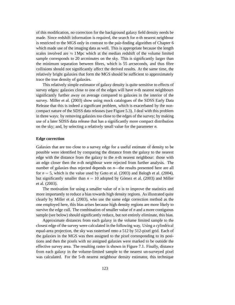
of this modification, no correction for the background galaxy field density needs bemade. Since redshift information is required, the search for n-th nearest neighbouris restricted to the MGS only in contrast to the pair-finding algorithm of Chapter 6which made use of the imaging data as well. This is appropriate because the lengthscales involved are ≈ 1Mpc which at the median redshift of the volume limitedsample corresponds to 20 arcminutes on the sky. This is significantly larger thanthe minimum separation between fibres, which is 55 arcseconds, and thus fibrecollisions should not significantly affect the derived results. At the same time, therelatively bright galaxies that form the MGS should be sufficient to approximatelytrace the true density of galaxies.

This relatively simple estimator of galaxy density is quite sensitive to effects ofsurvey edges: galaxies close to one of the edges will have n-th nearest neighbourssignificantly further away on average compared to galaxies in the interior of thesurvey. Miller et al. (2003) show using mock catalogues of the SDSS Early DataRelease that this is indeed a significant problem, which is exacerbated by the non-compact nature of the SDSS data releases (see Figure 5.3). I deal with this problemin three ways: by removing galaxies too close to the edges of the survey; by makinguse of a later SDSS data release that has a significantly more compact distributionon the sky; and, by selecting a relatively small value for the parameter n.

Edge correction

Galaxies that are too close to a survey edge for a useful estimate of density to bepossible were identified by comparing the distance from the galaxy to the nearestedge with the distance from the galaxy to the n-th nearest neighbour: those withan edge closer then the n-th neighbour were rejected from further analysis. Thenumber of galaxies thus rejected depends on n—the results presented here are allfor n = 5, which is the value used by Goto et al. (2003) and Balogh et al. (2004),but significantly smaller than n = 10 adopted by Gomez et al. (2003) and Milleret al. (2003).

The motivation for using a smaller value of n is to improve the statistics andmore importantly to reduce a bias towards high density regions. As illustrated quiteclearly by Miller et al. (2003), who use the same edge correction method as theone employed here, this bias arises because high density regions are more likely tosurvive the edge cull. The combination of smaller value of n and a more contiguoussample (see below) should significantly reduce, but not entirely eliminate, this bias.

Approximate distances from each galaxy in the volume limited sample to theclosest edge of the survey were calculated in the following way. Using a cylindricalequal-area projection, the sky was rasterised onto a 512 by 512-pixel grid. Each ofthe galaxies in the MGS was then assigned to the pixel corresponding to its posi-tions and then the pixels with no assigned galaxies were marked to be outside theeffective survey area. The resulting raster is shown in Figure 7.1. Finally, distancefrom each galaxy in the volume-limited sample to the nearest un-surveyed pixelwas calculated. For the 5-th nearest neighbour density estimator, this technique

123

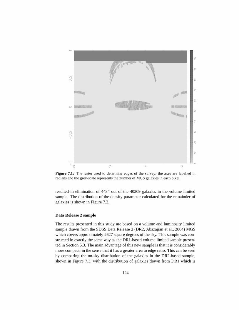
Figure 7.1: The raster used to determine edges of the survey; the axes are labelled inradians and the grey-scale represents the number of MGS galaxies in each pixel.

resulted in elimination of 4434 out of the 40209 galaxies in the volume limitedsample. The distribution of the density parameter calculated for the remainder ofgalaxies is shown in Figure 7.2.

Data Release 2 sample

The results presented in this study are based on a volume and luminosity limitedsample drawn from the SDSS Data Release 2 (DR2, Abazajian et al., 2004) MGSwhich covers approximately 2627 square degrees of the sky. This sample was con-structed in exactly the same way as the DR1-based volume limited sample presen-ted in Section 5.3. The main advantage of this new sample is that it is considerablymore compact, in the sense that it has a greater area to edge ratio. This can be seenby comparing the on-sky distribution of the galaxies in the DR2-based sample,shown in Figure 7.3, with the distribution of galaxies drawn from DR1 which is

124

100100

101101

102102

103103

104104

NN

0.50.5 11 22 55 1010

1/r5 (Mpc−1)1/r5 (Mpc−1)

Figure 7.2: Distribution of the density parameter 1/r5 in the volume limited sample.

shown in Figure 5.3. Additionally, the statistics are improved by the greater areaof the sky covered by DR2.

7.3 Results

Using the volume and luminosity limited sample, the data derived in Chapter 5and the densities derived using the method just described, I have re-derived themorphology-density (Dressler, 1980; Goto et al., 2003) and SFR-density (Gomezet al., 2003) relations. The larger and more compact area covered by DR2 improveson the statistics of previously published works but the trends are essentially thesame.

These correlations, which are shown in Figures 7.4 and 7.5 are striking bothbecause of their tightness and because of the great similarity between them. It canbe seen that both of the correlations extend over the full range of densities that arereliably sampled.

7.3.1 Can the density-morphology relation and tidal triggering ex-plain the density-SSFR relation?

As has already been mentioned, Gomez et al. (2003) found that there exists adensity-star formation correlation over and above what is likely to be due to thedensity-morphology relationship alone. This result is illustrated in Figure 7.6,where the mean specific star-formation rate of galaxies in narrow concentration

125

Figure 7.3: Hammer-Aitoff equal-area projection of galaxies in the primary volume-limited sample drawn from data release 2 of the SDSS.

126

0.330.33

0.340.34

0.350.35

0.360.36

0.370.37

0.380.38

0.390.39CC

0.50.5 11 22 55 1010

1/r5 (Mpc−1)1/r5 (Mpc−1)

Figure 7.4: Mean r-band concentration index as a function of density of environment forall of the volume limited sample drawn from DR2.

00

5 · 10−125 · 10−12

1 · 10−111 · 10−11

1.5 · 10−111.5 · 10−11

2 · 10−112 · 10−11

2.5 · 10−112.5 · 10−11

ψm

(yr−

1)

ψm

(yr−

1)

0.50.5 11 22 55 1010

1/r5 (Mpc−1)1/r5 (Mpc−1)

Figure 7.5: Specific star formation as a function of local density for non-AGN galaxies inthe redshift interval 0.03< z < 0.1 drawn from the volume limited sample.

127

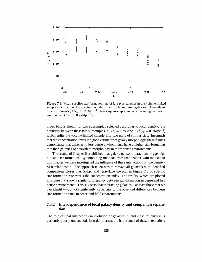
00

1 · 10−111 · 10−11

2 · 10−112 · 10−11

3 · 10−113 · 10−11

4 · 10−114 · 10−11

5 · 10−115 · 10−11

ψm

(yr−

1)

ψm

(yr−

1)

0.380.38 0.40.4 0.420.42 0.440.44 0.460.46 0.480.48 0.50.5

CC

Figure 7.6: Mean specific star formation rate of late-type galaxies in the volume limitedsample as a function of concentration index: open circles represent galaxies in lower dens-ity environments ( 1/r5 < 0.75Mpc−1), black squares represent galaxies in higher densityenvironment ( 1/r5 > 0.75Mpc−1).

index bins is shown for two subsamples selected according to local density: theboundary between these two subsamples is 1/r5 = 0.75Mpc−1 (ΣD,5 = 0.9Mpc−2)which splits the volume-limited sample into two parts of similar size. Insomuchthat the concentration index is a good estimator of galaxy morphology, these figuresdemonstrate that galaxies in less dense environments have a higher star-formationrate than galaxies of equivalent morphology in more dense environments.

The results of Chapter 6 established that galaxy-galaxy interactions trigger sig-nificant star formation. By combining methods from that chapter with the data inthis chapter we have investigated the influence of these interactions on the density-SFR relationship. The approach taken was to remove all galaxies with identifiedcompanions closer than 50 kpc and reproduce the plot in Figure 7.6 of specificstar-formation rate versus the concentration index. The results, which are plottedin Figure 7.7, show a similar discrepancy between star-formation in dense and lessdense environments. This suggests that interacting galaxies—at least those that wecan identify—do not significantly contribute to the observed differences betweenstar-formation rates in dense and field environments.

7.3.2 Interdependence of local galaxy density and companion separa-tion

The role of tidal interactions in evolution of galaxies in, and close to, clusters iscurrently poorly understood. In order to asses the importance of these interactions

128

00

1 · 10−111 · 10−11

2 · 10−112 · 10−11

3 · 10−113 · 10−11

4 · 10−114 · 10−11

5 · 10−115 · 10−11

ψm

(yr−

1)

ψm

(yr−

1)

0.380.38 0.40.4 0.420.42 0.440.44 0.460.46 0.480.48 0.50.5

CC

Figure 7.7: As Figure 7.6, but excluding all galaxies with companions closer than 50 kpc.

for the observed correlations of SSFR and morphology with density, I have in-vestigated the mean separation between galaxies and their nearest companions asa function of density. The results—presented in Figure 7.8—show, as expected, amarked decline of the mean separation at very high densities. This decline, how-ever, only becomes significant at densities around 1/r5 ≈ 1.5Mpc−1; in the range0< 1/r5 < 1.5Mpc−1 there is very little variation in the mean separation.

This is in contrast to the relations between density and morphology, and to asomewhat smaller extent SSFR, that are shown in Figures 7.4 and 7.5: they dis-play a correlation over the full range of densities that are sampled. This contrastssuggests that processing by tidal interactions between galaxies, at least ones thatthe algorithm of Section 6.1 can identify, is not the mechanism responsible for theobserved correlation of galaxy properties with density.

Light profiles

It was shown in Section 6.2 that there exists a tight relationship between the meanr-band concentration index of galaxies and projected separation to the nearest com-panion. This relationship can be summarised as follows: the concentration indexpeaks at pair separations of about 75 kpc; it rapidly declines for smaller separationsbut there is also a smaller decline for separations greater than 75 kpc.

The mean density as a function of companion separation is shown in Figure 7.9.It can be seen that there is only a weak trend of density with companion separa-tion with majority of the change occurring at a break at rp ≈ 125kpc. The es-sentially constant value of density in the range 0 < rp < 100kpc suggests that itplays little role in the decline of concentration index at close companion separ-

129

0.040.04

0.060.06

0.080.08

0.10.1

0.120.12

0.140.14

r p(M

pc)

r p(M

pc)

0.50.5 11 22 55 1010

1/r5 (Mpc−1)1/r5 (Mpc−1)

Figure 7.8: The mean projected separation to the nearest companion as a function ofdensity of environment.

ations. The density-morphology relationship can play no part in the decline inconcentration index at separations larger than 75 kpc either since Figure 7.9 showsthat mean density slightly decreases at larger separation. According to the density-morphology relationship, this should lead to an increase in the concentration indexrather than the observed decrease.

7.3.3 Tidal triggering of star formation as a function of environment

Whatever mechanisms produce the tight density-star formation relationship, theymay also affect the mechanism which triggers star formation in interacting galax-ies. This possibility is investigated by splitting the volume limited as before intotwo subsamples according to density with the boundary at 1/r5 = 0.75Mpc−1.Specific star-formation rates of these two subsamples, as functions of separation tonearest companions, are compared in Figures 7.10, 7.11 and 7.12 for late-, mixed-and early-type galaxies respectively.

The form of the SSFR-companion separation relationship for late-type galaxies(selected, as before, by requiring C > 0.375) shows remarkable similarity in denseand less dense environments. The main difference between the environments isin the magnitude of star formation across the range of pair separation: galaxies inless dense environment have a mean specific star-formation rate about 10% highercompared to galaxies in relatively more dense environment. This is in agreementwith results of Gomez et al. (2003), who showed that galaxies in dense environ-ments have smaller star-formation rates over and above what would be expected

130

0.50.5

11

22

55

10101/r

5(M

pc−

1)

1/r

5(M

pc−

1)

00 0.050.05 0.10.1 0.150.15 0.20.2 0.250.25 0.30.3

rp (Mpc)rp (Mpc)

Figure 7.9: Mean density of environment as a function of projected separation to thenearest companion for the full volume-limited sample.

00

1 · 10−101 · 10−10

2 · 10−102 · 10−10

3 · 10−103 · 10−10

4 · 10−104 · 10−10

ψm

(yr−

1)

ψm

(yr−

1)

00 0.050.05 0.10.1 0.150.15 0.20.2 0.250.25 0.30.3

Pair Separation (Mpc)Pair Separation (Mpc)

Figure 7.10: Mean specific star-formation rate as a function of separation for late-typegalaxies in the volume-limited sample split into two subsamples according to density:open circles represent galaxies in lower density environments ( 1/r5 < 0.75Mpc−1), blacksquares represent galaxies in higher density environment ( 1/r5 > 0.75Mpc−1).

131

00

5 · 10−115 · 10−11

1 · 10−101 · 10−10

1.5 · 10−101.5 · 10−10

2 · 10−102 · 10−10

ψm

(yr−

1)

ψm

(yr−

1)

00 0.050.05 0.10.1 0.150.15 0.20.2 0.250.25 0.30.3

Pair Separation (Mpc)Pair Separation (Mpc)

Figure 7.11: As Figure 7.10, but for the mixed-type galaxies.

from the density-morphology relationship only. But, it appears that density of en-vironment does not change the relative magnitude of the triggered star formationnor is the slope at separations greater than 100 kpc affected.

The effect of environment on the SSFR-companion separation relationship forgalaxies classified as mixed- and early-types is, however, very significant (Fig-ures 7.11 and 7.12). It can be seen that for these morphological types only galaxiesin the less dense environment show signature of triggered star formation, whichhas a quite high relative magnitude. The galaxies in the denser environment showlittle or no evidence of triggered star formation and even possible evidence that thestar formation rate decreases at smaller separations.

To interpret these results it is necessary to consider, besides the effects of envir-onment, the effect of misclassification of disk systems as early types due to nuclearstarbursts. One possibility is that all of the rise of specific star-formation of early-type galaxies with close companions (without taking environment into consider-ation, Figure 6.5) is due to misclassified late-type systems. Figure 7.12 can thensimply be interpreted as due that disk based systems are relatively more likely tooccur in less dense environments—this is illustrated in Figure 7.13—and thereforecan only significantly change that SSFR-rp curve.

132

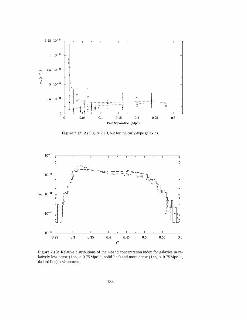
00

2.5 · 10−112.5 · 10−11

5 · 10−115 · 10−11

7.5 · 10−117.5 · 10−11

1 · 10−101 · 10−10

1.25 · 10−101.25 · 10−10ψm

(yr−

1)

ψm

(yr−

1)

00 0.050.05 0.10.1 0.150.15 0.20.2 0.250.25 0.30.3

Pair Separation (Mpc)Pair Separation (Mpc)

Figure 7.12: As Figure 7.10, but for the early-type galaxies.

10−510−5

10−410−4

10−310−3

10−210−2

10−110−1

ff

0.250.25 0.30.3 0.350.35 0.40.4 0.450.45 0.50.5 0.550.55 0.60.6

CC

Figure 7.13: Relative distributions of the r-band concentration index for galaxies in re-latively less dense (1/r5 < 0.75Mpc−1, solid line) and more dense (1/r5 > 0.75Mpc−1,dashed line) environments.

133

7.4 Tidal triggering of active galactic nuclei

7.4.1 Introduction

Active galactic nuclei are powered by energy released when matter accretes ontoblack holes (Rees, 1984). The range of luminosities of active galactic nuclei thatis observed is very large and the output from AGN appears to be episodic withdurations of strong activity less than 3× 107 yr (Heckman et al., 2004). It is anatural question to ask what triggers the active periods.

Since it now appears that many galaxies have massive black holes at theircentres (Kormendy & Richstone, 1995) it is likely that this necessary ingredientis often present. An approximate estimate of the black hole content in our volume-limited sample can be derived as follows. Mass of the black holes is stronglycorrelated with bulge velocity dispersion (Tremaine et al., 2002), with a relation ofthe form:

log (MBH/M�) = α + β log (σ/σ0) (7.1)

where σ0 = 200km s−1, α ≈ 8.1 and β ≈ 4.0. Bulge dispersions can easily beestimated for only the early-type galaxies in the volume limited sample. The meanof the dispersion for these galaxies (after exclusion of galaxies with extreme linefits) is σ ≈ 225kms−1 which implies that on average these galaxies have blackholes more massive than 108 M�.

The other necessary ingredient for an AGN is matter close enough to the blackhole to be accreted (e.g., review by Combes, 2001). Simulations, by for exampleHernquist & Mihos (1995), show that tidal interactions can very efficiently drivegas towards nuclear regions. Therefore, it has often been suggested that tidal in-teractions play an important role in fuelling AGN and that indeed there exists acausal link between galaxy interactions/mergers and AGN. The evidence for thislink, however, is not yet convincing.

A number of studies have found that galaxies exhibiting various manifesta-tions of the AGN phenomenon have an excess of close companions: Heckmanet al. (1984) find this is the case for low-redshift quasars; Heckman et al. (1985)for radio galaxies and Dultzin-Hacyan et al. (1999) for Seyfert 2 galaxies. Thereare also conflicting studies which find no significant excess companions: for ex-ample, the more recent analysis of companions of Seyferts by Schmitt (2001).Less direct evidence for tidal-triggering of AGN was presented by Sanders et al.(1988) who suggested that the ULIRGs—themselves almost universally classifiedas mergers—evolve into quasars on relatively short time scales. This too has, how-ever, been challenged by numerous authors including Tacconi et al. (2002) andDunlop et al. (2003).

7.4.2 This study

The data from the SDSS and techniques described in Chapters 5 and 6 can beused to find clear evidence of enhanced star-formation in galaxies with close com-

134

panions, presumably due to tidal triggering. I have therefore sought to use thesesame data to investigated the triggering of AGN by galaxy-galaxy interactions. Theprimary quantity that we concentrate on is [O III] luminosity which, as it originatesin the NLR far from the obscuring torus is a good and isotropic tracer of AGNluminosity (Heckman et al., 2004). Previous work often considered the fraction ofgalaxies that are AGN-dominated as a function of pair separation, but this is un-satisfactory as it requires introducing an arbitrary boundary in [O III] luminosity,which necessarily excludes lower luminosity AGN. Instead I focus on the relation-ship between [O III] luminosity and pair separation.

7.4.3 Starburst contribution to the [O III] line

As discussed in Chapter 6, there is good evidence that galaxy-galaxy interactionstrigger star formation. It was shown that two of the ways this star formation re-veals itself is the Hα emission line and the far-infrared continuum. Inevitably, thetriggered star formation will also have an effect on most of the other emission linesincluding the high-ionisation [O III] line that we propose to use to trace the outputof AGN. Disentangling the relative contributions of star formation and AGN to theobserved [O III] luminosities is essential if this line is to be used to investigate tidaltriggering of AGN.

It can be established that contamination of the [O III] line can pose a problemby considering galaxies classified as star forming (using, as before, the criteria ofSection 2.5) and late-type (using the concentration index). The [O III] luminositiesof these galaxies were calculated, as for the Hα line before, from the best-fittingGaussian curves supplied by the SDSS pipelines. Again, as before, negative valueshave been retained even though they obviously do not represent physical luminos-ities.

In Figure 7.14, the mean [O III] luminosity of these star forming galaxies as afunction of companion separation is shown. It can be seen that there is a strikingincrease in [O III] luminosity for companion separations smaller than about 75 kpc.This correlation is quite similar to that seen between the specific star formation rate(derived from Hα data) and companion separation, although the relative magnitudeof the increase is greater in the case of [O III]. One of the reasons for this may bethat although I correct for underlying stellar absorption in the case of the Hα line,no correction of any sort is made for the [O III] line. Further, the SDSS pipelinesusually report negative [O III] equivalent widths in galaxies with no emission lines,as is illustrated in the histogram of [O III] equivalent widths for ealy-, mixed- andlate-type galaxies in Figure 7.15. Therefore, it is possible that the whole distribu-tion of [O III] luminosities is shifted to smaller values, making the increase appearrelatively larger.

135

1 · 10321 · 1032

2 · 10322 · 1032

3 · 10323 · 1032

4 · 10324 · 1032

5 · 10325 · 1032

6 · 10326 · 1032

L([

Oii

i])(W

)L

([O

iii]

)(W

)

00 0.050.05 0.10.1 0.150.15 0.20.2 0.250.25 0.30.3

rp (Mpc)rp (Mpc)

Figure 7.14: Mean [O III] luminosity as a function of projected separation for late-typegalaxies in the volume limited sample.

10−510−5

10−410−4

10−310−3

10−210−2

10−110−1

100100

ff

−10−10 00 1010 2020 3030 4040 5050 6060

EW (OIII) (A)EW (OIII) (A)

Figure 7.15: Distribution of [O III] equivalent widths as reported by the SDSS pipeline forlate- (full line), mixed- (dashed line) and early-type (dotted line) galaxies that have beenclassified as not dominated by AGN. The means of the distributions are 1.35A, 0.14 A and−0.51 A respectively.

136

Figure 7.16: Distribution of galaxies in the DR2-based volume limited sample on the[O III]/Hβ vs [N II]/Hα plane. The full line shows the demarcation curve of Kauffmannet al. (2003), which is defined in Equation 7.2.

7.4.4 Measuring AGN output using the [O III] line

I use a twin approach to deal with the starburst contribution to the [O III] luminos-ity of galaxies. The first is to attempt to correct the observed [O III] luminosity forthis contribution, using the theoretical extreme line ratios for a starburst as a guide.The second is to separate galaxies into subsamples according to their separation toa BPT AGN/starburst demarcation line and compare their [O III] luminosities as afunction of companion separation. Another possible approach is to only considergalaxies completely dominated by AGN, which would make analysis simpler ascorrection for star formation would not be significant, but would produce mislead-ing results, since it has already found that galaxies with close companions haveenhanced star formation. Therefore, it is quite possible that any triggered AGNwill be accompanied by significant star formation.

In the present section, as in Section 2.5, I use the same [O III]/Hβ vs [N II]/Hαplane (Baldwin et al., 1981) for classification of galaxies. The demarcation curveused is, however, different: here I use the demarcation curve proposed by Kauff-mann et al. (2003), defined by the equation:

log

([O III]

Hβ

)>

0.61

log(

[N II]Hβ

)−0.05

+ 1.3. (7.2)

This curve was calculated so that galaxies above it include both galaxies with emis-sion line spectra dominated by AGN (classical AGN) and those with a significantbut not necessarily dominant AGN component present (‘transitional’ objects). The

137

100100

101101

102102

103103

104104

NN

00 1 · 10341 · 1034 2 · 10342 · 1034 3 · 10343 · 1034 4 · 10344 · 1034 5 · 10345 · 1034 6 · 10346 · 1034 7 · 10347 · 1034

L([O iii])(W )L([O iii])(W )

Figure 7.17: Full line: histogram of [O III] luminosities of galaxies identified as AGN ortransitional objects using the demarcation curve of Equation (7.2). Dashed line: histogramof [O III] luminosities corrected for contribution from star formation.

distribution of galaxies on the BPT plane and the demarcation curve are shown inFigure 7.16.

Correcting [O III] luminosities for stellar contribution

The observed [O III] luminosities of galaxies classified as AGN were separated intoa contribution from the AGN and star formation by finding the minimum [O III]flux needed to move the galaxy from the demarcation curve (Eq. 7.2) to its observedposition on the BPT diagram. The exact procedure was as follows.

Let the observed position of a galaxy on the BPT diagram be designated by(x,y) where x = log([N II]/Hα) and y = log([O III]/Hβ ). If the locus of points onthe demarcation curve is represented by (xd,yd), then the distance in the log-logplane from the observed point to the curve is just δ =

√(x− xd)2 + (y− yd)2. I

denote the minimum distance δ as ∆ and the corresponding point on the curve(x0,y0). As the curve defined by Equation 7.2 describes the most extreme lineratios that can be attributed to a pure starburst, the ratio corresponding to (x0,y0)describes the closest pure starburst to the observed galaxy line ratios.

Using the very conservative assumption that all of the measured Hβ flux isassociated with star formation, the [O III] luminosity associated with star form-ation is simply Hβ × 10y0 . The distribution of corrected and uncorrected [O III]luminosities is shown in Figure 7.17.

138

00

0.0250.025

0.050.05

0.0750.075

0.10.1

0.1250.125

ff

00 0.50.5 11 1.51.5 22

∆∆

Figure 7.18: Full line: histogram of the separation on the log [O III]/Hα vs. log [N II]/Hβplane from the demarcation line of Equation (7.2) to the observed line ratios for all galaxiesclassified as AGN or transitional. Dashed line: histogram of the same distance but for thestar-forming objects.

Quantifying relative importance of star-formation and AGN

The alternative approach is to simply quantify the relative importance of the AGNand star formation and investigate how the observed correlation changes with thisparameters. This can be conveniently done using the distance ∆ from starburst/AGNdemarcation line. This distribution of this distance is shown in Figure 7.18.

7.4.5 Results

I proceed in a similar fashion to the earlier study of triggering of star formation andplot, in Figure 7.19, the mean [O III] luminosity against projected separation to thenearest companion, for all of the galaxies identified as AGN or transitional objectsusing the boundary defined by Equation 7.2.

The open circles in Figure 7.19 show the uncorrected [O III] luminosity: itcan be seen that there is some evidence for an enhancement at separations belowapproximately 75 kpc. The corrected [O III] luminosity (filled squares), however,shows no evidence for enhancement at all, and possibly some for a small decreaseof the mean [O III] luminosity at close separation. It is possible that it is decreaseis due to an over-correction for the contribution from star formation.

As an alternative, I do not use the corrected [O III] luminosities but insteadconsider the un-corrected [O III] luminosity versus companion separation for sub-samples defined according to distance from the demarcation line. In Figure 7.20,

139

5 · 10325 · 1032

1 · 10331 · 1033

1.5 · 10331.5 · 1033

2 · 10332 · 1033

2.5 · 10332.5 · 1033

3 · 10333 · 1033

L([

Oii

i])(W

)L

([O

iii]

)(W

)

00 0.050.05 0.10.1 0.150.15 0.20.2 0.250.25 0.30.3

rp (Mpc)rp (Mpc)

Figure 7.19: Open circles: mean [O III] luminosity as a function of separation to nearestcompanion for galaxies in the volume-limited sample classified as containing significantAGN. Filled squares: as open circles but [O III] luminosities have been corrected for con-tribution by star formation.

I plot this L([O III]) vs rp relationship for the galaxies close to the demarcationcurve, namely star-forming galaxies with a distance 0 < ∆ < 0.1 and AGN galax-ies with a distance 0 < ∆ < 0.25 from the curve. It can be seen that although theAGN galaxies have higher mean [O III] luminosities, these two sets follow a sim-ilar trend with respect to companion separation. In Figure 7.21, the same two setsof galaxies are shown, but also shown are the more extreme AGN galaxies, thatis those with a distance 0.25 < ∆ < 1 from the demarcation curve. It can be seenthat these strongly AGN dominated galaxies show, in contrast to the star-forminggalaxies, little if any enhancement of [O III] luminosity at close separations.

It can therefore be concluded that, although both star formation dominatedsystems and systems dominated by AGN show an increase of [O III] luminosityat closer pair separations, this can be adequately explained in both of the classesby enhanced star formation alone. These results suggest that if galaxy interactionsare a trigger of AGN, this triggering must occur at a significantly later stage ofinteraction then star formation. These later stages are not adequately traced by thecompanion finding algorithm that I employ.

140

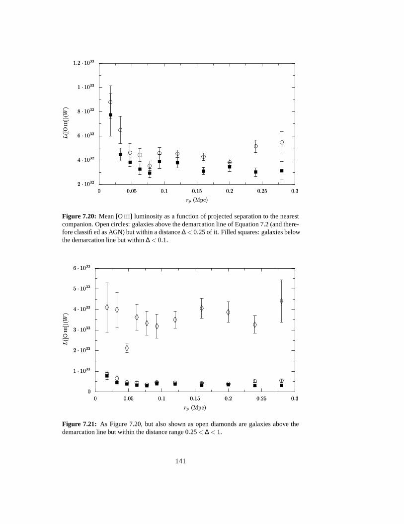
2 · 10322 · 1032

4 · 10324 · 1032

6 · 10326 · 1032

8 · 10328 · 1032

1 · 10331 · 1033

1.2 · 10331.2 · 1033L

([O

iii]

)(W

)L

([O

iii]

)(W

)

00 0.050.05 0.10.1 0.150.15 0.20.2 0.250.25 0.30.3

rp (Mpc)rp (Mpc)

Figure 7.20: Mean [O III] luminosity as a function of projected separation to the nearestcompanion. Open circles: galaxies above the demarcation line of Equation 7.2 (and there-fore classified as AGN) but within a distance ∆< 0.25 of it. Filled squares: galaxies belowthe demarcation line but within ∆ < 0.1.

00

1 · 10331 · 1033

2 · 10332 · 1033

3 · 10333 · 1033

4 · 10334 · 1033

5 · 10335 · 1033

6 · 10336 · 1033

L([

Oii

i])(W

)L

([O

iii]

)(W

)

00 0.050.05 0.10.1 0.150.15 0.20.2 0.250.25 0.30.3

rp (Mpc)rp (Mpc)

Figure 7.21: As Figure 7.20, but also shown as open diamonds are galaxies above thedemarcation line but within the distance range 0.25< ∆ < 1.

141

142

Chapter 8

Conclusions

A two pronged approach has been taken to study star formation in galaxies: a stat-istical study designed to representatively sample the range of star-formation ratesfound in the local universe; and, development and application of some techniquesuseful for understanding the more intensely star-forming systems.

The statistical study has been carried out, as far possible, with the aim of min-imising and quantifying biases. To a large measure, this has been made possibleby the SDSS which, by combining an imaging survey, r-band selection, wide spec-tral range and sophisticated spectral fitting, is providing survey data of unpreced-ented quality. I have built upon this intrinsic completeness by using a volume(0.03 < z < 0.1) and luminosity (Mr <−20.45) limited sample, by making use ofthe imaging data for pair selection and by using a well defined criterion for min-imum pair separation. I have also begun to jointly consider a number of factorswhich control the observed star-formation rates of galaxies. These include mor-phology, galaxy-galaxy interactions and environment. The conclusions may besummarised as follows:

(i) It has been shown that there exists an anti-correlation between specific star-formation rates of galaxies and projected separation to their nearest compan-ions. This is interpreted to be due to tidal triggering of star formation whichbecomes apparent at projected companion separations below approximately50 kpc.

(ii) The robustness of this result, which was derived from aperture and extinc-tion corrected Hα data, has been demonstrated by making use of IRAS far-infrared observations. It is found that, for the subsample of galaxies detectedby IRAS, far-infrared and Hα derived star-formation rates agree closely inboth magnitude and trend with projected separation to the nearest compan-ion.

(iii) The concentration index, that is the ratio of half- and 90 percent-light radii,has been used as a proxy for morphological classification of galaxies in thevolume limited sample and their companions. It is found that morphology

143

is a dominant controlling factor of star-formation rates compared to tidalinteractions.

(iv) I find no evidence that the morphological type of the companion nor its mass(within the factor of approximately 6 that is probed) influences the mag-nitude of triggered star formation.

(v) There is a marked correlation between the concentration index and pair sep-arations in the range 15kpc < rp < 75kpc, i.e., galaxies with close com-panion have significantly more concentrated light profiles. This has beeninterpreted as evidence that tidal interactions preferentially trigger nuclearstar formation.

(vi) The luminosity of the [O III] line, which is a widely used proxy for the totalAGN luminosity, is strongly anti-correlated with separation to the nearestcompanion, even more so than the star-formation rate. This anti-correlationis, however, found to be consistent, in both star formation-dominated andAGN-dominated galaxies, with triggered star formation only. Therefore, noevidence for tidal triggering of AGN is found for the range of companionseparations (rp ' 15kpc) that have been probed.

(vii) A remarkable independence, at the present time at least, is found betweentidal interactions and the density/star-formation rate correlation: firstly, itwas shown that interacting systems do not contribute to the observed rela-tionship between the density and the star-formation rate; secondly, the mag-nitude and onset of tidal triggering of star formation appears to be independ-ent of density of environment, although the overall star-formation rates arelower in the more dense environments.

As a step toward understanding intensely star forming and highly obscuredgalaxies, some modelling techniques of emission from nuclear starbursts have beendeveloped. A key part of this is a comprehensive, physically based, dust modelfrom which both absorption and emission of radiation by dust are calculated. Arange of dust particle radii for three species of grains is taken into account in themodel as well as an accurate treatment of single-photon heating and subsequentemission. Such a dust model allows quantitative predictions of how changes in thedust grain population will affect galaxy spectra. In conjunction with this, a newphysically motivated way of representing breakdown of dust particles is proposed.

New, sub-arcsecond resolution, mid-infrared imaging of a sample of nearbystar formating and/or AGN-powered galaxies has also been presented. These datahave been used in combination with published observations to produce detailedmodels of two systems: the moderate nuclear starburst NGC 520 and the ULIRGArp 220.

The conclusions drawn may be summarised as follows:

144

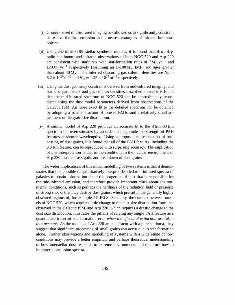
(i) Ground-based mid-infrared imaging has allowed us to significantly constrainor resolve the dust emission in the nearest examples of infrared-luminousobjects.

(ii) Using STARBURST99 stellar synthesis models, it is found that Brα , Brγ ,radio continuum and infrared observations of both NGC 520 and Arp 220are consistent with starbursts with star-formation rates of 7M� yr−1 and120M� yr−1 respectively (assuming an 1–100 M� IMF) and ages greaterthan about 40 Myr. The inferred obscuring gas column densities are NH =6.2×1026 m−2 and NH = 1.25×1027 m−2 respectively.

(iii) Using the dust geometry constraints derived from mid-infrared imaging, andstarburst parameters and gas column densities described above, it is foundthat the mid-infrared spectrum of NGC 520 can be approximately repro-duced using the dust model parameters derived from observations of theGalactic ISM. An more exact fit to the detailed spectrum can be obtainedby adopting a smaller fraction of ionised PAHs, and a relatively small ad-justment of the grain size distribution.

(iv) A similar model of Arp 220 provides an accurate fit to the 8 µm–30 µmspectrum but overestimates by an order of magnitude the strength of PAHfeatures at shorter wavelengths. Using a proposed representation of pro-cessing of dust grains, it is found that all of the PAH features, including the3.3 µm feature, can be reproduced with surprising accuracy. The implicationof this interpretation is that in the conditions in the nuclear environment ofArp 220 must cause significant breakdown of dust grains.

The wider implications of this initial modelling of two systems is that it demon-strates that it is possible to quantitatively interpret detailed mid-infrared spectra ofgalaxies to obtain information about the properties of dust that is responsible forthe mid-infrared emission, and therefore provide important clues about environ-mental conditions, such as perhaps the hardness of the radiation field or presenceof strong shocks that may destroy dust grains, which prevail in the generally highlyobscured regions of, for example, ULIRGs. Secondly, the contrast between mod-els of NGC 520, which requires little change to the dust size distribution from thatobserved in the Galactic ISM, and Arp 220, which requires a drastic change to thedust size distribution, illustrates the pitfalls of relying any single PAH feature as aquantitative tracer of star formation even when the effects of extinction are takeninto account. As the models of Arp 220 are consistent with a pure starburst, theysuggest that significant processing of small grains can occur due to star formationalone. Further observations and modelling of systems with a wide range of ISMconditions may provide a better empirical and perhaps theoretical understandingof how interstellar dust responds to extreme environments and therefore how tointerpret its emission spectra.

145

146

Appendix A

Implementation details

A.1 Dust model

A.1.1 PAH absorption cross sections

The code to calculate the PAH absorption cross sections was implemented as fol-lows.

Listing A.1: Definition of the Drude profiles for neutral and ionised PAH molecules; thecolumns show the wavelength (in µm), γ which is the parameter that controls the width ofthe feature and σ which is the intensity of the feature in the units of 10−20 cmC−1.

double b n d u s t p a h d a t a d r u d e p r o f s n e u t r a l [ 1 4 ] [ 3 ] = {{ . 0 7 2 2 , 0 . 1 9 5 , 7 . 9 7 e7 } ,{ . 2 1 7 5 , 0 . 2 1 7 , 1 . 2 3 e7 } ,{ 3 . 3 , 0 . 0 1 2 , 1 9 7 } ,

5 { 6 . 2 , 0 . 0 3 2 , 1 9 . 6 } ,{7 . 7 , 0 . 0 9 1 , 6 0 . 9 } ,{ 8 . 6 , 0 . 0 4 7 , 3 4 . 7 } ,{11 .3 , 0 . 0 1 8 , 4 2 7 } ,{11 .9 , 0 . 0 2 5 , 7 2 . 7 } ,

10 {12 .7 , 0 . 0 2 4 , 1 6 7 } ,{ 1 6 . 4 , 0 . 0 1 0 , 5 . 5 2 } ,{ 1 8 . 3 , 0 . 0 3 6 , 6 . 0 4 } ,{21 .2 , 0 . 0 3 8 , 1 0 . 8 } ,{ 2 3 . 1 , 0 . 0 4 6 , 2 . 7 8} ,

15 { 2 6 . 0 , 0 . 6 9 , 1 5 . 2 } } ;

double b n d u s t p a h d a t a d r u d e p r o f s i o n i s e d [ 1 4 ] [ 3 ] = {{ . 0 7 2 2 , 0 . 1 9 5 , 7 . 9 7 e7 } ,{ . 2 1 7 5 , 0 . 2 1 7 , 1 . 2 3 e7 } ,

20 { 3 . 3 , 0 . 0 1 2 , 4 4 . 7 } ,{ 6 . 2 , 0 . 0 3 2 , 1 5 7 } ,{7 . 7 , 0 . 0 9 1 , 5 4 8 } ,{ 8 . 6 , 0 . 0 4 7 , 2 4 2 } ,{11 .3 , 0 . 0 1 8 , 4 0 0 } ,

147

25 {11 .9 , 0 . 0 2 5 , 6 1 . 4 } ,{12 .7 , 0 . 0 2 4 , 1 4 9 } ,{ 1 6 . 4 , 0 . 0 1 0 , 5 . 5 2 } ,{ 1 8 . 3 , 0 . 0 3 6 , 6 . 0 4 } ,{21 .2 , 0 . 0 3 8 , 1 0 . 8 } ,

30 { 2 3 . 1 , 0 . 0 4 6 , 2 . 7 8 } ,{ 2 6 . 0 , 0 . 6 9 , 1 5 . 2 } } ;

Listing A.2: Code that implements Drude profiles

double b n d u s t d r u d e ( double x , double x0 , double gamma ){

re turn 2 . 0 / M PI ∗ ( x0 ∗ gamma ) /( pow ( x / x0 −x0 / x , 2 ) + pow ( gamma , 2 ) ) ;

5 }

Listing A.3: Code that calculates the PAH cross sections.

double bndust CAbsPAH ( double a ,double lambda ,double pahbands [ 1 4 ] [ 3 ] ,b n d u s t p a h e n h a n c e m e n t s ∗ e )

5 {

/ / number o f carbon atomsdouble Nc = bndust PAHaToNc ( a ) ;

10 /∗ lambda m u s t be i n micron f o r t h i s t o work ∗ /double x = 1 . 0 / lambda ;

/ / Number o f hydrogen atomsdouble hc = bndust PAHNctoHc ( Nc ) ;

15

i f ( x > 1 7 . 2 5 ){

re turn bndus t CAbsGraph ( a , lambda ) ;}

20 e l s e i f ( x> 15 &&x <= 1 7 . 2 5 )

{re turn ( 1 2 6 . 0 − 6 . 4 9 4 3 ∗ x ) ∗

1e−18 ∗ Nc ;25 }

e l s e i f ( x> 10 &&x <= 1 5 )

{re turn

30 ( bndus t PahDrudeCS ( pahbands ,0 , hc ,e ,lambda ) +

148

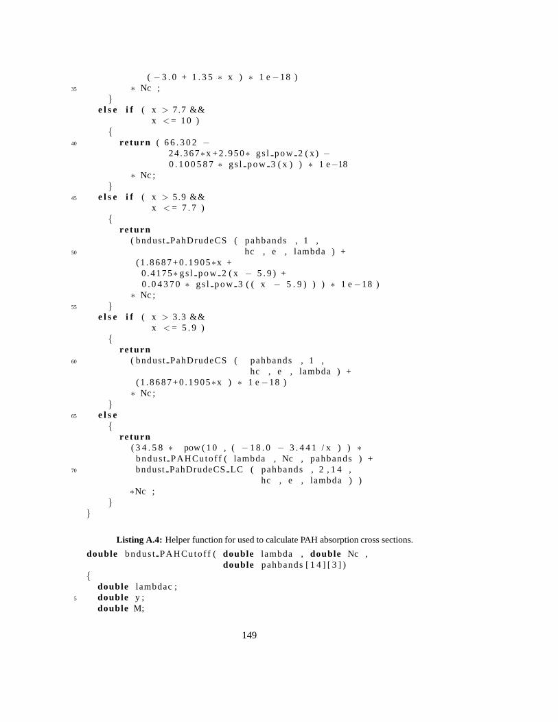
( − 3 . 0 + 1 . 3 5 ∗ x ) ∗ 1 e−18 )35 ∗ Nc ;

}e l s e i f ( x > 7.7 &&

x <= 1 0 ){

40 re turn ( 6 6 . 3 0 2 −24 .367∗x + 2 . 9 5 0∗ g s l p o w 2 ( x ) −0 . 1 0 0 5 8 7 ∗ g s l p o w 3 ( x ) ) ∗ 1 e−18

∗ Nc ;}

45 e l s e i f ( x > 5.9 &&x <= 7 . 7 )

{re turn

( bndus t PahDrudeCS ( pahbands , 1 ,50 hc , e , lambda ) +

( 1 . 8 6 8 7 + 0 . 1 9 05∗x +0 .4175∗ g s l p o w 2 ( x − 5 . 9 ) +0 . 0 4 3 7 0 ∗ g s l p o w 3 ( ( x − 5 . 9 ) ) ) ∗ 1 e−18 )

∗ Nc ;55 }

e l s e i f ( x > 3.3 &&x <= 5 . 9 )

{re turn

60 ( bndus t PahDrudeCS ( pahbands , 1 ,hc , e , lambda ) +

( 1 . 8 6 8 7 + 0 . 1 9 05∗x ) ∗ 1 e−18 )∗ Nc ;

}65 e l s e

{re turn

( 3 4 . 5 8 ∗ pow ( 1 0 , ( − 1 8 . 0 − 3 . 4 4 1 / x ) ) ∗bndus t PAHCutof f ( lambda , Nc , pahbands ) +

70 bndust PahDrudeCS LC ( pahbands , 2 , 1 4 ,hc , e , lambda ) )

∗Nc ;}

}

Listing A.4: Helper function for used to calculate PAH absorption cross sections.

double bndus t PAHCutof f ( double lambda , double Nc ,double pahbands [ 1 4 ] [ 3 ] )

{double lambdac ;

5 double y ;double M;

149

i f ( Nc > 4 0 ) M = 0 . 4 ∗ Nc ;e l s e M= 0 . 3 ∗ Nc ;

10

i f ( b n d u s t P A H I o n i s a t i o n ( pahbands ) ) {lambdac = 1 . 0 / ( 2 . 2 8 2 ∗ pow (M, − 0 . 5 ) + 0 . 8 8 9 ) ;

} e l s e {lambdac = 1 . 0 / ( 3 . 8 0 4 ∗ pow (M, − 0 . 5 ) + 1 . 0 5 2 ) ;

15 }y = lambdac / lambda ;

re turn 1 . 0 / M PI ∗a t a n 2 ( ( 1 e3 ∗ pow ( ( y − 1 ) , 3 ) ) , y ) + 0 . 5 ;

20 } ;

double bndus t PahDrudeCS ( double d a t a [ 1 4 ] [ 3 ] ,unsigned j , double hc ,b n d u s t p a h e n h a n c e m e n t s ∗ e ,

25 double lambda ){

double lambda0 ;double gamma ;double sigma ;

30

b n d u s t G e t P a h D r u d e P r o f ( da ta , j , hc , e , & lambda0 ,& gamma , & sigma ) ;

/ / Lambda i s i n micron b u t35 / / c r o s s s e c t i o n i n cm ˆ 2 ( sigma i s i n cm ˆ 1 )

/ / −− t h u s need t o m u l t i p l y by 1 e−4re turn b n d u s t d r u d e ( lambda , lambda0 , gamma)∗ 1 e−4 ∗ sigma ;

40 }

double bndust PahDrudeCS LC ( double d a t a [ 1 4 ] [ 3 ] ,unsigned jmin ,unsigned jmax ,

45 double hc ,b n d u s t p a h e n h a n c e m e n t s ∗ e ,double lambda ) {

double r e s = 0 ;unsigned j ;

50 f o r ( j = jmin ; j < jmax ; j + + )r e s + = bndus t PahDrudeCS ( da ta , j , hc , e , lambda ) ;

re turn r e s ;}

150

10−2610−26

10−2510−25

10−2410−24

10−2310−23

10−2210−22

10−2110−21C

abs(m

2)

Cabs(m

2)

1 · 10−61 · 10−6 2 · 10−62 · 10−6 5 · 10−65 · 10−6 1 · 10−51 · 10−5 2 · 10−52 · 10−5 5 · 10−55 · 10−5 1 · 10−41 · 10−4

a (m)a (m)

Figure A.1: Absorption cross section of an ionised (full line) and neutral (dashed line)PAH with 40 carbon atoms.

10−2510−25

10−2410−24

10−2310−23

10−2210−22

10−2110−21

10−2010−20

10−1910−19

10−1810−18

Cabs(m

2)

Cabs(m

2)

10−910−9 10−810−8 10−710−7 10−610−6

a (m)a (m)

Figure A.2: As Figure A.1, but showing the optical, UV, and far-UV absorption crosssection.

151

11

22

55

1010

2020

5050

100100

200200

500500

10001000

NN

1 · 10−211 · 10−21 2 · 10−212 · 10−21 5 · 10−215 · 10−21 1 · 10−201 · 10−20 2 · 10−202 · 10−20 5 · 10−205 · 10−20

E (J)E (J)

Figure A.3: Cumulative energy distribution of model normal modes of a PAH moleculewith 40 carbon atoms. The two sets of modes with different Debye temperatures are evidentby the change of slope at E ≈ 1.2×10−20 J as well as the three sets of fixed-energy modes(the C–H modes) which are evident by the three jumps.

A.1.2 Normal mode spectra

The normal mode spectra were calculated using the approximation that they areuniformly distributed in k-space up to a cut-off energy corresponding to the Debyetemperature ΘD.

For PAHs, we separately calculated the in-plane C–C modes (ΘD = 2504K)and out-of-plane C–C modes (ΘD = 863K). The normal modes corresponding tothe C–H modes were assigned energies of observed mid-infrared features: hc/E =3.3 µm, hc/E = 8.6 µm and hc/E = 11.3 µm for the stretch, in-plane bend andout-of-plane bend modes respectively.

For the silicate grains a combination of 2-dimensional (accounting for two-thirds of the available modes) and 3-dimensional (accounting for the remainingthird of modes) Debye spectra were used with Debye temperatures of ΘD = 500Kand ΘD = 1500K respectively.

152

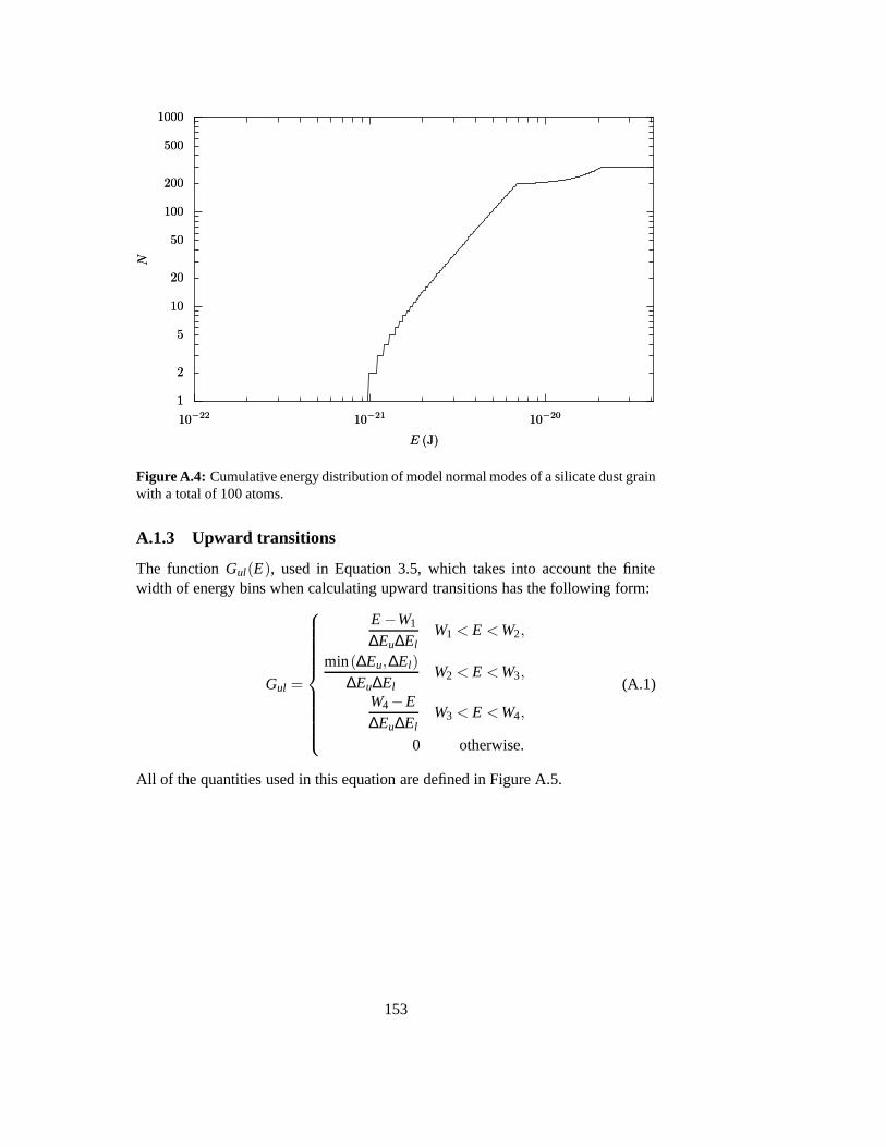
11

22

55

1010

2020

5050

100100

200200

500500

10001000

NN

10−2210−22 10−2110−21 10−2010−20

E (J)E (J)

Figure A.4: Cumulative energy distribution of model normal modes of a silicate dust grainwith a total of 100 atoms.

A.1.3 Upward transitions

The function Gul(E), used in Equation 3.5, which takes into account the finitewidth of energy bins when calculating upward transitions has the following form:

Gul =

E−W1

∆Eu∆ElW1 < E <W2,

min(∆Eu,∆El)

∆Eu∆ElW2 < E <W3,

W4−E∆Eu∆El

W3 < E <W4,

0 otherwise.

(A.1)

All of the quantities used in this equation are defined in Figure A.5.

153

Eminl

Emaxl

Eminu

Emaxu

W1 W2 W3 W4

∆El

∆Eu

Figure A.5: Illustration of the energy boundaries used in function Gul(E). Note that W2 isthe smaller and W3 the larger of the pair of values: (Emax

l −Emaxu ) and (Emin

l −Eminu ).

154

Appendix B

Phase retrieval holography usingastronomical sources

B.1 Preface

Besides the work presented in the main part of this thesis, I have been involved indevelopment of a novel technique, described in this section, to characterise surfacesof radio, millimetre and sub-millimetre telescopes. The original concept and exper-imental implementation of this technique was developed by Prof. R. E. Hills duringearly operations of the James Clerk Maxwell Telescope (JCMT) on Mauna Kea.The implementation described here was developed by Prof. Hills, Dr. J. Richerand myself over the space of last four years. We have been assisted in this develop-ment by a number of people whose contributions it is a pleasure to acknowledge:J. Wouterloot and P. Friberg at the JCMT for providing us data; C. Chandler whoresponsible for the testing of the technique at the Green Bank Telescope (GBT)and the rest of the surface team at the GBT, particularly R. Prestage, R. Maddalenaand D. Balser.

At the present time, this technique is not routinely employed at the major obser-vatories. However, the system we have developed is now reaching maturity and isexpected to be deployed for routine use at the GBT in Winter/Spring 2004/2005. Inaddition, some useful measurements of other antennas has been already obtained.Therefore, although none of the investigations in the main body of the thesis couldbe said to have benefited from this technique, similar studies, especially of atom-ic/molecular gas and dust, in the future perhaps will.

B.2 Introduction

Measuring the deformations of telescope antennas using microwaves (often calledholography) is useful both for direct corrections of surface errors, and as an in-put into theoretical models of the telescope mechanics. Both of those are in turninvaluable for the recent generation of telescopes with actuator-adjustable, and in

155

some case active, surfaces. Maximising the surface accuracy of existing and newantennas is of increasing scientific importance for two reasons: it increases thegain, so allowing detection of fainter compact sources, and it reduces the amountof power in the ‘error beam’, so allowing higher dynamic range imaging of exten-ded sources.

In the phase-retrieval approach to millimetre-wave holography, only the powerpattern of the antenna is measured, usually at two or more different focus settings.The phase of the signal in the aperture is later recovered by numerical processing.This technique has been applied with considerable success on a number of largeantennas, but usually only with artificial sources, i.e. transmitters on the ground oron spacecraft.

The technique described here is suitable for measuring surface errors with mod-erate spatial resolution by observing astronomical sources, using existing astro-nomical receivers on the telescopes. This new approach uses numerical fitting ofa parameterised description of the surface errors, and of the amplitude of the re-ceiver’s illumination pattern. The technique is flexible. It can be adapted straight-forwardly to various different observational techniques, including total power ob-servations, and the various differencing schemes which involve movement of thesecondary mirror (‘beam switching’) and/or primary mirror (‘nodding’). The in-creasing availability of astronomical array detectors makes the mapping processparticularly quick and efficient.

This section is based in part on the paper by Nikolic et al. (2002). We expectto publish a full account of the technique and results in the near future.

B.3 Description of technique

If we can measure both the amplitude and phase of the beam pattern in the far field,a simple Fourier inversion will give us the aperture function (this is with-phaseholography). However, measuring just the power pattern will under-determine theaperture function (e.g., inverting the sign of the errors produces the same powerpattern). We can break this degeneracy by measuring power patterns at a numberof focus settings, which produces partially independent data sets.

A straightforward inversion is still not possible due to non-linearity, so we haveemployed a numerical fitting algorithm. We parameterise the surface in terms of afixed number of coefficients of Zernike circle polynomial functions (see, e.g., Born& Wolf 1970 for a definition). Besides being orthonormal on the unit circle, theyalso have the advantage that by restricting the highest order used, the results arenot sensitive to the poorly-constrained, small-scale errors on the surface. The dataobtained so far have allowed us to fit a model including terms up to radial orderabout 6: the smallest spatial scale contained in the model then corresponds to ap-proximately one sixth the primary mirror diameter. Depending on signal to noiseof the data and any systematic effects (such as pointing errors), it may be possibleto probe smaller scales than this. Other free parameters in the model are the posi-

156

tion and width of the primary reflector illumination (modelled as a Gaussian), thedirections and sizes of the chopping and nodding motions, and optionally the comaerror term introduced by the chopping of the secondary.

The best fit surface is then found by minimising differences between the ob-served and simulated data, with appropriate weightings to take into account thenoise. In order to allow for possibility of beam maps which are not sampled ona regular grid—this in fact is the normal mode of operation—simulated sky mapsare interpolated to position of each of the observed data points for comparison.This eliminates the need for any re-griding of observed data which is essential topreserve information about structure of the whole dish.

The noise is modelled as a sum of additive (thermal) and proportional-to-signal components. We use a public-domain Levenberg-Marquardt minimisationalgorithm (Meyerdierks et al., 1997) with numerically calculated derivatives, whichwe have found to be efficient and reliable for this problem. As an independentcheck, analyses during the initial stages of the project also employed the downhill-simplex minimisation algorithm (Press et al., 1992). With reasonable quality data,we usually see good convergence and no local minima.

Any bright source of known shape is suitable for this method. Quasars are thenatural choice at low frequencies, but at submillimetre wavelengths, planets aremuch brighter. Because our technique uses a fitting algorithm, it is possible to takeaccount of any extension of the source (e.g., the planet’s disc) if it is accuratelyknown.

We have performed several simulations of the technique, by generating syn-thetic data and deriving estimates of the surface from them. These have allowedus to validate the robustness of the method, and allowed us to estimate the optimalsize of the defocus term to use, and the signal-to-noise required to measure a givennumber of Zernike terms. An example of signal to noise predictions derived froma set of observations is shown in Figure B.1.

B.4 Results

We have tested the technique using data obtained at the JCMT and GBT. The resultspresented here are for the GBT because their interpretation is more straightforward.In case of data taken with the SCUBA instrument at the JCMT it is not clear howaberrations in the imaging optics of the camera affect the derived phase maps.

The GBT is a 100-m off-axis paraboloid telescope, designed for frequencies upto around 100 GHz. All of the higher frequency receivers operate at a Gregorianfocus. There have so far been three testing campaigns at the GBT during which asignificant quantity of data has been collected. Both continuum and spectral linedata has been used.

Because of the off-axis geometry, the phase change in the aperture plane cor-responding to a defocus of the telescope is more complicated then that of a standardCassegrain design like the JCMT where it is a simple radial function. It is described

157

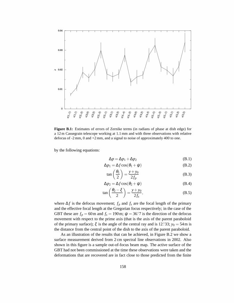
00

0.010.01

0.020.02

0.030.03

0.040.04

σσ

z(1,

-1)

z(1,

-1)

z(1,

1)z(

1,1)

z(2,

-2)

z(2,

-2)

z(2,

0)z(

2,0)

z(2,

2)z(

2,2)

z(3,

-3)

z(3,

-3)

z(3,

-1)

z(3,

-1)

z(3,

1)z(

3,1)

z(3,

3)z(

3,3)

z(4,

-4)

z(4,

-4)

z(4,

-2)

z(4,

-2)

z(4,

0)z(

4,0)

z(4,

2)z(

4,2)

z(4,

4)z(

4,4)

z(5,

-5)

z(5,

-5)

z(5,

-3)

z(5,

-3)

z(5,

-1)

z(5,

-1)

z(5,

1)z(

5,1)

z(5,

3)z(

5,3)

z(5,

5)z(

5,5)

Figure B.1: Estimates of errors of Zernike terms (in radians of phase at dish edge) fora 12 m Cassegrain telescope working at 1.1 mm and with three observations with relativedefocus of -2 mm, 0 and +2 mm, and a signal to noise of approximately 400 to one.

by the following equations:

∆p = ∆p1 + ∆p2 (B.1)

∆p1 = ∆ f cos(θ1 + ψ) (B.2)

tan

(θ1

2

)=

y + y0

2 fp(B.3)

∆p2 = ∆ f cos(θ2 + ψ) (B.4)

tan

(θ2−ξ

2

)=

y + y0

2 fs, (B.5)

where ∆ f is the defocus movement; fp and fs are the focal length of the primaryand the effective focal length at the Gregorian focus respectively; in the case of theGBT these are fp = 60m and fs = 190m; ψ = 36.◦7 is the direction of the defocusmovement with respect to the prime axis (that is the axis of the parent paraboloidof the primary surface); ξ is the angle of the central ray and is 12.◦33; y0 = 54m isthe distance from the central point of the dish to the axis of the parent paraboloid.

As an illustration of the results that can be achieved, in Figure B.2 we show asurface measurement derived from 2 cm spectral line observations in 2002. Alsoshown in this figure is a sample out-of-focus beam map. The active surface of theGBT had not been commissioned at the time these observations were taken and thedeformations that are recovered are in fact close to those predicted from the finite

158

Figure B.2: Calculated aperture function for the GBT; Left: phase, Middle: amplitude,Right: an example of an out-of-focus map

element models of the GBT structure.

B.5 Conclusions

This technique for measurement or large-scale surface errors has several benefits.Most importantly, it allows measurement of the surface at many different eleva-tion angles, so allowing the measurement of gravitationally-induced deformations,which should be mainly large scale. The technique is also low cost both in termsof money and time: it uses existing instrumentation, and the maps can usually bemade in short periods, usually less than half an hour of observing time. In ad-dition, as receivers are upgraded and made more sensitive, the technique benefitsfrom automatic increases in speed and accuracy. The technique is most likely to beuseful when used as an extra diagnostic of antenna behaviours in conjunction witha conventional transmitter-based holography system which measures accurately thesmall scale errors.

159

160

Bibliography

Abazajian K., et al., 2004, AJ, 128, 502

Abraham R. G., Valdes F., Yee H. K. C., van den Bergh S., 1994, ApJ, 432, 75

Alexander T., Lutz D., Sturm E., Genzel R., Sternberg A., Netzer H., 2000, ApJ,536, 710

Allamandola L. J., Tielens G. G. M., Barker J. R., 1989, ApJS, 71, 733

Antonucci R., 1993, ARA&A, 31, 473

Arp H., 1966, Atlas of peculiar galaxies. Pasadena: California Inst. Technology,1966

Baker J. G., Menzel D. H., 1938, ApJ, 88, 52

Baldwin J. A., Phillips M. M., Terlevich R., 1981, PASP, 93, 5

Ball N. M., Loveday J., Fukugita M., Nakamura O., Okamura S., Brinkmann J.,Brunner R. J., 2004, MNRAS, 348, 1038

Balogh M., et al., 2004, MNRAS, 348, 1355

Barnes J. E., Hernquist L., 1992, ARA&A, 30, 705

Barnes J. E., Hernquist L. E., 1991, ApJ, 370, L65

Barton E. J., Geller M. J., Kenyon S. J., 2000, ApJ, 530, 660

Becker R. H., White R. L., Helfand D. J., 1995, ApJ, 450, 559

Bell E. F., 2003, ApJ, 586, 794

Bell E. F., McIntosh D. H., Katz N., Weinberg M. D., 2003, ApJS, 149, 289

Bergvall N., Laurikainen E., Aalto S., 2003, A&A, 405, 31

Blain A. W., Barnard V. E., Chapman S. C., 2003, MNRAS, 338, 733

Blanton M. R., Eisenstein D. J., Hogg D. W., Schlegel D. J., Brinkmann J., 2003a,ArXiv Astrophysics e-print astro-ph/0310453

161

Blanton M. R., Lin H., Lupton R. H., Maley F. M., et al., 2003b, AJ, 125, 2276

Blanton M. R., et al., 2003c, AJ, 125, 2348

Blitz L., Williams J. P., 1999, in NATO ASIC Proc. 540: The Origin of Stars andPlanetary Systems, pp. 3–28

Bohren, Huffman, 1998, Absorption and Scattering of Light by Small Particles.Wiley Science Paperback Series

Boksenberg A., Carswell R. F., Allen D. A., Fosbury R. A. E., Penston M. V.,Sargent W. L. W., 1977, MNRAS, 178, 451

Born, Wolf, 1970, Principles of Optics, Pergamon

Brinchmann J., Charlot S., White S. D. M., Tremonti C., Kauffmann G., HeckmanT., Brinkmann J., 2004, MNRAS, 351, 1151

Burbidge E. M., Burbidge G. R., Hoyle F., 1963, ApJ, 138, 873

Bushouse H. A., Werner M. W., 1990, ApJ, 359, 72

Caplan J., Deharveng L., 1986, A&A, 155, 297

Cardelli J. A., Clayton G. C., Mathis J. S., 1989, ApJ, 345, 245

Carral P., Turner J. L., Ho P. T. P., 1990, ApJ, 362, 434

Charlot S., Longhetti M., 2001, MNRAS, 323, 887

Clements D. L., et al., 2002, ApJ, 581, 974

Colless M., et al., 2001, MNRAS, 328, 1039

Combes F., 2001, in Advanced Lectures on the Starburst-AGN (also,astro-ph/0010570), Aretxaga, Kunth, Mujica, eds., Singapore: World Scientific

Condon J. J., 1992, ARA&A, 30, 575

Condon J. J., et al., 2003, AJ, 125, 2411

Cox M. J., Eales S. A. E., Alexander P., Fitt A. J., 1988, MNRAS, 235, 1227

Cutri R. M., et al., 2003, Explanatory Supplement to the 2MASS All Sky DataRelease. IPAC/Caltech,http://www.ipac.caltech.edu/2mass/releases/allsky/doc/explsup.html

de Vaucouleurs G., 1948, Annales d’Astrophysique, 11, 247

—, 1953, MNRAS, 113, 134

Dopita M. A., Groves B. A., Sutherland R. S., Kewley L. J., 2003, ApJ, 583, 727

162

Draine B. T., 2003, ARA&A, 41, 241

Draine B. T., Li A., 2001, ApJ, 551, 807

Dressler A., 1980, ApJ, 236, 351

—, 1984, ARA&A, 22, 185

Dultzin-Hacyan D., Krongold Y., Fuentes-Guridi I., Marziani P., 1999, ApJ, 513,L111

Dunlop J. S., McLure R. J., Kukula M. J., Baum S. A., O’Dea C. P., HughesD. H., 2003, MNRAS, 340, 1095

Dunne L., Eales S., Edmunds M., Ivison R., Alexander P., Clements D. L., 2000,MNRAS, 315, 115

Forster Schreiber N. M., Genzel R., Lutz D., Sternberg A., 2003, ApJ, 599, 193

Fitt A. J., Alexander P., Cox M. J., 1988, MNRAS, 233, 907

Folkes S. R., Lahav O., Maddox S. J., 1996, MNRAS, 283, 651

Freeman K. C., 1970, ApJ, 160, 811

Gomez P. L., et al., 2003, ApJ, 584, 210

Gao Y., Solomon P. M., 2004, ApJ, 606, 271

Genzel R., Cesarsky C. J., 2000, ARA&A, 38, 761

Genzel R., Weitzel L., Tacconi-Garman L. E., Blietz M., Cameron M., Krabbe A.,Lutz D., Sternberg A., 1995, ApJ, 444, 129

Gnedin O. Y., 2003, ApJ, 582, 141

Goldader J. D., Joseph R. D., Doyon R., Sanders D. B., 1995, ApJ, 444, 97

Gonzalez-Alfonso E., Smith H. A., Fischer J., Cernicharo J., 2004, ApJ, 613, 247

Gordon K. D., Misselt K. A., Witt A. N., Clayton G. C., 2001, ApJ, 551, 269

Goto T., Yamauchi C., Fujita Y., Okamura S., Sekiguchi M., Smail I., BernardiM., Gomez P. L., 2003, MNRAS, 346, 601

Guhathakurta P., Draine B. T., 1989, ApJ, 345, 230

Gunn J. E., Carr M., Rockosi C., Sekiguchi M., Berry K., Elms B., de Haas E.,Ivezic Z., et al., 1998, AJ, 116, 3040

Haas M., Klaas U., Muller S. A. H., Chini R., Coulson I., 2001, A&A, 367, L9

163

Harris J., Zaritsky D., 2004, AJ, 127, 1531

Heckman T. M., Bothun G. D., Balick B., Smith E. P., 1984, AJ, 89, 958

Heckman T. M., Carty T. J., Bothun G. D., 1985, ApJ, 288, 122

Heckman T. M., Kauffmann G., Brinchmann J., Charlot S., Tremonti C., WhiteS. D. M., 2004, ApJ, 613, 109

Hernquist L., Mihos J. C., 1995, ApJ, 448, 41

Hibbard J. E., van Gorkom J. H., 1996, AJ, 111, 655

Ho P. T. P., Beck S. C., Turner J. L., 1990, ApJ, 349, 57

Hodge P. W., Kennicutt R. C., 1983, AJ, 88, 296

Holland W. S., et al., 1999, MNRAS, 303, 659

Hopkins A. M., et al., 2003, ApJ, 599, 971

Hubble E. P., 1926, ApJ, 64, 321

Hummer D. G., Storey P. J., 1987, MNRAS, 224, 801

Hunt L. K., Dyer K. K., Thuan T. X., Ulvestad J. S., 2004, ApJ, 606, 853

Imanishi M., Dudley C. C., 2000, ApJ, 545, 701

Jarrett T. H., Chester T., Cutri R., Schneider S., Skrutskie M., Huchra J. P., 2000,AJ, 119, 2498

Joseph R. D., Wright G. S., 1985, MNRAS, 214, 87

Kauffmann G., White S. D. M., Heckman T. M., Menard B., Brinchmann J.,Charlot S., Tremonti C., Brinkmann J., 2004, MNRAS, 353, 713

Kauffmann G., et al., 2003, MNRAS, 346, 1055

Keel W. C., 1983, ApJ, 269, 466

Keel W. C., Kennicutt R. C., Hummel E., van der Hulst J. M., 1985, AJ, 90, 708

Kennicutt R. C., 1998a, ARA&A, 36, 189

—, 1998b, ApJ, 498, 541

Kennicutt R. C., Roettiger K. A., Keel W. C., van der Hulst J. M., Hummel E.,1987, AJ, 93, 1011

Kessler M. F., et al., 1996, A&A, 315, L27

164

Kinney A. L., Antonucci R. R. J., Ward M. J., Wilson A. S., Whittle M., 1991,ApJ, 377, 100

Klaas U., Haas M., Heinrichsen I., Schulz B., 1997, A&A, 325, L21

Kormendy J., 1977, ApJ, 218, 333

Kormendy J., Richstone D., 1995, ARA&A, 33, 581

Koski A. T., 1978, ApJ, 223, 56

Kotilainen J. K., Reunanen J., Laine S., Ryder S. D., 2001, A&A, 366, 439

Kroupa P., 2001, MNRAS, 322, 231

Lambas D. G., Tissera P. B., Alonso M. S., Coldwell G., 2003, MNRAS, 346,1189

Laor A., Draine B. T., 1993, ApJ, 402, 441

Larson R. B., Tinsley B. M., 1978, ApJ, 219, 46

Laurent O., Mirabel I. F., Charmandaris V., Gallais P., Madden S. C., Sauvage M.,Vigroux L., Cesarsky C., 2000, A&A, 359, 887

Leger A., Puget J. L., 1984, A&A, 137, L5

Leitherer C., et al., 1999, ApJS, 123, 3

Li A., Draine B. T., 2001, ApJ, 554, 778

Lin C. C., Yuan C., Shu F. H., 1969, ApJ, 155, 721

Lonsdale C. J., Lonsdale C. J., Smith H. E., Diamond P. J., 2003, ApJ, 592, 804

Lu N., Helou G., Werner M. W., Dinerstein H. L., et al., 2003, ApJ, 588, 199

Lupton R. H., Gunn J. E., Szalay A. S., 1999, AJ, 118, 1406

Madau P., Pozzetti L., Dickinson M., 1998, ApJ, 498, 106

Maeder A., Meynet G., 1989, A&A, 210, 155

Mathis J. S., Rumpl W., Nordsieck K. H., 1977, ApJ, 217, 425

Mayya Y. D., Bressan A., Rodrıguez M., Valdes J. R., Chavez M., 2004, ApJ, 600,188

Meyerdierks H., Berry D., Draper P., Privett G., Currie M., 1997, Public DomainAlgorithms, 2nd edn. Starlink, http://www.starlink.rl.ac.uk/star/docs/sun194

Mihos J. C., Hernquist L., 1996, ApJ, 464, 641

165

Miles J. W., Houck J. R., Hayward T. L., Ashby M. L. N., 1996, ApJ, 465, 191

Miller C. J., Nichol R. C., Gomez P. L., Hopkins A. M., Bernardi M., 2003, ApJ,597, 142

Miller G. E., Scalo J. M., 1979, ApJS, 41, 513

Misselt K. A., Gordon K. D., Clayton G. C., Wolff M. J., 2001, ApJ, 551, 277

Morgan W. W., 1958, PASP, 70, 364

Nagar N. M., Oliva E., Marconi A., Maiolino R., 2002, A&A, 391, L21

Neugebauer G., et al., 1984, ApJ, 278, L1

Nikolic B., Richer J., Hills R., 2002, in Proceedings of the General Assembly ofU.R.S.I., Maastricht (electronically published, available from URSI secretariatat ursi@intec.rug.ac.be and fromhttp://www.gb.nrao.edu/∼bnikolic/publications/2002/ursi-oof.pdf)

Okamura S., Kodaira K., Watanabe M., 1984, ApJ, 280, 7

Oke J. B., Gunn J. E., 1983, ApJ, 266, 713

Osterbrock D. E., 1989, Astrophysics of Gaseous Nebulae and Active GalacticNuclei. University Science Books

Padmanabhan T., 2001, Theoretical Astrophysics Volume II: Stars and StellarSystems. Cambridge University Press

Patton D. R., Carlberg R. G., Marzke R. O., Pritchet C. J., et al., 2000, ApJ, 536,153

Patton D. R., Pritchet C. J., Carlberg R. G., Marzke R. O., et al., 2002, ApJ, 565,208

Peeters E., Hony S., Van Kerckhoven C., Tielens A. G. G. M., Allamandola L. J.,Hudgins D. M., Bauschlicher C. W., 2002, A&A, 390, 1089

Petrosian V., 1976, ApJ, 209, L1

Press W., et al., 1992, Numerical Recipes in C, 2nd edn., Cambridge UniversityPress

Puget J. L., Leger A., 1989, ARA&A, 27, 161

Purcell E. M., 1976, ApJ, 206, 685

Rees M. J., 1984, ARA&A, 22, 471

Rieke G. H., Lebofsky M. J., 1979, ARA&A, 17, 477

166

Rose J. A., 1977, ApJ, 211, 311

Rubin R. H., 1968, ApJ, 154, 391

Rush B., Malkan M. A., Spinoglio L., 1993, ApJS, 89, 1

Sakamoto K., Scoville N. Z., Yun M. S., Crosas M., Genzel R., Tacconi L. J.,1999, ApJ, 514, 68

Salpeter E. E., 1955, ApJ, 121, 161

Sanders D. B., Mirabel I. F., 1996, ARA&A, 34, 749

Sanders D. B., Soifer B. T., Elias J. H., Madore B. F., Matthews K., NeugebauerG., Scoville N. Z., 1988, ApJ, 325, 74

Saunders W., et al., 2000, MNRAS, 317, 55

Scheuer P. A. G., 1960, MNRAS, 120, 231

Schmidt M., 1959, ApJ, 129, 243

Schmitt H. R., 2001, AJ, 122, 2243

Schwarzkopf U., Dettmar R.-J., 2000, A&A, 361, 451

Scott S. E., Fox M. J., Dunlop J. S., Serjeant S., Peacock J. A., Ivison R. J., OliverS., Mann R. G., Lawrence A., Efstathiou A., Rowan-Robinson M., HughesD. H., Archibald E. N., Blain A., Longair M., 2002, MNRAS, 331, 817

Scoville N. Z., Sargent A. I., Sanders D. B., Soifer B. T., 1991, ApJ, 366, L5

Scoville N. Z., et al., 1998, ApJ, 492, L107

Sellgren K., 1984, ApJ, 277, 623

Shimasaku K., Fukugita M., Doi M., Hamabe M., et al., 2001, AJ, 122, 1238

Siebenmorgen R., Krugel E., Zota V., 1999, A&A, 351, 140

Siebenmorgen R., Kruegel E., Mathis J. S., 1992, A&A, 266, 501

Silva L., Granato G. L., Bressan A., Danese L., 1998, ApJ, 509, 103

Smail I., Ivison R. J., Blain A. W., 1997, ApJ, 490, L5

Smith H. E., Lonsdale C. J., Lonsdale C. J., Diamond P. J., 1998, ApJ, 493, L17

Soifer B. T., Bock J. J., Marsh K., Neugebauer G., Matthews K., Egami E., ArmusL., 2003, AJ, 126, 143

Soifer B. T., Neugebauer G., Houck J. R., 1987, ARA&A, 25, 187

167

Soifer B. T., Neugebauer G., Matthews K., Becklin E. E., Ressler M., WernerM. W., Weinberger A. J., Egami E., 1999, ApJ, 513, 207

Soifer B. T., et al., 1984, ApJ, 283, L1

Sopp H. M., Alexander P., 1991, MNRAS, 251, 112

Spoon H. W. W., Keane J. V., Tielens A. G. G. M., Lutz D., Moorwood A. F. M.,Laurent O., 2002, A&A, 385, 1022

Spoon H. W. W., et al., 2004, A&A, 414, 873

Stanford S. A., 1990, ApJ, 358, 153

—, 1991, ApJ, 381, 409

Stanford S. A., Balcells M., 1991, ApJ, 370, 118

Stoughton C., Lupton R. H., Bernardi M., Blanton M. R., et al., 2002, AJ, 123,485

Strateva I., et al., 2001, AJ, 122, 1861

Strauss M. A., Weinberg D. H., Lupton R. H., Narayanan V. K., et al., 2002, AJ,124, 1810

Sturm E., Lutz D., Tran D., Feuchtgruber H., Genzel R., Kunze D., MoorwoodA. F. M., Thornley M. D., 2000, A&A, 358, 481

Sturm E., et al., 1996, A&A, 315, L133

Surace J. A., Sanders D. B., Mazzarella J. M., 2004, AJ, 127, 3235

Tacconi L. J., Genzel R., Lutz D., Rigopoulou D., Baker A. J., Iserlohe C., TeczaM., 2002, ApJ, 580, 73

Tegmark M., et al., 2004, ApJ, 606, 702

Tokunaga A. T., 1984, AJ, 89, 172

Toomre A., Toomre J., 1972, ApJ, 178, 623

Tremaine S., et al., 2002, ApJ, 574, 740

Veilleux S., Osterbrock D. E., 1987, ApJS, 63, 295

Vorontsov-Velyaminov B. A., 1959, in Atlas and catalog of interacting galaxies(1959)

Waddell P., Mannery E. J., Gunn J. E., Kent S. M., 1998, The Sloan Digital SkySurvey 2.5-meter Telescope: Optics. Tech. Rep. 19980416, Apache PointObservatory

168

Walter F., Weiss A., Scoville N., 2002, ApJ, 580, L21

Wang J., Heckman T. M., Lehnert M. D., 1997, ApJ, 491, 114

Weidner C., Kroupa P., 2004, MNRAS, 348, 187

Weingartner J. C., Draine B. T., 2001a, ApJ, 548, 296

—, 2001b, ApJS, 134, 263

Wiedner M. C., Wilson C. D., Harrison A., Hills R. E., Lay O. P., Carlstrom J. E.,2002, ApJ, 581, 229

Xu C., Gao Y., Mazzarella J., Lu N., Sulentic J. W., Domingue D. L., 2000, ApJ,541, 644

Yasuda N., Fukugita M., Narayanan V. K., Lupton R. H., et al., 2001, AJ, 122,1104

York D. G., et al., 2000, AJ, 120, 1579

Yun M. S., Hibbard J. E., 2001, ApJ, 550, 104

Yun M. S., Reddy N. A., Condon J. J., 2001, ApJ, 554, 803

Zubko V., Dwek E., Arendt R. G., 2004, ApJS, 152, 211

Zwicky F., 1959, Handb. Phys, 53, 373

169