µ-analysis and synthesis toolbox - department of...
TRANSCRIPT

Computation
Visualization
Programming
For Use with MATLAB®
µ-Analysis andSynthesis Toolbox
User’s GuideVersion 3
Gary J. BalasJohn C. Doyle
Keith GloverAndy Packard
Roy Smith
How to Contact The MathWorks:
508-647-7000 Phone
508-647-7001 Fax
The MathWorks, Inc. Mail24 Prime Park WayNatick, MA 01760-1500
http://www.mathworks.com Webftp.mathworks.com Anonymous FTP servercomp.soft-sys.matlab Newsgroup
[email protected] Technical [email protected] Product enhancement [email protected] Bug [email protected] Documentation error [email protected] Subscribing user [email protected] Order status, license renewals, [email protected] Sales, pricing, and general information
µ-Analysis and Synthesis Toolbox (June 1998) COPYRIGHT 1984 - 1998 by MUSYN Inc. and The MathWorks, Inc.The software described in this document is furnished under a license agreement. The software may be usedor copied only under the terms of the license agreement. No part of this manual may be photocopied or repro-duced in any form without prior written consent from MUSYN Inc. and The MathWorks, Inc.
U.S. GOVERNMENT: If Licensee is acquiring the Programs on behalf of any unit or agency of the U.S.Government, the following shall apply: (a) For units of the Department of Defense: the Government shallhave only the rights specified in the license under which the commercial computer software or commercialsoftware documentation was obtained, as set forth in subparagraph (a) of the Rights in CommercialComputer Software or Commercial Software Documentation Clause at DFARS 227.7202-3, therefore therights set forth herein shall apply; and (b) For any other unit or agency: NOTICE: Notwithstanding anyother lease or license agreement that may pertain to, or accompany the delivery of, the computer softwareand accompanying documentation, the rights of the Government regarding its use, reproduction, and disclo-sure are as set forth in Clause 52.227-19 (c)(2) of the FAR.
MATLAB, Simulink, Handle Graphics, and Real-Time Workshop are registered trademarks and Stateflowand Target Language Compiler are trademarks of The MathWorks, Inc.
Other product or brand names are trademarks or registered trademarks of their respective holders.
Printing History: July 1993 First printingNovember 1995 Second printingJune 1998 Third printingOctober 1998 Online
PHONE
FAX
INTERNET

Contents
1Overview of the Toolbox
Organization of This Manual . . . . . . . . . . . . . . . . . . . . . . . . . . . .1-4
2Working with the Toolbox
Command Line Display . . . . . . . . . . . . . . . . . . . . . . . . . . . . . . . . .2-3
The Data Structures . . . . . . . . . . . . . . . . . . . . . . . . . . . . . . . . . . . 2-3SYSTEM Matrices . . . . . . . . . . . . . . . . . . . . . . . . . . . . . . . . . . . . .2-3VARYING Matrices . . . . . . . . . . . . . . . . . . . . . . . . . . . . . . . . . . . .2-6CONSTANT Matrices . . . . . . . . . . . . . . . . . . . . . . . . . . . . . . . . . . 2-8Acknowledgments . . . . . . . . . . . . . . . . . . . . . . . . . . . . . . . . . . . . .2-8
Accessing Parts of Matrices . . . . . . . . . . . . . . . . . . . . . . . . . . . . .2-9
Interconnecting Matrices . . . . . . . . . . . . . . . . . . . . . . . . . . . . . .2-11
Plotting VARYING Matrices . . . . . . . . . . . . . . . . . . . . . . . . . . .2-15
VARYING Matrix Functions . . . . . . . . . . . . . . . . . . . . . . . . . . .2-18
More Sophisticated SYSTEM Functions . . . . . . . . . . . . . . . . .2-20Frequency Domain Functions . . . . . . . . . . . . . . . . . . . . . . . . . . .2-20Time Domain Functions . . . . . . . . . . . . . . . . . . . . . . . . . . . . . . .2-22Signal Processing and Identification . . . . . . . . . . . . . . . . . . . . .2-27
i

ii Contents
Interconnection of SYSTEM Matrices: sysic . . . . . . . . . . . . 2-34Variable Descriptions . . . . . . . . . . . . . . . . . . . . . . . . . . . . . . . . 2-35
systemnames . . . . . . . . . . . . . . . . . . . . . . . . . . . . . . . . . . . . . 2-35inputvar . . . . . . . . . . . . . . . . . . . . . . . . . . . . . . . . . . . . . . . . . 2-35outputvar . . . . . . . . . . . . . . . . . . . . . . . . . . . . . . . . . . . . . . . . 2-35input_to_sys . . . . . . . . . . . . . . . . . . . . . . . . . . . . . . . . . . . . . . 2-36sysoutname . . . . . . . . . . . . . . . . . . . . . . . . . . . . . . . . . . . . . . 2-36cleanupsysic . . . . . . . . . . . . . . . . . . . . . . . . . . . . . . . . . . . . . . 2-37
Running sysic . . . . . . . . . . . . . . . . . . . . . . . . . . . . . . . . . . . . . . . 2-37HIMAT Design Example . . . . . . . . . . . . . . . . . . . . . . . . . . . . . . 2-38
3H∞ Control and Model Reduction
Optimal Feedback Control . . . . . . . . . . . . . . . . . . . . . . . . . . . . . 3-2Performance as Generalized Disturbance Rejection . . . . . . . . . 3-2Norms of Signals and Systems . . . . . . . . . . . . . . . . . . . . . . . . . . 3-3Using Weighted Norms to Characterize Performance . . . . . . . . 3-5
Interconnection with Typical MIMO PerformanceObjectives . . . . . . . . . . . . . . . . . . . . . . . . . . . . . . . . . . . . . . . . . 3-10
Commands to Calculate the H2 and H∞ Norm . . . . . . . . . . . 3-14H2 norm . . . . . . . . . . . . . . . . . . . . . . . . . . . . . . . . . . . . . . . . . . . 3-14H∞ norm . . . . . . . . . . . . . . . . . . . . . . . . . . . . . . . . . . . . . . . . . . . 3-14Discrete-time H∞ norm . . . . . . . . . . . . . . . . . . . . . . . . . . . . . . . 3-15
Commands to Design H∞ Output Feedback Controllers . . 3-16H∞ Design Example . . . . . . . . . . . . . . . . . . . . . . . . . . . . . . . . . . 3-18
H∞ Optimal Control Theory . . . . . . . . . . . . . . . . . . . . . . . . . . . 3-20Historical Perspective . . . . . . . . . . . . . . . . . . . . . . . . . . . . . . . . 3-22Notation . . . . . . . . . . . . . . . . . . . . . . . . . . . . . . . . . . . . . . . . . . . 3-23Problem Statement . . . . . . . . . . . . . . . . . . . . . . . . . . . . . . . . . . 3-25Preliminaries . . . . . . . . . . . . . . . . . . . . . . . . . . . . . . . . . . . . . . . 3-27The Riccati Operator . . . . . . . . . . . . . . . . . . . . . . . . . . . . . . . . . 3-28Computing the H∞ Norm . . . . . . . . . . . . . . . . . . . . . . . . . . . . . . 3-30

H∞ Full Information and Full Control Problems . . . . . . . . 3-31Problem FI: Full Information . . . . . . . . . . . . . . . . . . . . . . . . . . 3-33Problem FC: Full Control . . . . . . . . . . . . . . . . . . . . . . . . . . . . . 3-34
H∞ Output Feedback . . . . . . . . . . . . . . . . . . . . . . . . . . . . . . . . . 3-36Disturbance Feedforward and Output Estimation . . . . . . . . . 3-38Converting Output Feedback to Output Estimation . . . . . . . . 3-39Relaxing Assumptions A1–A4 . . . . . . . . . . . . . . . . . . . . . . . . . . 3-41
Relaxing A3 and A4 . . . . . . . . . . . . . . . . . . . . . . . . . . . . . . . . 3-41Relaxing A1 . . . . . . . . . . . . . . . . . . . . . . . . . . . . . . . . . . . . . . 3-41Violating A1 and Either or Both of A3 and A4 . . . . . . . . . . . 3-42Relaxing A2 . . . . . . . . . . . . . . . . . . . . . . . . . . . . . . . . . . . . . . 3-42
Discrete-time and Sampled-data H∞ Control . . . . . . . . . . . . 3-43Discrete-time Systems . . . . . . . . . . . . . . . . . . . . . . . . . . . . . . . . 3-43Sampled-data Systems . . . . . . . . . . . . . . . . . . . . . . . . . . . . . . . 3-44Discrete-time and Sampled-data Example . . . . . . . . . . . . . . . . 3-45
Loop Shaping Using H∞ Synthesis . . . . . . . . . . . . . . . . . . . . . 3-52
Model Reduction . . . . . . . . . . . . . . . . . . . . . . . . . . . . . . . . . . . . . 3-55
References . . . . . . . . . . . . . . . . . . . . . . . . . . . . . . . . . . . . . . . . . . 3-69
4Modeling and Analysis of Uncertain Systems
Representing Uncertainty . . . . . . . . . . . . . . . . . . . . . . . . . . . . . 4-3Linear Fractional Transformations (LFTs) . . . . . . . . . . . . . . . . 4-3Parametric Uncertainty . . . . . . . . . . . . . . . . . . . . . . . . . . . . . . . . 4-5
µ-Tools Commands for LFTs . . . . . . . . . . . . . . . . . . . . . . . . . . . 4-10
Interconnections of LFTs . . . . . . . . . . . . . . . . . . . . . . . . . . . . . 4-13Parameter Uncertainty in Transfer Functions . . . . . . . . . . . . 4-16Linear State-Space Uncertainty . . . . . . . . . . . . . . . . . . . . . . . . 4-20Unmodeled Dynamics . . . . . . . . . . . . . . . . . . . . . . . . . . . . . . . . 4-23
Mixed Uncertainty . . . . . . . . . . . . . . . . . . . . . . . . . . . . . . . . . . . 4-30
iii

iv Contents
Analyzing the Effect of LFT Uncertainty . . . . . . . . . . . . . . . 4-31Using µ to Analyze Robust Stability . . . . . . . . . . . . . . . . . . . . . 4-31
Using µ to Analyze Robust Performance . . . . . . . . . . . . . . . . 4-40Using µ to Analyze Worst-Case Performance . . . . . . . . . . . . . . 4-46Summary . . . . . . . . . . . . . . . . . . . . . . . . . . . . . . . . . . . . . . . . . . 4-48
Structured Singular Value Theory . . . . . . . . . . . . . . . . . . . . . 4-49
Complex Structured Singular Value . . . . . . . . . . . . . . . . . . . 4-50Definitions . . . . . . . . . . . . . . . . . . . . . . . . . . . . . . . . . . . . . . . . . 4-50Bounds . . . . . . . . . . . . . . . . . . . . . . . . . . . . . . . . . . . . . . . . . . . . 4-54Computational Exercise with the mu Command . . . . . . . . . . . 4-56
Syntax for mu: . . . . . . . . . . . . . . . . . . . . . . . . . . . . . . . . . . . . . 4-57Description . . . . . . . . . . . . . . . . . . . . . . . . . . . . . . . . . . . . . . . 4-57
Mixed Real/Complex Structured Singular Value . . . . . . . . 4-61Specifics About Using the mu Command withMixed Perturbations . . . . . . . . . . . . . . . . . . . . . . . . . . . . . . . . . 4-64Computational Exercise with the mu Command —
Mixed Perturbations . . . . . . . . . . . . . . . . . . . . . . . . . . . . . . . 4-64
Linear Fractional Transformations . . . . . . . . . . . . . . . . . . . . 4-67Well Posedness and Performance for Constant LFTs . . . . . . . 4-68
Frequency Domain µ Review . . . . . . . . . . . . . . . . . . . . . . . . . . 4-71Robust Stability . . . . . . . . . . . . . . . . . . . . . . . . . . . . . . . . . . . . . 4-71Robust Performance . . . . . . . . . . . . . . . . . . . . . . . . . . . . . . . . . . 4-73
Real vs. Complex Parameters . . . . . . . . . . . . . . . . . . . . . . . . . 4-74Block Structures with All Real Blocks . . . . . . . . . . . . . . . . . . . 4-75
Generalized µ . . . . . . . . . . . . . . . . . . . . . . . . . . . . . . . . . . . . . . . . 4-81
Using the mu Software . . . . . . . . . . . . . . . . . . . . . . . . . . . . . . . 4-83
References . . . . . . . . . . . . . . . . . . . . . . . . . . . . . . . . . . . . . . . . . . 4-84

5Control Design via µ Synthesis
Problem Setting . . . . . . . . . . . . . . . . . . . . . . . . . . . . . . . . . . . . . . 5-3
Replacing µ With its Upper Bound . . . . . . . . . . . . . . . . . . . . . . 5-6
D-K Iteration: Holding D Fixed . . . . . . . . . . . . . . . . . . . . . . . . . 5-9
D-K Iteration: Holding K Fixed . . . . . . . . . . . . . . . . . . . . . . . . 5-10Two-Step Procedure for Scalar entries d of D . . . . . . . . . . . . . 5-10Two-Step Procedure for Full D (Optional Reading) . . . . . . . . . 5-11
Commands for D – K Iteration . . . . . . . . . . . . . . . . . . . . . . . . . 5-13
Discussion . . . . . . . . . . . . . . . . . . . . . . . . . . . . . . . . . . . . . . . . . . . 5-14
References . . . . . . . . . . . . . . . . . . . . . . . . . . . . . . . . . . . . . . . . . . 5-14
Auto-Fit for Scalings (Optional Reading) . . . . . . . . . . . . . . . 5-15
6Graphical User Interface Tools
Workspace User Interface Tool: wsgui . . . . . . . . . . . . . . . . . . 6-3File Menu . . . . . . . . . . . . . . . . . . . . . . . . . . . . . . . . . . . . . . . . . . . 6-8Options Menu . . . . . . . . . . . . . . . . . . . . . . . . . . . . . . . . . . . . . . . 6-10Export Button . . . . . . . . . . . . . . . . . . . . . . . . . . . . . . . . . . . . . . . 6-11
Spinning Satellite Example: Problem Statement. . . . . . . . . 6-14
D-K Iteration User Interface Tool: dkitgui . . . . . . . . . . . . . . 6-19Drop Box Data . . . . . . . . . . . . . . . . . . . . . . . . . . . . . . . . . . . . . . 6-23Completing Problem Setup . . . . . . . . . . . . . . . . . . . . . . . . . . . . 6-24DK Iteration Parameters Window . . . . . . . . . . . . . . . . . . . . . . 6-26D-K Iteration . . . . . . . . . . . . . . . . . . . . . . . . . . . . . . . . . . . . . . . 6-30Options Menu . . . . . . . . . . . . . . . . . . . . . . . . . . . . . . . . . . . . . . . 6-38
v

vi Contents
LFT Time Simulation User Interface Tool: simgui . . . . . . . 6-40Spinning Satellite Example: Time Simulation . . . . . . . . . . . . . 6-40Setting Up simgui . . . . . . . . . . . . . . . . . . . . . . . . . . . . . . . . . . . 6-41Plots and Line Types Scroll Table . . . . . . . . . . . . . . . . . . . . . . . 6-46Plotting Window Setup and Titles . . . . . . . . . . . . . . . . . . . . . . 6-49Printing Menu . . . . . . . . . . . . . . . . . . . . . . . . . . . . . . . . . . . . . . 6-59Loading and Saving Plot Information . . . . . . . . . . . . . . . . . . . . 6-59Simulation Type . . . . . . . . . . . . . . . . . . . . . . . . . . . . . . . . . . . . . 6-61Simulation Parameter Window . . . . . . . . . . . . . . . . . . . . . . . . . 6-62
Dragging and Dropping Icons . . . . . . . . . . . . . . . . . . . . . . . . . 6-66
7Robust Control Examples
SISO Gain and Phase Margins . . . . . . . . . . . . . . . . . . . . . . . . . . 7-3
MIMO Loop-at-a-Time Margins . . . . . . . . . . . . . . . . . . . . . . . . . 7-7
Analysis of Controllers for an Unstable System . . . . . . . . . 7-15Redesign Controllers Using D – K Iteration . . . . . . . . . . . . . . . 7-28
MIMO Margins Using µ . . . . . . . . . . . . . . . . . . . . . . . . . . . . . . . 7-33Loop-at-a-Time Robustness . . . . . . . . . . . . . . . . . . . . . . . . . . . . 7-38Constructing Destabilizing Perturbations . . . . . . . . . . . . . . . . 7-41
Space Shuttle Robustness Analysis . . . . . . . . . . . . . . . . . . . . 7-44Aircraft Model: Rigid-Body . . . . . . . . . . . . . . . . . . . . . . . . . . . . 7-45Aircraft Model: Aerodynamic Uncertainty . . . . . . . . . . . . . . . . 7-46Actuator Models . . . . . . . . . . . . . . . . . . . . . . . . . . . . . . . . . . . . . 7-48Exogenous Disturbances, Noises, and Commands . . . . . . . . . . 7-49Errors . . . . . . . . . . . . . . . . . . . . . . . . . . . . . . . . . . . . . . . . . . . . . 7-51LFT Aero-Coefficient Uncertainty . . . . . . . . . . . . . . . . . . . . . . 7-53Create Open-Loop Interconnection . . . . . . . . . . . . . . . . . . . . . . 7-54Controllers . . . . . . . . . . . . . . . . . . . . . . . . . . . . . . . . . . . . . . . . . 7-57Nominal Frequency Responses . . . . . . . . . . . . . . . . . . . . . . . . . 7-58Robust Stability . . . . . . . . . . . . . . . . . . . . . . . . . . . . . . . . . . . . . 7-60Robust Performance . . . . . . . . . . . . . . . . . . . . . . . . . . . . . . . . . . 7-64

Worst-case Perturbations . . . . . . . . . . . . . . . . . . . . . . . . . . . . . 7-65Time Simulations . . . . . . . . . . . . . . . . . . . . . . . . . . . . . . . . . . . . 7-67Conclusions . . . . . . . . . . . . . . . . . . . . . . . . . . . . . . . . . . . . . . . . . 7-72Space Shuttle References . . . . . . . . . . . . . . . . . . . . . . . . . . . . . 7-73Shuttle Rigid Body Model . . . . . . . . . . . . . . . . . . . . . . . . . . . . . 7-74
HIMAT Robust Performance Design Example . . . . . . . . . . 7-75HIMAT Vehicle Model and Control Objectives . . . . . . . . . . . . 7-76Closed-loop Feedback Structure . . . . . . . . . . . . . . . . . . . . . . . . 7-77Uncertainty Models . . . . . . . . . . . . . . . . . . . . . . . . . . . . . . . . . . 7-78Specifications of Closed-loop Performance . . . . . . . . . . . . . . . . 7-80
Robust Stability, Nominal Performance,Robust Performance . . . . . . . . . . . . . . . . . . . . . . . . . . . . . . 7-83
Building the Open-Loop Interconnection . . . . . . . . . . . . . . . . . 7-83µ-synthesis and D – K Iteration . . . . . . . . . . . . . . . . . . . . . . . . 7-85Loop Shaping Control Design . . . . . . . . . . . . . . . . . . . . . . . . . . 7-86H∞ Design on the Open-Loop Interconnection . . . . . . . . . . . . . 7-89
Properties of Controller . . . . . . . . . . . . . . . . . . . . . . . . . . 7-90Closed-loop Properties: . . . . . . . . . . . . . . . . . . . . . . . . . . . 7-91
Assessing Robust Performance with µ . . . . . . . . . . . . . . . . . . . . . . 7-93µ Analysis of H∞ Design . . . . . . . . . . . . . . . . . . . . . . . . . . . . . . . 7-94µ-Analysis of Loop Shape Design . . . . . . . . . . . . . . . . . . . . . . . 7-97Recapping Results . . . . . . . . . . . . . . . . . . . . . . . . . . . . . . . . . . . 7-99D – K Iteration for HIMAT Using dkit . . . . . . . . . . . . . . . . . 7-100H∞ Loop Shaping Design for HIMAT . . . . . . . . . . . . . . . . . . . 7-121
Design Precompensator . . . . . . . . . . . . . . . . . . . . . . . . . . . . 7-121H∞ Loop Shaping Feedback Compensator Design . . . . . . . . . 7-123Assessing Robust Performance with µ . . . . . . . . . . . . . . . . . . 7-125Reduced Order Designs . . . . . . . . . . . . . . . . . . . . . . . . . . . . . . 7-126Introducing a Reference Signal . . . . . . . . . . . . . . . . . . . . . . . . 7-128HIMAT References . . . . . . . . . . . . . . . . . . . . . . . . . . . . . . . . . . 7-131
F–14 Lateral-directional Control Design . . . . . . . . . . . . . . . 7-132Nominal Model and Uncertainty Models . . . . . . . . . . . . . . . . 7-135Controller Design . . . . . . . . . . . . . . . . . . . . . . . . . . . . . . . . . . . 7-142Analysis of the Controllers . . . . . . . . . . . . . . . . . . . . . . . . . . . 7-145
vii

viii Contents
A Process Control Example: Two Tank System . . . . . . . . . 7-151Experimental Description . . . . . . . . . . . . . . . . . . . . . . . . . . . . 7-151An Idealized Nonlinear Model . . . . . . . . . . . . . . . . . . . . . . . . . 7-152Normalization Units . . . . . . . . . . . . . . . . . . . . . . . . . . . . . . . . 7-156Operating Range . . . . . . . . . . . . . . . . . . . . . . . . . . . . . . . . . . . 7-157Actuator Model . . . . . . . . . . . . . . . . . . . . . . . . . . . . . . . . . . . . . 7-157Experimental Assessment of the Model . . . . . . . . . . . . . . . . . 7-158
Open-loop Experiments . . . . . . . . . . . . . . . . . . . . . . . . . . . . 7-158Closed-loop Experiments . . . . . . . . . . . . . . . . . . . . . . . . . . . 7-161
Developing the Interconnection Model for Design . . . . . . . . . 7-165Linearized Nominal Model . . . . . . . . . . . . . . . . . . . . . . . . . . . 7-166Perturbation Model . . . . . . . . . . . . . . . . . . . . . . . . . . . . . . . . . 7-167Sensor Noise Weights . . . . . . . . . . . . . . . . . . . . . . . . . . . . . . . 7-173Specifying the Design Requirements . . . . . . . . . . . . . . . . . . . 7-173Controller Design and Analysis . . . . . . . . . . . . . . . . . . . . . . . 7-176Design Issues . . . . . . . . . . . . . . . . . . . . . . . . . . . . . . . . . . . . . . 7-177Closed-Loop Analysis . . . . . . . . . . . . . . . . . . . . . . . . . . . . . . . . 7-179Experimental Evaluation . . . . . . . . . . . . . . . . . . . . . . . . . . . . 7-187Two Tank System References . . . . . . . . . . . . . . . . . . . . . . . . . 7-191
8Reference
Summary of Commands . . . . . . . . . . . . . . . . . . . . . . . . . . . . . . . 8-3
Commands Grouped by Function . . . . . . . . . . . . . . . . . . . . . . 8-10
Index

1
Overview of the Toolbox
1 Overview of the Toolbox
1-2
The µ-Analysis and Synthesis Toolbox (µ-Tools) is a collection of functions(commands) developed primarily for the analysis and synthesis of controlsystems, with an emphasis on quantifying the effects of uncertainty. µ-Toolsprovides a consistent set of data structures for the unified treatment of systemsin either a time domain, frequency domain, or state-space manner. µ-Tools alsogives MATLAB® users access to recent developments in control theory, namelyH∞ optimal control and m analysis and synthesis techniques. This packageallows you to use sophisticated matrix perturbation results and optimal controltechniques to solve control design problems. Control design software, such asµ-Tools, provides a link between control theory and control engineering.
Computational algorithms for the structured singular value, µ, are mainfeatures of the toolbox. µ is a mathematical object developed to analyze theeffect of uncertainty in linear algebra problems. µ is particularly (though notexclusively) useful in analyzing the effect of parameter uncertainty andunmodeled dynamics on the stability and performance of multiloop feedbacksystems. µ-Tools is a collection of tools designed to help you analyze thesensitivity of closed-loop systems to detailed and complex types of modelingerrors. µ-Tools is also suitable to design control systems that are insensitive toclasses of variations that you expect between your model and the actualphysical process which must be controlled.
The µ framework appropriately generalizes notions such as gain margin, phasemargin, disturbance attenuation, tracking, and noise rejection into a commonframework suitable for analysis and design, in both single-loop and multiloopfeedback systems. Even when working with single-loop feedback systems, somemulti-input, multi-output (MIMO) systems arise during the analysis. Hence, aunified framework to deal with MIMO linear systems is important, with fullsupport for both the time and frequency domain. µ-Tools provides thecapability to build complex interconnections (such as cascade, parallel, andfeedback connections), compute properties (such as poles and zeros), calculatetime and frequency responses, manipulate these responses (FFT for the timedomain signals, Bode analysis for the frequency domain functions), and plotresults. µ-Tools supports two data types in addition to the standard matrices:SYSTEM matrices for state-space realizations and VARYING matrices fortime and frequency responses.

The advanced features of µ-Tools are aimed at:
• Analyzing the effect of uncertain models on achievable closed-loopperformance
• Designing controllers for optimal worst-case performance in the face of theplant uncertainty
Hence, it is imperative that you understand the following:
• The characterization of “good” closed-loop performance
• How to represent model uncertainty in this framework
• The technical tools available to answer questions about the robustness of agiven closed-loop system to certain forms of model uncertainty
• The technical tools available to design controllers which achieve goodperformance in the face of the model uncertainty
The characterization of performance is discussed in Chapter 3. In Chapter 4,we concentrate on modeling uncertainty, and the effect it can have on theguaranteed performance level of the closed-loop system. The tools for designare discussed in the latter part of Chapter 3 and in Chapter 5. Chapter 6presents graphical user interfaces for the workspace, control design and timesimulation. Chapter 7 contains a number of examples to show how to applyµ-Tools to robust control problems.
1-3

1 Overview of the Toolbox
1-4
Organization of This Manual The contents of this manual are not intended to be read in sequence. Thechapters are grouped by topic, and coverage within sections varies from syntaxdescriptions to theoretical justifications.
After skimming the sections on command use and syntax, we feel that theexamples are the quickest manner in which you can get a feel for thetechniques. However, it may be necessary to refer back to the concept sectionsas different topics become relevant.
For basic use of the toolbox (system interconnections, system calculations,frequency responses, time responses and plotting), the recommended sectionsare:
For robust stability analysis, additional recommended reading is
Emphasis Topic Pages
Use Working with the Toolbox Chapter 2
Examples SISO Gain and Phase Margins
MIMO Loop-at-a-Time Margins
Chapter 7
GUI Workspace Tool
LFT Time Simulation Tool
Chapter 6
Emphasis Topic Pages
Concepts Modeling Uncertainty
Robust Stability Analysis
Chapter 4
Examples SISO Gain and Phase Margins
MIMO Loop-at-a-Time Margins
MIMO Margins Using µSpace Shuttle Robustness Analysis
Two Tank System
Chapter 7
GUI LFT Time Simulation Tool Chapter 6

Organization of This Manual
For robust performance analysis, additional recommended reading is
For robust control design, additional recommended reading is
Emphasis Topic Pages
Concepts Performance Objectives
Robust Performance Analysis
Chapter 3
Chapter 4
Examples Unstable SISO Analysis
HIMAT Robust Performance
F-14 Lateral-directional Control
Space Shuttle Robustness Analysis
Two Tank System
Chapter 7
GUI LFT Time Simulation Tool Chapter 6
Emphasis Topic Pages
Concepts H∞ Performance Objectives
H∞ Control Design
H∞ Loop Shaping
µ Upper Bound
Robust Control Design
Chapter 3
Chapter 4
Chapter 5
Examples HIMAT Robust Performance Design
F-14 Lateral-directional Control Design
Space Shuttle Robustness Analysis
Two Tank System
Chapter 7
GUI D-K Iteration Tool Chapter 6
1-5

1 Overview of the Toolbox
1-6
Advanced topics are:
There are three graphical user interfaces, described in detail in Chapter 6. Theinterfaces are:
• wsgui is a Workspace Manager. It allows you to select, save and clear theworkspace variables, based on their type (VARYING, SYSTEM,CONSTANT) and other more complicated selection rules. This tool is usefulduring all MATLAB sessions, and is described in the “Workspace UserInterface Tool: wsgui” section of Chapter 6.
• simgui is a time-domain simulation package for uncertain closed-loopsystems. It is powerful enough to build templates for the complex plottingrequirements of a large MIMO control design report. This tool is described in“LFT Time Simulation User Interface Tool: simgui” section of Chapter 6.
• dkitgui is a control design program to assist you with the DK iteration. Itaids in understanding the DK iteration process. The flexibility allows you toeasily modify performance objectives and uncertainty models during theiteration. This tool is described in “DK Iteration User Interface Tool: dkitgui”section of Chapter 6.
Emphasis Topic Pages
Concepts Control Theory
Discrete-time and Sampled-Data Control
Model Reduction
Structured Singular Value Theory
Chapter 3
Chapter 4

2
Working with the Toolbox
2 Working with the Toolbox
2-2
This chapter gives a basic introduction, with examples, to the µ-Analysis andSynthesis Toolbox (µ-Tools) data structure and commands. Introductoryexamples are found in the demo programs msdemo1.m and msdemo2.m. Otherdemonstration files are introduced in subsequent chapters. You can copy thesefiles from the mutools/subs source into a local directory and examine theeffects of modifying some of the commands.

Command Line Display
Command Line Display All µ-Tools commands have a built-in use display. Any command called with noinput arguments, or the incorrect number of input arguments results in a briefdescription of the correct command line use. For example, at the command line:
mu usage: [bonds,dvec,sens,pvec] = mu(matin,blk,opt)
The Data Structuresµ-Tools represents systems (either in state-space form or as frequencydependent input/output data) as single data entries. Data structures Thisallows you to have all of the information about a system in a single MATLABvariable. In addition, the µ-Tools functions that return a single variable can benested, allowing you to build complex operations out of a few nested operations.Examples of this are found throughout this chapter.
The layout of the data structure is quite simple. Consider a typical MATLABmatrix, which is usually made up of real and complex numbers. In addition tothese, MATLAB also allows for a few special values, such as NaN (not anumber), Inf (infinity), and –Inf. Since these are allowable values, but are nottypically found in state-space realizations, frequency responses, or timeresponses, they can be used to differentiate more complicated data types fromplain, constant matrices. This is the approach taken by µ-Tools.
SYSTEM MatricesConsider a linear, finite dimensional system, modeled by the state-spacerepresentation
If the system R has nx states, nu inputs, and ny outputs, then ,, , and . Systems of this type are
represented in µ-Tools by a single MATLAB data structure, referred to as aSYSTEM matrix.
x· Ax Bu+=
y Cx Du+=
A Rnx nx×
∈B Rnx nu×∈ C Rny nx×∈ D Rny nu×∈
2-3
2 Working with the Toolbox
2-4
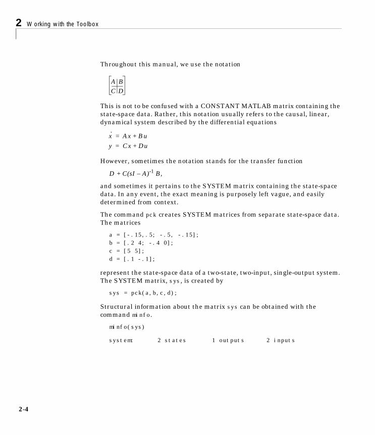
Throughout this manual, we use the notation
This is not to be confused with a CONSTANT MATLAB matrix containing thestate-space data. Rather, this notation usually refers to the causal, linear,dynamical system described by the differential equations
However, sometimes the notation stands for the transfer function
D + C(sI – A)-1 B,
and sometimes it pertains to the SYSTEM matrix containing the state-spacedata. In any event, the exact meaning is purposely left vague, and easilydetermined from context.
The command pck creates SYSTEM matrices from separate state-space data.The matrices
a = [-.15,.5; -.5, -.15]; b = [.2 4; -.4 0]; c = [5 5]; d = [.1 -.1];
represent the state-space data of a two-state, two-input, single-output system.The SYSTEM matrix, sys, is created by
sys = pck(a,b,c,d);
Structural information about the matrix sys can be obtained with thecommand minfo.
minfo(sys)
system: 2 states 1 outputs 2 inputs
A BC D
x· Ax Bu+=
y Cx Du+=

The Data Structures
The command unpck extracts the a, b, c, and d matrices from a SYSTEMmatrix. You can also examine the contents of the a, b, c, and d matrices withoutexplicitly forming them as new variables. Use the command see for thispurpose.
see(sys)
A matrix
press any key to move to B matrix
B matrix
press any key to move to C matrix
C matrix
press any key to move to D matrix
D matrix
The commands minfo and see work on any of the µ-Tools data structures.The command pss2sys converts CONSTANT matrix data in packed form,[A B; C D], into a µ-Tools SYSTEM matrix. The command sys2psstransforms a SYSTEM matrix in a packed CONSTANT matrix.Alternatively, you can generate a purely random SYSTEM matrix with thecommand sysrand by specifying its number of states, inputs and outputs.
The command spoles finds the eigenvalues of the A matrix of a SYSTEMmatrix. The transmission zeros are calculated using szeros. In this example,sys has no transmission zeros. A formatted display of the system poles isproduced with the µ-Tools command rifd.
-0.1500 0.5000
-0.5000 -0.1500
-0.2000 4.0000
-0.4000 0
5 5
-0.1000 -0.1000
2-5

2 Working with the Toolbox
2-6
spoles(sys) ans =
rifd(spoles(sys))
SYSTEM matrices can easily be interconnected (cascade, parallel, feedback) togive new SYSTEM matrices. See “Interconnecting Matrices” for moreinformation.
VARYING MatricesMatrix-valued functions of a single, independent real variable are common insystems theory. VARYING matrices The frequency response of amultiple-input, multiple-output (MIMO) system is a good example of such afunction. The independent variable is frequency, and at each frequency thetransfer function between the inputs and the outputs is a complex matrix.represents these types of matrix functions with a data structure called aVARYING matrix.
In general, suppose G is a matrix-valued function of a single real variable
. One method to store this function on the computer is to evaluatethe function G at N discrete values of , call them x1,x2,. . .,xN and store allof the evaluations. This is the approach taken by µ-Tools.
Consider a simple example:
mat1 = [.1 -.1;.25.5]; iv1 = 0; mat2 = 2*mat1;iv2 = 1; mat3 = 2*mat2; iv3 = 2;
–0.1500 + 0.5000i
–0.1500 – 0.5000i
real imaginary frequency damping
–1.5000e-01 –5.0000e-01 5.2202e–01 2.8735e–01
–1.5000e-01 5.0000e–01 5.2202e–01 2.8735e–01
G:R Cn m×→x R∈

The Data Structures
The command vpck creates the VARYING matrix data structure from columnstacked matrix and independent variable data. This is done as follows:
matdata = [mat1; mat2; mat3]; ivdata = [iv1; iv2; iv3]; vmat = vpck(matdata,ivdata)
minfo displays structural characteristics of the matrix and displays the data:
minfo(vmat)
varying: 3 pts 2 rows 2 cols
see(vmat)
2 rows 2 columns
iv = 0
iv = 1
iv = 2
Note that variable name iv stands for independent variable in the abovedisplay. The command seeiv displays only the independent variable values ofthe VARYING matrix vmat:
seeiv(vmat)
Analogous to vpck the command vunpck unpacks the matrix data andindependent variable data from a VARYING matrix.
Several commands allow manipulation of the matrix and independent variabledata. tackon simply appends one VARYING matrix to another (both must have
0.1000 –0.1000
0.2500 0.5000
0.2000 –0.2000
0.5000 1.0000
0.4000 –0.4000
1.0000 2.0000
2-7
2 Working with the Toolbox
2-8
the same number of rows and columns in the matrix data). This destroys anysequential properties of the independent variable data; i.e., the data will not bein monotonically increasing order. sortiv reorders the matrices within aVARYING matrix so that the independent variables are increasing (ordecreasing).
All of the information about the structure is contained in a single MATLABmatrix, hence functions returning single matrices can be nested. Hence,sophisticated manipulations can be formed as single line commands. Forexample, to merge two VARYING matrices and reorder the independentvariable’s values, use the command sortiv(tackon(vmat1,vmat2)).
CONSTANT MatricesIf a MATLAB variable is neither a SYSTEM nor a VARYING matrix it istreated by µ-Tools as a CONSTANT matrix. CONSTANT matricesCONSTANT matrices can be arguments to functions that normally expectVARYING or SYSTEM matrix arguments.
The treatment of CONSTANT matrices is consistent with that of a constantgain linear system. In operations normally performed on SYSTEM matrices,the CONSTANT matrix is analogous to a linear system with only a D matrix.In operations where a VARYING interpretation is required, the CONSTANTmatrix is assumed to be constant across all values of the independent variable.This is consistent with the frequency response (or step response) of a constantgain linear system.
AcknowledgmentsThe data structures used in are based on the following paper:
Stein, Gunter, and Stephen Pratt, “LQG Multivariable Design Tools,” AGARDLecture Series No 117, Multi-variable Analysis and Design Techniques,September 1981.

Accessing Parts of Matrices
Accessing Parts of MatricesThe SYSTEM matrix and VARYING matrix data structures allow a largeamount of data to be stored in a single MATLAB entity. It is often necessary todisplay or operate on only a part of that data.
The command sel creates subsystems from VARYING, SYSTEM, orCONSTANT matrices. The subsystem rows (or outputs) and columns (orinputs) are specified. Conceptually, the options are
lcl subvmat = sel(vmat,rows,columns); subconst = sel(const,rows,columns); subsyst = sel(syst,outputs,inputs);
For example,
subvmat = sel(vmat,1:2,2); minfo(subvmat)
varying: 3 pts 2 rows 1 cols
selects rows 1 and 2 and column 2 from each matrix in vmat. You can use theMATLAB colon notation in the specification of the rows and columns. To selectall rows or columns, use the character string ':' in single quotes. When sel isused on a SYSTEM matrix, only the dimensions of the B, C, and D matriceschange. All the states remain, which may result in a (non)minimal system.Extra states of the system can be removed by performing a balanced realization(sysbal) or with the commands strunc and sresid.
For VARYING matrices you can access a portion of the independent variableswith the command xtract. For example,
vmat2 = xtract(vmat,0.5,1.5);
2-9

2 Working with the Toolbox
2-1
selects the matrices in vmat with independent variables between 0.5 and 1.5.In this case it is a VARYING matrix with a single data point.
see(vmat2)
2 rows 2 columns
iv = 1
A VARYING matrix can be converted to a CONSTANT matrix via thecommand var2con.
The command xtracti extracts (as a VARYING matrix) the data byindependent variable index, rather than by independent variable value. As inthe case of xtract, xtracti returns a VARYING matrix.
0.2000 –0.2000
0.5000 1.0000
0

Interconnecting Matrices
Interconnecting Matricesµ-Tools provides several functions for connecting matrices together. All of thefunctions described here work with interconnections of SYSTEM andCONSTANT matrices or VARYING and CONSTANT matrices. If the matricesrepresented are consistent, the combination is allowed. The interconnection ofa SYSTEM and a VARYING matrix is not allowed in µ-Tools (actually it isallowed — see veval for examples of VARYING SYSTEM matrices).
The commands madd, msub, and mmult perform the appropriate arithmeticoperations on the matrices. A block diagram representation is shown in thefollowing figure.
Note that for multivariate matrices, the order of the arguments is important.In the VARYING matrix case, the arithmetic operations are performedmatrix-by-matrix, for each value of the independent variable. The followingexample illustrates this:
A two-row and one-column VARYING matrix, vmat3, is constructed with threeindependent variables values.
vmat3 = vpck([2 2 4 4 8 8]',[0 1 2]'); minfo(vmat3)
varying: 3 pts2 rows1 cols
madd(mat1,mat2)
mat2
mat1
6
? h+
mmult(mat1,mat2)
mat2mat1
2-11

2 Working with the Toolbox
2-1
The VARYING matrix vmat3 is multiplied by vmat to form vmat4 and the valueof the resulting matrix at the independent variables between 0 and 0.5 aredisplayed.
vmat4 = mmult(vmat,vmat3); minfo(vmat4) 60.23in
varying: 3 pts 2 rows 1 cols
see(xtract(vmat4,0,0.5))
2 rows 1 column
iv = 00
1.5000
Each matrix in vmat is 2 × 2. Each matrix in vmat3 is 2 × 1, and so themultiplication results in each matrix of vmat4 being 2 × 1. Commands madd,msub, and mmult allow up to nine matrices of compatible dimensions to beadded, subtracted or multiplied simultaneously by including them as inputarguments. When interconnecting VARYING matrices with any of thecommands in this section, a check is made to verify that each matrix has thesame independent variable values. If not, an error is returned.
There are additional commands for combining matrices: abv, daug, and sbs.These can be interpreted as placing matrices above one another, diagonalaugmentation of matrices, and placing matrices side-by-side, as shown in thefollowing figure.
abv(top,bot)
bot
top
daug(ul,lr)
ul
lr
sbs(left,right)
right
left
6h+
2
Interconnecting Matrices
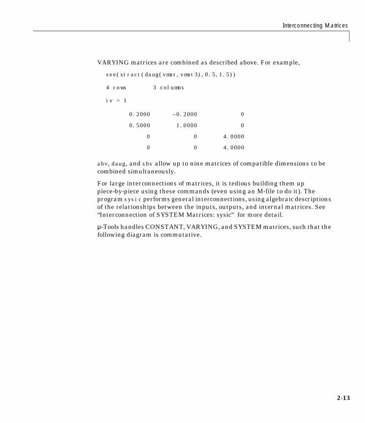
VARYING matrices are combined as described above. For example,
see(xtract(daug(vmat,vmat3),0.5,1.5))
4 rows 3 columns
iv = 1
abv, daug, and sbs allow up to nine matrices of compatible dimensions to becombined simultaneously.
For large interconnections of matrices, it is tedious building them uppiece-by-piece using these commands (even using an M-file to do it). Theprogram sysic performs general interconnections, using algebraic descriptionsof the relationships between the inputs, outputs, and internal matrices. See“Interconnection of SYSTEM Matrices: sysic” for more detail.
µ-Tools handles CONSTANT, VARYING, and SYSTEM matrices, such that thefollowing diagram is commutative.
0.2000 –0.2000 0
0.5000 1.0000 0
0 0 4.0000
0 0 4.0000
2-13

2 Working with the Toolbox
2-1
Consider beginning in the upper-right corner (individual systems of SYSTEMand CONSTANT matrices) and proceeding to the lower left corner (a singleVARYING matrix). The result will be independent of the path taken. This isbecause in linear systems, the frequency response of an interconnection is thealgebraic interconnection of the individual frequency responses. However, dueto numerical roundoff, the calculations actually are not commutative, andthere may be small differences between the two results. For example, it issometimes numerically better to interconnect the frequency response of twosystems rather than interconnect the two systems and then take theirfrequency response. This can be true when there are a large number of statesin the interconnection structure.
Interconnections involving feedback are performed with sysic, described in“Interconnection of SYSTEM Matrices: sysic” . The basic feedback loopinterconnection program used by sysic is called starp, and is described inChapter 4, “µ-Tools Commands for LFTs” on page 4-10.
The commands (sbs, mmult, starp, etc.) to form the interconnection step areidentical whether you are dealing with VARYING or SYSTEMrepresentations.
System
Combined
ARYING M t i
System
Combined
Systems
Individual
Systems
Individual
SYSTEM, CONSTANT
Matrices
? ?
Interconnect
Interconnect
Frequency
Response
Frequency
Response
4
Plotting VARYING Matrices
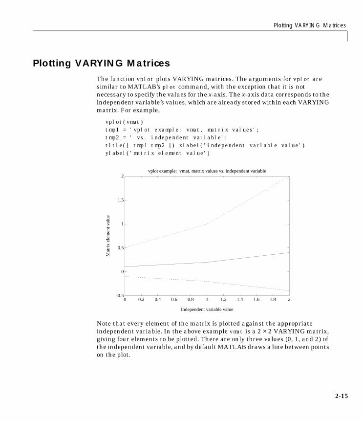
Plotting VARYING Matrices The function vplot plots VARYING matrices. The arguments for vplot aresimilar to MATLAB’s plot command, with the exception that it is notnecessary to specify the values for the x-axis. The x-axis data corresponds to theindependent variable’s values, which are already stored within each VARYINGmatrix. For example,
vplot(vmat) tmp1 = 'vplot example: vmat, matrix values'; tmp2 = ' vs. independent variable'; title([ tmp1 tmp2 ]) xlabel('independent variable value') ylabel('matrix element value')
Note that every element of the matrix is plotted against the appropriateindependent variable. In the above example vmat is a 2 × 2 VARYING matrix,giving four elements to be plotted. There are only three values (0, 1, and 2) ofthe independent variable, and by default MATLAB draws a line between pointson the plot.
-0.5
0
0.5
1
1.5
2
0 0.2 0.4 0.6 0.8 1 1.2 1.4 1.6 1.8 2
vplot example: vmat, matrix values vs. independent variable
Independent variable value
Mat
rix e
lem
ent v
alue
2-15
2 Working with the Toolbox
2-1
In the MATLAB plot command, different axis types are accessed by differentfunctions, loglog, semilogx, and others. In vplot the axis type is set by anoptional string argument. The default, used in the above example, is a linear/linear scale. The generic vplot function call looks like
vplot('axistype',vmat1,'linetype1',vmat2,'linetype2',...)
The axistype argument, a character string, allows the specification oflogarithmic or linear axes as well as: magnitude, log magnitude, and phase.There are also some control-specific options: bode, nyq, and nic, which specifyBode, Nyquist, and Nichols plots, respectively. The complete range of choices isnot demonstrated here. Refer to vplot in the Chapter 8, “Reference”, for moredetails. Subsequent sections introduce additional control-oriented examplesand demonstrate other options in vplot.
The linetype arguments are optional and are identical to those in theMATLAB plot command.
An important feature of vplot is its ability to plot multiple VARYING matriceson the same plot without having to have the same independent variables. Avmat argument may be a CONSTANT. In this case the value of theCONSTANT is plotted over all independent variables. This is consistent withthe interpretation given to CONSTANT matrices in the interconnection ofsystems. Hence a CONSTANT matrix would appear as a horizontal line on theplot. This is to be contrasted with a VARYING matrix containing only one datapoint, which would appear as a single point on the plot.
Consider the following example where vmat2 is a VARYING matrix with onlyone independent variable value (ie., one data point). The constant pi/2 is alsoplotted.
vplot(vmat,'r-',vmat2,'g*',pi/2,'b-.') title('vplot example: VARYING and CONSTANT matrices')xlabel('Independent variable value') ylabel('Matrix element value')
6

Plotting VARYING Matrices
-0.5
0
0.5
1
1.5
2
0 0.2 0.4 0.6 0.8 1 1.2 1.4 1.6 1.8 2
**
**
**
**
vplot example: VARYING and CONSTANT matrices
Independent variable value
Mat
rix e
lem
ent v
alue
2-17
2 Working with the Toolbox
2-1
VARYING Matrix Functions Many of the MATLAB matrix functions have analogous µ-Tools functions thatoperate on VARYING matrices. These operations are performed on amatrix-by-matrix basis for every submatrix associated with an independentvariable value within the VARYING matrix. If a CONSTANT matrix is theargument of these functions, the operation is identical to the correspondingMATLAB function. These functions are:
The functions veval and vebe perform a named operation on VARYINGmatrices. vebe performs MATLAB or user-defined functions on the elements ofa VARYING matrix (for example: sin, tan. . .). veval operates on the entireVARYING matrix and can perform any function including those with multipleinput and output arguments. vebe and veval allow the evaluation of anyMATLAB matrix function on VARYING matrices. The following exampleshows a VARYING matrix with only one independent variable value forbrevity:
minfo(vmat2)
varying: 1 pts 2 rows 2 cols
see(veval('sin',vmat2))2 rows 2 columnsiv = 1
vmat2dat = var2con(vmat2);sin(vmat2dat)
ans =
vabs vceil vdet vdiag veig
veval vexpm vfloor vinv vimag
vnorm vpinv vpoly vrcond vreal
vroots vschur vsvd
0.1987 –0.1987
0.4794 0.8415
0.1987 –0.1987
0.4794 0.8415
8
VARYING Matrix Functions
vebe('sqrt',sin(vmat2dat))ans =
All arithmetic operations can be performed on VARYING matrices, sometimeswith a built-in µ-Tools function, and sometimes resorting to veval. Thefollowing table summarizes some standard operation.
In each case, veval could have been used. However, veval can be quite slow,since it is essentially a for loop of eval commands. For that reason, somespecific commands (madd, mmult, vldiv, etc.) are provided. The complete set ofVARYING operations should allow you to write algorithms more easily usingthe data structures in µ-Tools.
0.4458 0 + 0.4458i
0.6924 0.9173
MATLAB Matrix Function µ-Tools VARYING Function
A + B +...+ H madd(A,B,...,H)
A – B –...– H msub(A,B,...,H)
A * B *...* H mmult(A,B,...,H)
A / B vrdiv(A,B)
A \ B vldiv(A,B)
A .* B veval('.*',A,B)
A ./ B veval('./',A,B)
A ^ b veval('^',A,b)
A .^b veval('.^',A,b)
A' cjt(A)
A.' transp(A)
conj(A) cj(A)
sin(A) vebe('sin',A)
2-19

2 Working with the Toolbox
2-2
More Sophisticated SYSTEM Functions
Frequency Domain FunctionsThe command frsp calculates frequency responses of SYSTEM matrices. Youcan specify the frequencies at which the response is to be evaluated via theMATLAB logspace and linspace commands. These become the independentvariable values in the VARYING frequency response output.
Given an input vector of N real frequencies, omega = [ω1,. . .,ωN] and a SYSTEMmatrix sys, the µ-Tools command frsp,
sys_g = frsp(sys,omega)
calculates
C(jwiI – A)–1B + D, i = 1, . . ., N
for each independent variable wi and stores it in sys_g whose independentvariables are the N frequency points. You can specify a discrete-timeevaluation by specifying an optional sampling time, T. In this case each matrixin the VARYING output is
C(ejω,T I – A) B + D.
Consider a simple second order example. The function nd2sys creates theSYSTEM representation from numerator and denominator polynomials. In thefollowing example the system sys1 has the transfer function
0.5s– 1+
s2 0.2s 1+ +---------------------------------.
0

More Sophisticated SYSTEM Functions
The MATLAB command logspace can create a logarithmically spacedfrequency vector.
sys1 = nd2sys([-0.5,1],[1,0.2,1]); minfo(sys1)
system: 2 states 1 outputs 1 inputs
omega = logspace(-1,1,200); sys1g = frsp(sys1,omega); minfo(sys1g)
varying: 200 pts 1 rows 1 cols
vplot('bode',sys1g)
10-2
10-1
100
101
10-1 100 101
Log
Mag
nitu
de
Frequency (radians/sec)
-4
-2
0
2
4
10-1 100 101
Pha
se (
radi
ans)
Frequency (radians/sec)
2-21

2 Working with the Toolbox
2-2
You can transform sys1 to the digital domain via a prewarped Tustintransformation. The command tustin performs this function. In this examplea sample time of one second is used. The prewarping frequency is chosen as oneradian/second. For control purposes it is often better to choose the crossoverpoint as the prewarp frequency.
dsys1 = tustin(sys1,1,1); dsys1z = frsp(dsys1,omega,1); vplot('bode',sys1g,dsys1z)
Time Domain FunctionsTime responses of continuous systems are calculated with the function trsp.The required input arguments are the SYSTEM matrix and an input matrix.A discrete SYSTEM matrix is handled with the function dtrsp.
User-specified time functions can be created with the function siggen. siggencan create signals based on both random and deterministic functions. In this
10-4
10-3
10-2
10-1
100
101
10-1 100 101
Log
Mag
nitu
de
Frequency (radians/sec)
-4
-2
0
2
4
10-1 100 101
Pha
se (
radi
ans)
Frequency (radians/sec)
2

More Sophisticated SYSTEM Functions
example, siggen generates an input, u, to the system, sys1. Note how asaturation, in this case π, is implemented.
u = siggen('min(pi,sqrt(t)+0.25*rand(size(t)))',[0:.1:40]); y = trsp(sys1,u);
integration step size: 0.1
vplot(u,y) title('Response of sys1 (dashed) to input, u (solid)')xlabel('Time (seconds)')
trsp calculates a default step-size based on the minimum spacing in the inputvector and the highest frequency eigenvalue of the A matrix. For high ordersystems, we recommended you use some form of model reduction (see the“Model Reduction” section in Chapter 3) to remove high frequency modeswhich do not have a significant effect on the output.
-0.5
0
0.5
1
1.5
2
2.5
3
3.5
4
0 5 10 15 20 25 30 35 40
Response of sys1 (dashed) to input, u (solid)
Time (seconds)
2-23

2 Working with the Toolbox
2-2
trsp assumes that the input is constant between the values specified in theinput vector. The following example illustrates the consequences of thisassumption:
sys1a = pck(-1,1,1); minfo(sys)
system: 1 states 1 outputs 1 inputsu1a = vpck([0:10:50]',[0:10:50]'); y1a = trsp(sys1a,u1a,60);
integration step size: 0.1interpolating input vector (zero under hold)minfo(y1a)
varying: 601 pts 1 rows 1 colsvplot(u1a,'-.',y1a,'-') xlabel('Time: seconds') text(10,20,'input'), text(25,10,'output')
At first glance the output does not seem to be consistent with the plotted input.Remember that trsp assumes that the input is held constant between specifiedvalues. The vplot and plot commands display a linear interpolation betweenpoints. This can be seen by displaying the input signal interpolated to at least
0
5
10
15
20
25
30
35
40
45
50
0 10 20 30 40 50 60
Time: seconds
input
output
4

More Sophisticated SYSTEM Functions
as small a step-size as the default integration step (here 0.1 seconds). Theµ-Tools function vinterp performs zero-order hold or linear interpolation of theindependent variable.
vplot(u1a,'-.',vinterp(u1a,0.1),'--',y1a,'-') xlabel('Time: seconds') text(5,44,'dash-dot: input') text(5,40,'dashed: interpolated input') text(5,36,'solid: output')
The staircase nature of the input is now evident. To have a ramp input, you canuse the function vinterp to provide linear interpolation as shown by thefollowing example:
uramp = vinterp(u1a,0.1,60,1); minfo(uramp)
varying: 601 pts 1 rows 1 colsyramp = trsp(sys1a,uramp);
integration step size: 0.1vplot(uramp,'-.',yramp,'-') xlabel('Time: seconds') text(20,15,'output') text(12,20,'input')
0
5
10
15
20
25
30
35
40
45
50
0 10 20 30 40 50 60
Time: seconds
dash-dot: input
solid: output
dashed: interpolated input
2-25

2 Working with the Toolbox
2-2
Note that because the input is regularly spaced, with spacing less than or equalto the default integration time, trsp does not interpolate the input. No finaltime was specified in the trsp argument list. However 60 seconds was specifiedto vinterp as the final time, and this became the last time in the input vectoruramp.
To illustrate the use of dtrsp, a bilinear transformation generates a digitalsystem. The sample time is chosen as 1 second. The output is plotted against a1 second interpolation of the input.
T = 1; dsys1a = tustin(sys1a,T); ydig = dtrsp(dsys1a,u1a,T); vplot(ydig,'-',vinterp(u1a,1),'-.') xlabel('Time: seconds')
0
5
10
15
20
25
30
35
40
45
50
0 10 20 30 40 50 60
output
input
Time: seconds
6

More Sophisticated SYSTEM Functions
trsp can easily generate large VARYING matrices. If the independentvariables are more closely spaced than necessary for a good graphical display,you can use the µ-Tools function vdcmate to select every nth point from thefinal output.
Note that both vinterp and vdcmate have analogous Signal Processing Toolboxfunctions, interp and decimate, but do not function in the same manner.
Signal Processing and IdentificationThe µ-Tools VARYING data structure provides a convenient means of storinglarge amounts of experimental data in a single MATLAB matrix. To use this inidentification experiments, routines have been provided to perform FastFourier Transforms (FFTs) and inverse FFTs for VARYING matrices. Thefunctions are vfft and vifft, respectively. These routines call the appropriateMATLAB fft and ifft routines to perform the FFT calculations and have thesame function arguments as those for fft and ifft.
Note that the FFTs performed are one dimensional, irrespective of the row andcolumn dimensions of the VARYING matrix. The independent variable is usedas the index in the FFT. Consequently xfreq = vfft(xtime) works if xtime isa VARYING matrix with row and column dimensions greater than one. Theresult, xfreq, is a VARYING matrix of the same size and has the same number
0
5
10
15
20
25
30
35
40
45
50
0 10 20 30 40 50 60
Time: seconds
2-27

2 Working with the Toolbox
2-2
of independent variables. The independent variables of xtime are assumed tobe time in seconds. xfreq is returned with frequency (in radians/second) as theindependent variable.
In the following example a random signal is passed through a single-input,two-output system and FFTs of the outputs are performed with a single vfftfunction. The sample frequency is 10 Hz, with a foldover frequency of 10πradians/second. This may be hard to distinguish on the log-log plot. Outputtime history plots are shown in Figure 2-1 and their FFTs are shown in Figure2-2.
time = [0:0.1:102.3]'; u1 = siggen('rand(size(t)) - 0.5',time); sys2 = nd2sys(1,[5,1]); sys3 = abv(sys1,sys2); y1 = trsp(sys3,u1);
integration step size: 0.1minfo(y1)
varying: 1024pts 2 rows 1 colsvplot(y1) title('Response of sys3 (solid) to input u1 (dashed)') xlabel('Time: seconds')
y1f = vfft(y1); minfo(y1f)
varying:1024pts2 rows 1 colsvplot('liv,lm',y1f) z='Fast Fourier Transform magnitude of sys3 response: y1'; title([ z ]) xlabel('Frequency: radians/second') ylabel('Magnitude')
Warning: Data includes a number that is negative or zero. The LOG of hits results in NaN or Infinity and is not shown on plot.
8

More Sophisticated SYSTEM Functions
Figure 2-1 System Response Time Histories
Figure 2-2 FFTs of the Output
-0.4
-0.3
-0.2
-0.1
0
0.1
0.2
0.3
0.4
0.5
0 20 40 60 80 100 120
response of sys3 (solid) to input u1 (dashed)
Time: seconds
10-3
10-2
10-1
100
101
102
103
10-2 10-1 100 101 102
Fast Fourier Transform magnitude of sys3 response: y1
Frequency: radians/second
Mag
nitu
de
2-29

2 Working with the Toolbox
2-3
The µ-Tools function vplot displays this warning message since there is a datavalue at zero frequency that cannot be plotted on the log frequency scale.
The Signal Processing Toolbox provides a means of performing spectralanalysis with the function spectrum. The µ-Tools function vspect operates ina similar manner on VARYING matrices. Given a signal x and a signal y,vspect can calculate the power spectral density of x (Pxx), the power spectraldensity of y (Pyy), the cross spectral density (Pxy), the transfer function from xto y (Txy), and the coherence (Cxy). The VARYING matrix result will have thefollowing five columns, [Pxx, Pyy, Pxy, Txy, Cxy]. The command vspect(x,m) willcalculate the power spectral density of each element of the VARYING matrix,x, using averaged FFTs of length m. The algorithm is exactly that used forspectrum. See the Signal Processing Toolbox for further information.
The calculation of transfer functions using vspect restricts the input x to be aone-by-one VARYING matrix and the outputs y to be an nr × 1 VARYINGmatrix. This corresponds to being able to do single-input, multiple-output(SIMO) identification experiments for a system with nr outputs. Each row ofthe result then corresponds to an output or its associated SISO transferfunction. The calling sequence for vspect is vspect(x,y,m).
In the following example, vspect estimates the single-input, two-outputtransfer function from the data generated in the previous example. A smallamount of random noise is added to the output, y1, to make the problem morerealistic. 512 point FFTs are applied to the data with an overlap of 256 points.An optional Hamming window, the fifth input argument, is used on the data inconjunction with the FFTs. The fourth column of the output is the estimatedtransfer function, which is displayed in Figure 2-3 using the sel function.
noise1 = siggen('0.05*(rand(2,1)-[0.5;0.5])',time); y1meas = madd(y1,noise1); P1 = vspect(u1,y1,512,256,'hamming');3 hamming windows in averaging calculationminfo(P1)
varying: 256 pts 2 rows 5 colsvplot('bode',sel(P1,[1:2],4),'-',frsp(sys3,omega),'-.') tmp1 = 'sys3 (dash-dot) and estimated'; tmp2 = ' transfer function (solid)'; title([ tmp1 tmp2 ])
0

More Sophisticated SYSTEM Functions
Figure 2-3 Estimated Transfer Functions of the System
The command fitsys can be used to construct a state-space realization of theestimated transfer function data. The first input argument to fitsys is thefrequency response data as a VARYING matrix. This argument, frdata, canhave dimension of a single-input/multi-output or multiple-input/single-outputVARYING matrix. The second input argument, ord, is the state-order of thedesired fit. The third input argument, weight is a weighting matrix with thesame independent variable values as frdata. The fourth input argument, code,can be set to restrict the curve fitting algorithm to stable transfer functions.The default value for weight is 1, and the default value of code is 0, placing norestriction on the location of the rational fit’s poles. The output of fitsys is theSYSTEM sys. The state-order of sys is ord.
In this example fit the single-input, two-output estimated transfer functiondata with a third order model. Recall that the fourth column of P is theestimated transfer function data. We will restrict the fitting algorithm toconsider only frequency points between 0.1 rad/sec and 10 rad/sec. A plot of theestimated transfer function data and the third order model, sysord3, is shownin Figure 2-4. Notice that the poles of sysord3 are very close to the poles ofsys3, which was used to create the estimated transfer function data.
10-3
10-2
10-1
100
101
10-1 100 101 102
Log
Mag
nitu
de
Frequency (radians/sec)
-4
-2
0
2
4
10-1 100 101 102
Pha
se (
radi
ans)
Frequency (radians/sec)
sys3 (dash-dot) and estimated transfer function (solid)
2-31

2 Working with the Toolbox
2-3
estdata = sel(P1,[1:2],4); sysord3 = fitsys(xtract(estdata,0.1,10),3); vplot('bode',estdata,'-',frsp(sysord3,estdata),'-.') tmp1 = 'sysord3 (dashed) and estimated'; tmp2 = ' transfer function (solid)'; title([ tmp1 tmp2 ]) rifd(spoles(sysord3))
rifd(spoles(sys3))
real imaginary frequency damping
–3.1841e–01 –0.0000e+00 3.1841e–01 1.0000e+00
–1.1555e-01 –9.8732e–01 9.9406e–01 1.1624e–01
–1.1555e-01 9.8732e–01 9.9406e–01 1.1624e–01
real imaginary frequency damping
–2.0000e–01 0.0000e+00 2.0000e–01 1.0000e+00
1.0000e–01 –9.9499e–01 1.0000e+00 1.0000e–01
–1.0000e–01 9.9499e–01 1.0000e+00 1.0000e–01
2

More Sophisticated SYSTEM Functions
Figure 2-4 Estimated Transfer Functions and Third Order Model
101
100
101
102
400
200
0
Pha
se (
degr
ees)
Frequency (radians/sec)
101
100
101
102
104
102
100
102
Log
Mag
nitu
de
Frequency (radians/sec)
sysord3 (dashed) and estimated transfer function (solid)
2-33

2 Working with the Toolbox
2-3
Interconnection of SYSTEM Matrices: sysic µ-Tools has a simple linear interconnection program called sysic. sysic formslinear interconnections of CONSTANT and SYSTEM matrices (or CONSTANTand VARYING matrices) simply by calculating the loop equations of theinterconnection.
Using sysic involves setting up several variables in the MATLAB workspace,and then running the script-file sysic. The defined variables delineate thedetails of the interconnection.
In order to explain the meaning of the sysic commands, consider a three-input,two-output SYSTEM matrix T,
which has internal structure
T
noise
deltemp
setpoint
y1
y2
k
pact
wt57.3
setpoint
g+
+6noise
deltempy1
y2
-
-
6
g
+
4
Interconnection of SYSTEM Matrices: sysic
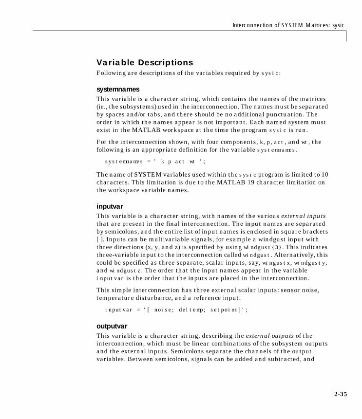
Variable DescriptionsFollowing are descriptions of the variables required by sysic:
systemnamesThis variable is a character string, which contains the names of the matrices(ie., the subsystems) used in the interconnection. The names must be separatedby spaces and/or tabs, and there should be no additional punctuation. Theorder in which the names appear is not important. Each named system mustexist in the MATLAB workspace at the time the program sysic is run.
For the interconnection shown, with four components, k, p, act, and wt, thefollowing is an appropriate definition for the variable systemnames.
systemnames = ' k p act wt ';
The name of SYSTEM variables used within the sysic program is limited to 10characters. This limitation is due to the MATLAB 19 character limitation onthe workspace variable names.
inputvarThis variable is a character string, with names of the various external inputsthat are present in the final interconnection. The input names are separatedby semicolons, and the entire list of input names is enclosed in square brackets[ ]. Inputs can be multivariable signals, for example a windgust input withthree directions (x, y, and z) is specified by using windgust3. This indicatesthree-variable input to the interconnection called windgust. Alternatively, thiscould be specified as three separate, scalar inputs, say, wingustx, windgusty,and windgustz. The order that the input names appear in the variableinputvar is the order that the inputs are placed in the interconnection.
This simple interconnection has three external scalar inputs: sensor noise,temperature disturbance, and a reference input.
inputvar = '[ noise; deltemp; setpoint]';
outputvarThis variable is a character string, describing the external outputs of theinterconnection, which must be linear combinations of the subsystem outputsand the external inputs. Semicolons separate the channels of the outputvariables. Between semicolons, signals can be added and subtracted, and
2-35

2 Working with the Toolbox
2-3
multiplied by scalars. For multivariable subsystems, arguments withinparentheses specify which subsystem outputs to use and in what order. Forinstance, plant(2:5,8,1,9:11) specifies outputs 2, 3, 4, 5, 8, 1, 9, 10, 11 from the system plant. If no arguments are specified with a system, then itis assumed that all outputs are being used, and in the order they appear in thatsystem.
In this example, the two outputs of the interconnection consist of the firstoutput of the plant (scaled by 57.3 to change units from radians to degrees)along with a tracking error, which is the difference between the setpoint inputand the second plant output.
outputvar = '[ 57.3*p(1); setpoint – p(2) ]';
input_to_sysThis variable denotes the inputs to a specific system. Each subsystem namedin the variable systemnames must have a variable set to define the inputs to thesubsystem. If the system name is controller, then call the variable that mustbe set using input_to_controller. Specify it in the same manner that thevariable outputvar is set, with inputs consisting of linear combinations ofsubsystem outputs and external inputs. Separate channels are separated bysemicolons, and the order of the inputs in the variable should match the orderof the inputs in the system itself.
Corresponding to the systemnames variable set above, there are four input_to_ statements required, which are
input_to_k = '[ noise + p(2); setpoint ]'; input_to_act = '[ k ]'; input_to_wt = '[ deltemp ]'; input_to_p = '[ wt; act ]';
This means that the input to the controller consists of the sensor noise plus thesecond output of the plant, and the reference input. The input to the actuatoris the output of the controller. The input to the weighting function is thetemperature disturbance, and the input to the plant consists of the output ofthe weighting function, followed by the output of the actuator.
sysoutnameThis character string variable is optional. If it exists in the MATLABworkspace when sysic is run, the interconnection that is created by sysic is
6

Interconnection of SYSTEM Matrices: sysic
placed in a MATLAB variable whose name is given by the string insysoutname. If this variable does not exist in the workspace, then theinterconnection is automatically placed in the variable ic_ms.
The command line
sysoutname = 'T';
will cause sysic to store the final interconnection in a SYSTEM matrix called T.
cleanupsysicThis variable is used to clean up the workspace. After running sysic, all of theabove variables that describe the interconnection are left in the workspace.These will be automatically cleared if the optional variable cleanupsysic is setto the character string yes. The default value of the variable is no, which doesnot result in any of the user-defined sysic descriptions being cleared. TheMATLAB matrices listed in the variable systemnames are never automaticallycleared.
Running sysicIf the variables systemnames, inputvar, and outputvar are set, and for eachname name_i appearing in systemnames, the variable input_to_name_i is set,then the interconnection is created by running the M-file sysic. Depending onthe existence/nonexistence of the variable sysoutname, the resultinginterconnection is stored in a user-specified MATLAB variable or the defaultMATLAB variable ic_ms.
Within sysic, error-checking of the consistency and availability of subsystemmatrices and their inputs aid in debugging faulty sysic interconnectiondescriptions.
The input/output dimensions of the final interconnection are defined byinputvar and outputvar variables.
Returning to the initial example, the following sysic commands were used togenerate the three-input, two-output SYSTEM matrix clp. (Note that thedimensions of the variables k, p, act, and wt must be consistent with theproblem description.)
2-37

2 Working with the Toolbox
2-3
systemnames = ' k p act wt '; inputvar = '[ noise; deltemp; setpoint]'; outputvar = '[ 57.3*p(1); setpoint - p(2) ]'; input_to_k = '[ noise + p(2); setpoint ]'; input_to_act = '[ k ]'; input_to_wt = '[ deltemp ]'; input_to_p = '[ wt; act ]'; sysoutname = 'clp'; cleanupsysic = 'yes'; sysic;
The syntax of sysic is limited, and for the most part restricted to what isshown here. Some additional features are illustrated in the more complicateddemonstration problems.
HIMAT Design ExampleThe HIMAT example provides another example of how to constructinterconnection systems from block diagram descriptions. The HIMAT plantmodel is described in more detail in the section, “HIMAT Robust PerformanceDesign Example” in Chapter 7. The interconnection diagram shown in Figure2-5 corresponds to the HIMAT design example.
Figure 2-5 HIMAT Interconnection
Given that there are four SYSTEM matrices, named himat, wdel, wp, and k, inthe MATLAB workspace, each with two inputs and two outputs, the following10 lines form the sysic commands to make the interconnection structureshown below, which is placed in the variable clp. These can be executed at the
8
Interconnection of SYSTEM Matrices: sysic
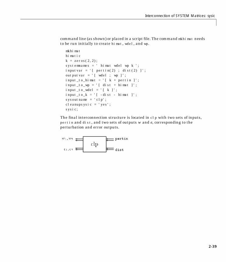
command line (as shown) or placed in a script file. The command mkhimat needsto be run initially to create himat, wdel, and wp.
mkhimat himatic k = zeros(2,2); systemnames = ' himat wdel wp k '; inputvar = '[ pertin(2) ; dist(2) ]'; outputvar = '[ wdel ; wp ]'; input_to_himat = '[ k + pertin ]'; input_to_wp = '[ dist + himat ]'; input_to_wdel = '[ k ]'; input_to_k = '[ -dist - himat ]'; sysoutname = 'clp'; cleanupsysic = 'yes'; sysic;
The final interconnection structure is located in clp with two sets of inputs,pertin and dist, and two sets of outputs w and e, corresponding to theperturbation and error outputs.
clppertin
dist
w1; w2
e1; e2
2-39

2 Working with the Toolbox
2-4
0
3
H∞ Control andModel Reduction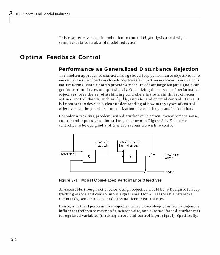
3 H∞ Control and Model Reduction
3-2
This chapter covers an introduction to control analysis and design,sampled-data control, and model reduction.
Optimal Feedback Control
Performance as Generalized Disturbance RejectionThe modern approach to characterizing closed-loop performance objectives is tomeasure the size of certain closed-loop transfer function matrices using variousmatrix norms. Matrix norms provide a measure of how large output signals canget for certain classes of input signals. Optimizing these types of performanceobjectives, over the set of stabilizing controllers is the main thrust of recentoptimal control theory, such as L1, H2, and H∞, and optimal control. Hence, itis important to develop a clear understanding of how many types of controlobjectives can be posed as a minimization of closed-loop transfer functions.
Consider a tracking problem, with disturbance rejection, measurement noise,and control input signal limitations, as shown in Figure 3-1. K is somecontroller to be designed and G is the system we wish to control.
Figure 3-1 Typical Closed-Loop Performance Objectives
A reasonable, though not precise, design objective would be to Design K to keeptracking errors and control input signal small for all reasonable referencecommands, sensor noises, and external force disturbances.
Hence, a natural performance objective is the closed-loop gain from exogenousinfluences (reference commands, sensor noise, and external force disturbances)to regulated variables (tracking errors and control input signal). Specifically,
H∞
K G
-reference - - -
? noise
-
?
6controlinput
external forcedisturbance
-trackingerror
e
e
Optimal Feedback Control
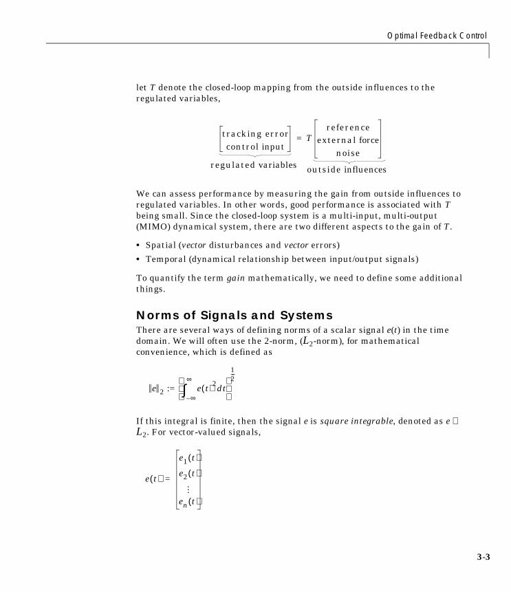
let T denote the closed-loop mapping from the outside influences to theregulated variables,
We can assess performance by measuring the gain from outside influences toregulated variables. In other words, good performance is associated with Tbeing small. Since the closed-loop system is a multi-input, multi-output(MIMO) dynamical system, there are two different aspects to the gain of T.
• Spatial (vector disturbances and vector errors)
• Temporal (dynamical relationship between input/output signals)
To quantify the term gain mathematically, we need to define some additionalthings.
Norms of Signals and SystemsThere are several ways of defining norms of a scalar signal e(t) in the timedomain. We will often use the 2-norm, (L2-norm), for mathematicalconvenience, which is defined as
If this integral is finite, then the signal e is square integrable, denoted as e ∈ L2. For vector-valued signals,
tracking errorcontrol input
Treference
external forcenoise
=
regulated variables outside influences
e 2 := e t( )2 td∞–
∞
∫
12---
e t( )
e1 t( )
e2 t( )
en t( )
=
…
3-3

3 H∞ Control and Model Reduction
3-4
the 2-norm is defined as
In µ-Tools the dynamical systems we deal with are exclusively linear, withstate-space model
or, in the transfer function form
e(s) = T(s)d(s), T(s) := C(sI – A)–1B + D
Two mathematically convenient measures of the transfer matrix T(s) in thefrequency domain are the matrix H2 and H∞ norms,
where the Frobenious norm (see the MATLAB norm command) of a complexmatrix M is
Both of these transfer function norms have input/output time-domaininterpretations. If, starting from initial condition x(0) = 0, two signals d and eare related by
eT
∞–
∞∫ t( )e t( )dt
12---
=
e 2 := e t( ) 22
∞–
∞∫ dt
12---
x·
e
A BC D
xd
=
T 2 :=1
2π------ T jω( ) F
2 dω∞–
∞
∫12---
T ∞:= maxσ T jω( )[ ]w R∈
M F := trace M*M( )
x·
e
A BC D
xd
=

Optimal Feedback Control
then
• for d, a unit intensity, white noise process, the steady-state variance of e is||T||2.
• The L2 (or RMS) gain from ,
is equal to ||T||∞. This is discussed in greater detail in the next section.
Using Weighted Norms to Characterize PerformanceIn any performance criterion, we must also account for
• Relative magnitude of outside influences
• Frequency dependence of signals
• Relative importance of the magnitudes of regulated variables
So, if the performance objective is in the form of a matrix norm, it shouldactually be a weighted norm
||WLTWR||
where the weighting function matrices WL and WR are frequency dependent, toaccount for bandwidth constraints and spectral content of exogenous signals.Within the structured singular value setting considered in Chapter 4, the mostnatural (mathematical) manner to characterize acceptable performance is interms of the MIMO ||⋅||∞ (H∞) norm. For this reason, we discuss someinterpretations of the H∞ norm.
Figure 3-2 Unweighted MIMO System
Suppose T is a MIMO stable linear system, with transfer function matrix T(s).For a given driving signal , define as the output, as shown in Figure 3-2.
d e→
maxe 2d 2
-----------d 0≠
T
~e ~d
d t( ) e
3-5
3 H∞ Control and Model Reduction
3-6
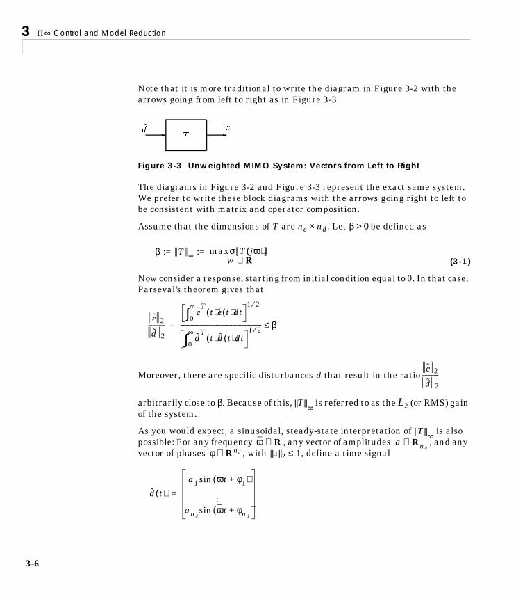
Note that it is more traditional to write the diagram in Figure 3-2 with thearrows going from left to right as in Figure 3-3.
Figure 3-3 Unweighted MIMO System: Vectors from Left to Right
The diagrams in Figure 3-2 and Figure 3-3 represent the exact same system.We prefer to write these block diagrams with the arrows going right to left tobe consistent with matrix and operator composition.
Assume that the dimensions of T are ne × nd. Let β > 0 be defined as
(3-1)
Now consider a response, starting from initial condition equal to 0. In that case,Parseval’s theorem gives that
Moreover, there are specific disturbances d that result in the ratio
arbitrarily close to β. Because of this, ||T||∞ is referred to as the L2 (or RMS) gainof the system.
As you would expect, a sinusoidal, steady-state interpretation of ||T||∞ is alsopossible: For any frequency , any vector of amplitudes , and anyvector of phases , with ||a||2 ≤ 1, define a time signal
T--~e~d
β := T ∞ := maxσ T jω( )[ ]w R∈
e 2
d 2-----------
eT
t( ) e t( ) td0
∞∫1 2⁄
dT
t( )d t( ) td0
∞∫
1 2⁄----------------------------------------------------- β≤=
e 2
d 2-----------
ω R∈ a Rnd∈
φ Rnd∈
d t( )a1 ωt φ1+( )sin
andωt φnd
+( )sin
=
…

Optimal Feedback Control
Applying this input to the system T results in a steady-state response of theform
The vector will satisfy ||b||2 ≤ β. Moreover, β, as defined in equation(3-1), is the smallest number such that this fact is true for every ||a||2 ≤ 1, , andφ.
Note that in this interpretation, the vectors of the sinusoidal magnituderesponses are unweighted, and measured in Euclidean norm. If realisticmultivariable performance objectives are to be represented by a single, MIMO||⋅||∞ objective on a closed-loop transfer function, additional scalings arenecessary. Since many different objectives are being lumped into one matrixand the associated cost is the norm of the matrix, it is important to usefrequency-dependent weighting functions, so that different requirements canbe meaningfully combined into a single cost function. Diagonal weights aremost easily interpreted.
Consider the diagram of Figure 3-4, along with Figure 3-2.
Assume that WL and WR are diagonal, stable transfer function matrices, withdiagonal entries denoted Li and Ri.
Figure 3-4 Weighted MIMO System
ess
ess t( )b1 ωt 1+( )sin
bneωt ne
+( )sin
= …
b Rne∈ω
WL
L1 0 … 0
0 L2 … 0
0 0 … Lne
=
…… …
...WR
R1 0 … 0
0 R2 … 0
0 0 … Rnd
=
…… …
...,
WL T WR
e d~d~e
e = WL~e = WLT~d = WLTWRd
3-7

3 H∞ Control and Model Reduction
3-8
Bounds on the quantity ||WLTWR||∞ will imply bounds about the sinusoidalsteady-state behavior of the signals and in Figure 3-2. Specifically,for sinusoidal signal , the steady-state relationship between , and||WLTWR||∞ is as follows: The steady-state solution , denoted as
(3-2)
satisfies for all sinusoidal input signals of the form
(3-3)
satisfying
if and only if ||WLTWR||∞ ≤ 1.
This approximately (very approximately — the next statement is not actuallycorrect) implies that ||WLTWR||∞ ≤ 1 if and only if for every fixed frequency ,and all sinusoidal disturbances of the form (3-3) satisfying
the steady-state error components will satisfy
d e(= Td)d e(= Td) d
ess
ess t( )e1 ωt 1+( )sin
eneωt nd
+( )sin
= …
ϕ
ϕ
WLijw( ) ei
21≤
i 1=
ne∑ d
d t( )d1 ωt φi+( )sin
dndωt φnd
+( )sin
= …
di2
WRijω( )
2---------------------------
i 1=
nd
∑ 1≤
ωd
di WRijω( )≤
ei1
WLijω( )
------------------------≤

Optimal Feedback Control
This shows how one could pick performance weights to reflect the desiredfrequency-dependent performance objective. Use WR to represent the relativemagnitude of sinusoids disturbances that might be present, and use torepresent the desired upper bound on the subsequent errors that are produced.
Remember, though, the weighted H∞ norm does not actually give element-by-element bounds on the components of based on element-by-elementbounds on the components of . The precise bound it gives is in terms ofEuclidean norms of the components of and (weighted appropriately byWL(j ) and WR(j )).
1WL---------
ed
e dω ω
3-9

3 H∞ Control and Model Reduction
3-1
Interconnection with Typical MIMO Performance ObjectivesThroughout this manual, we formulate closed-loop performance objectives asweighted closed-loop transfer functions which are to be made small throughfeedback. A generic example, which includes many relevant terms, is shown inblock diagram form in Figure 3-5. In the diagram, G denotes the plant modeland K is the feedback controller.
Figure 3-5 Generalized and Weighted Performance Block Diagram
The blocks in Figure 3-5 might be scalar (SISO) and/or multivariable (MIMO),depending on the specific example. The mathematical objective of H∞ controlis to make the closed-loop MIMO transfer function Ted satisfy ||Ted||∞ < 1. Theweighting functions are used to scale the input/output transfer functions suchthat when ||Ted||∞ < 1, the relationship between and is suitable.d e
0

Interconnection with Typical MIMO Performance Objectives
The interpretation of the signals, weighting functions and models are:
WcmdWcmd is used in problems requiring tracking of a reference command. Wcmdshapes (magnitude and frequency) the normalized reference command signalsinto the actual (or typical) reference signals that we expect to occur. It describesthe magnitude and the frequency dependence of the reference commandsgenerated by the normalized reference signal. Normally Wcmd is flat at lowfrequency and rolls off at high frequency. For example, in a flight controlproblem, fighter pilots can (and will) generate stick input reference commandsup to a bandwidth of about 2Hz. Suppose that the stick has a maximum travelof three inches. Pilot commands could be modeled as normalized signals passedthrough a first order filter
Signal Meaning
d1 Normalized reference command
Typical reference command
d2 Normalized exogenous disturbances
Typical exogenous disturbances
d3 Normalized sensor noise
Typical sensor noise
e1 Weighted control signals
Actual control signals
e2 Weighted tracking errors
Actual tracking errors
e3 Weighted plant errors
Actual plant errors
d1
d2
d3
e1
e2
e3
Wact3
12 2π⋅--------------s 1+---------------------------=
3-11

3 H∞ Control and Model Reduction
3-1
Wmodelrepresents a desired ideal model for the closed-looped system, used forproblems with tracking requirements. For good command tracking response,we might desire our closed-loop system to respond like a well-dampedsecond-order system. The ideal model would then be
for specific desired natural frequency ω and desired damping ratio ζ. Unitconversions might be necessary too. In the fighter pilot example, suppose thatroll-rate is being commanded, and 10°/second response is desired for each inchof stick motion. Then, in these units, the appropriate model is
WdistWdist shapes the frequency content and magnitude of the exogenousdisturbances affecting the plant. For example, consider an electron microscopeas the plant. The dominant performance objective is to mechanically isolate themicroscope from outside mechanical disturbances, such as the groundexcitations, sound (pressure) waves, and air currents. The spectrum andrelative magnitudes of these disturbances are captured in the transfer functionweighting matrix Wdist.
Wperf1Wperf1 weights the difference between the response of the plant and theresponse of the ideal model, Wmodel. Often we desire accurate matching of theideal model at low frequency and require less accurate matching at higherfrequency, in which case Wperf1 is flat at low frequency, rolls off at first orsecond order, and flattens out at a small, nonzero value at high frequency. Theinverse of the weight should be related to the allowable size of tracking errors,in the face of the reference commands and disturbances described by Wref andWdist.
Wmodel 10 ω2
s2
2ζω ω2
+ +--------------------------------------=
Wmodel 10 ω2
s2
2ζω ω2
+ +--------------------------------------
·
=
2
Interconnection with Typical MIMO Performance Objectives
Wperf2Wperf2 penalizes variables internal to the process G, such as actuator statesthat are internal to G, or other variables that are not part of the trackingobjective.
WactWact is used to shape the penalty on control signal use. Wact is a frequencyvarying weighting function used to penalize limits on the deflection/position,deflection rate/velocity, etc., response of the control signals, in the face of thetracking and disturbance rejection objectives defined above. Each controlsignal is usually penalized independently.
WsnoisWsnois represents frequency domain models of sensor noise. Each sensormeasurement feedback to the controller has some noise, which is often higherin one frequency range than another. The Wsnois weight tries to capture thisinformation, derived from laboratory experiments or based on manufacturermeasurements, in the control problem. For example, medium gradeaccelerometers have substantial noise at low frequency and high frequency.Therefore the corresponding Wsnois weight would be larger at low and highfrequency and have a smaller magnitude in the mid-frequency range.Displacement or rotation measurement is often quite accurate at low frequencyand in steady-state, but responds poorly as frequency increases. The weightingfunction for this sensor would be small at low frequency, gradually increase inmagnitude as a first or second system, and level out at high frequency.
HsensHsens represents a model of the sensor dynamics or an external anti-aliasingfilter. The transfer functions used to describe Hsens are based on physicalcharacteristics of the individual components. These models might also belumped into the plant model G.
This generic block diagram has tremendous flexibility and many controlperformance objectives can be formulated using this block diagram description.In Chapter 4, we see how to incorporate uncertainty into the model of G (andpossibly Hsens as well), and how to analyze the implications on performance dueto uncertainty. Chapter 7 presents a number of examples, which explain indetail how individual performance weighting functions are selected.
3-13

3 H∞ Control and Model Reduction
3-1
Commands to Calculate the H2 and H∞ Norm There are five µ-Tools functions to calculate the H2 and H∞ norm:
H2 normThe H
2norm of a stable, strictly proper continuous-time SYSTEM matrix can
be calculated using the command h2norm. Its calling sequence is
out = h2norm(sys)
The output variable, out, is a scalar whose value is the two-norm of theSYSTEM sys. Given a state-space description of a system as
The H2 norm of the SYSTEM follows from the solution to the Lyapunovequation
AX + XA´ + BB´ = 0.
with .
H∞ normThe H∞ norm of a stable, continuous-time SYSTEM, sys, can be calculatedusing the command hinfnorm. Its calling sequence is
out = hinfnorm(sys,tol)
The output from hinfnorm is a 1 × 3 vector, out, which is made up (in order) ofa lower bound for ||sys||∞, an upper bound for ||sys||∞, and a frequency, ωo, atwhich the lower bound is achieved.
The||⋅||∞norm calculation is an iterative process and requires a test to stop. Seethe hinfnorm manual page in Chapter 8, “Reference” for more details. If thefirst input argument to hinfnorm, sys, is a VARYING matrix, then hinfnorm
dhfnorm h2norm hinfnorm pkvnorm vnorm
sys A BC D
=
sys 2 tr CXC( )'[ ]=
out(1) σ sys j out 3( )⋅( )( ) sys ∞ out(2)≤ ≤=
4

Commands to Calculate the H2 and H∞ Norm
calls pkvnorm to find the maximum singular value of the VARYING matrixacross frequency.
The H∞ norm of a frequency VARYING matrix, sysg, can be calculated usingpkvnorm or vnorm. The calling sequences are:
[peak,indv,index] = pkvnorm(matin) out = vnorm(matin)
pkvnorm sweeps through the independent variable and calculates the largestsingular value of matin. The three output arguments all pertain to the peaknorm across frequency and its location: peak value, peak, the independentvariable’s value, indv, and the independent variable’s index, index.
vnorm is a VARYING matrix version of MATLAB’s norm command. Theoperation is identical, except that it also works on CONSTANT and VARYINGmatrices, producing a CONSTANT or VARYING output. vnorm returns thematrix out with its norm at each independent variable value. The default is thelargest singular value of matin at each independent variable value.
Discrete-time H∞ normThe H∞ norm of a discrete-time SYSTEM can be calculated using the commanddhfnorm. Its calling sequence is
out = dhfnorm(sys)
The first input argument, sys, can be either a discrete-time SYSTEM, aCONSTANT or VARYING matrix. The output of dhfnorm, out, is a 1 × 3 vectorgiving a lower bound, upper bound of the discrete-time H∞ norm and thefrequency where the lower bound occurs.
3-15

3 H∞ Control and Model Reduction
3-1
Commands to Design H∞ Output Feedback ControllersGiven a linear system P with four types of external variables:
• exogenous disturbances (d)
• regulated variables, i.e., errors (e)
• manipulated variables, i.e., controls (u)
• sensed variables, i.e., measurements (y)
that are related through the linear state-space equations
The H∞ output feedback control design problem is: Does there exist a linearcontroller, K, with internal structure
such that the closed-loop system e = FL(P, K)d,
is stable and the ∞-norm of FL(P, K) is less than γ? Note that the above blockdiagram represents a linear fractional transformation (LFT). LFTs aredescribed in more detail in the “Representing Uncertainty” section in Chapter4. The LFT equation FL(P,K) is given by P11 + P12K(I – P22K)–1P21.
The standard state-space technique to calculate H∞ output feedbackcontrollers is to select a value of γ and determine if there exists a controller Ksuch that ||FL(P,K)||∞ < γ. This value of γ is updated based on a modifiedbisection algorithm, called γ iteration. This iteration procedure continues until
P
A B1 B2
C1 D11 D12
C2 D21 D22
A BC D
C sI A–( ) 1– B D+= = =
KAK BK
CK DK
=
P
K
e
y
d
u
-
6

Commands to Design H∞ Output Feedback Controllers
the magnitude of the difference between the smallest γ value that has passedand the largest γ value that has failed is small.
Two functions are included in µ-Tools to synthesize continuous-time H∞controllers. hinfsyn and hinfsyne calculate the H∞ output feedback(sub)optimal controller. The hinfsyn command constructs the standardcentralized H∞ controller whereas the hinfsyne command constructs the H∞(sub)optimal controller that minimizes the entropy integral at a specificfrequency. The default in hinfsyne is to minimize the entropy integral at ∞.Both hinfsyn and hinfsyne commands implement the full general outputfeedback equations based on the interconnection structure P. The complete setof equations and results for the H∞ control problem can be found in the “H∞Output Feedback” section of this chapter and in references [DoyGKF] and[GloD].
The following assumptions are made about the open-loop system P in thehinfsyn and hinfsyne commands:
(A1) (A,B2) is stabilizable and (C2,A) is detectable.
(A2) D12 is full column rank and D21 is full row rank.
(A3) has full column rank for all ω.
(A4) has full row rank for all ω.
hinfsyn and hinfsyne return the H∞ controller, the closed-loop system, andthe γ level achieved.
The hinfsyn and hinfsyne programs provide a γ iteration using a modifiedbisection method. You select a high and low value of γ, gamma_max andgamma_min. The bisection method iterates on the value of γ in an effort toapproach the optimal H∞ control design. If the value gamma_max equalsgamma_min, only one γ value is tested. The bisection algorithm stops when thedifference between the smallest value of γ that has passed and the largest valueof γ that has failed is less than tol.
A jωI– B2
C1 D12
A jωI– B1
C2 D21
3-17

3 H∞ Control and Model Reduction
3-1
The calling sequence for the hinfsyn command is:
[k,clp,gfin] = hinfsyn(p,nmeas,ncon,gamma_min,gamma_max,tol)
p is the SYSTEM interconnection structure, nmeas is the number ofmeasurements, ncon is the number of control inputs, gamma_min and gamma_maxare the minimum and maximum γ values, and tol is the difference betweenfinal γ values. The output argument k is an H∞ (sub)optimal controller, clp isthe closed-loop system with H∞ controller implemented (clp = starp(p,k)),and gfin is the final γ value associated with k and clp. See the manual pagesfor hinfsyn in Chapter 8, “Reference” for more information. The callingsequence for the command is identical to.
H∞ Design ExampleThe objective is to design an H∞ (sub)optimal control law for SYSTEMinterconnection structure given by the block diagram in Figure 3-6. TheHIMAT plant model and weightings are described in more detail in the“HIMAT Robust Performance Design Example” section in Chapter 7.
Figure 3-6 H∞ Design Example Interconnection Structure
The SYSTEM interconnection structure is located in himat_ic. It consists oftwo sensor measurements, two error signals, two actuator inputs, twodisturbance inputs, and eight states. The range of γ is selected to be between1.0 and 10.0 with a tolerance, tol, on the relative closeness of the final γsolution of 0.1. For each iteration, the program prints the current γ value beingtested, and the results of five tests for the existence of a controller achievingthe closed-loop norm objective. At the end of each iteration a (p) or (f) is
8
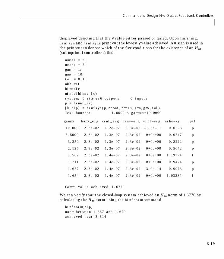
Commands to Design H∞ Output Feedback Controllers
displayed denoting that the γ value either passed or failed. Upon finishing,hinfsyn and hinfsyne print out the lowest γ value achieved. A # sign is used inthe printout to denote which of the five conditions for the existence of an H∞(sub)optimal controller failed.
nmeas = 2; ncont = 2; gmn = 1; gmx = 10; tol = 0.1; mkhimat himatic minfo(himat_ic) system: 8 states6 outputs 6 inputsp = himat_ic;[k,clp] = hinfsyn(p,ncont,nmeas,gmn,gmx,tol); Test bounds: 1.0000 < gamma<=10.0000
Gamma value achieved: 1.6770
We can verify that the closed-loop system achieved an H∞ norm of 1.6770 bycalculating the H∞ norm using the hinfnorm command.
hinfnorm(clp)norm between 1.667 and 1.679achieved near 3.814
gamma hamx_eig xinf_eig hamy–eig yinf–eig nrho–xy p/f
10.000 2.3e–02 1.2e–07 2.3e–02 –1.5e–11 0.0223 p
5.5000 2.3e–02 1.3e–07 2.3e–02 0+0e+00 0.0747 p
3.250 2.3e–02 1.3e–07 2.3e–02 0+0e+00 0.2222 p
2.125 2.3e–02 1.3e–07 2.3e–02 0+0e+00 0.5642 p
1.562 2.3e–02 1.4e–07 2.3e–02 0+0e+00 1.1977# f
1.711 2.3e–02 1.4e–07 2.3e–02 0+0e+00 0.9474 p
1.677 2.3e–02 1.4e–07 2.3e–02 –3.0e–14 0.9973 p
1.654 2.3e–02 1.4e–07 2.3e–02 0+0e+00 1.0328# f
3-19
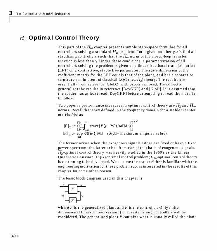
3 H∞ Control and Model Reduction
3-2
H∞ Optimal Control TheoryThis part of the H∞ chapter presents simple state-space formulae for allcontrollers solving a standard H∞ problem: For a given number γ ≥ 0, find allstabilizing controllers such that the H∞ norm of the closed-loop transferfunction is less than γ. Under these conditions, a parametrization of allcontrollers solving the problem is given as a linear fractional transformation(LFT) on a contractive, stable free parameter. The state dimension of thecoefficient matrix for the LFT equals that of the plant, and has a separationstructure reminiscent of classical LQG (i.e., H2) theory. The results areessentially from reference [GloD2] with proofs removed. This directlygeneralizes the results in reference [DoyGKF] and [GloD]. It is assumed thatthe reader has at least read [DoyGKF] before attempting to read the materialto follow.
Two popular performance measures in optimal control theory are H2 and H∞norms. Recall that they defined in the frequency domain for a stable transfermatrix P(s) as
The former arises when the exogenous signals either are fixed or have a fixedpower spectrum; the latter arises from (weighted) balls of exogenous signals.H2-optimal control theory was heavily studied in the 1960’s as the LinearQuadratic Gaussian (LQG) optimal control problem; H∞-optimal control theoryis continuing to be developed. We assume the reader either is familiar with theengineering motivation for these problems, or is interested in the results of thischapter for some other reason.
The basic block diagram used in this chapter is
where P is the generalized plant and K is the controller. Only finitedimensional linear time-invariant (LTI) systems and controllers will beconsidered. The generalized plant P contains what is usually called the plant
P 2 := 12π------ trace
∞–
∞
∫ P jω( )*P jω( )[ ]dω 1 2⁄
P ∞ := sup σ([)P jω( )] (σ :( ) = maximum singular value)ω
P
K
e
y
d
u
-
0

H∞ Optimal Control Theory
in a control problem plus all weighting functions. The signal d contains allexternal inputs, including disturbances, sensor noise, and commands, theoutput e is an error signal, y is the measured variables, and u is the controlinput. The diagram is also referred to as a linear fractional transformation(LFT) on K and P is called the coefficient matrix for the LFT. The resultingclosed loop transfer function from d to e is denoted by Ted = FL(P,K).
The main H∞ output feedback results are presented in the “H∞ OutputFeedback” section. The proofs of these results exploit the separation structureof the controller. If perfect measurements of the states (x) and the disturbances(d) are available (this is defined as the Full Information problem), then thecentral controller is simply a gain matrix F∞, obtained through finding acertain stable invariant subspace of a Hamiltonian matrix. Also, the optimaloutput estimator is an observer whose gain is obtained in a similar way from adual Hamiltonian matrix. These special cases are described in the “H∞ FullInformation and Full Control Problems” section. In the general outputfeedback case the controller can be interpreted as an optimal estimator for F∞x.Furthermore, the two Hamiltonians involved in this solution can be associatedwith full information and output estimation problems.
As mentioned, this material is taken primarily from [GloD2], which is a directgeneralization of [DoyGKF], and contains a substantial repetition of material.Roughly speaking, [GloD2] proves those results in [GloD] which were statedwithout proof, using [DoyGKF] machinery, which considered a less generalproblem. An alternative approach in relaxing some of the assumptions in[DoyGKF] is to use loop-shifting techniques as in [ZhouK], [GloD], and morecompletely in [SafLC]. We also consider some aspects of generalizations to the≤ case, primarily to indicate the problems encountered in the optimal case. Adetailed derivation of the necessity of the generalized conditions for the FullInformation problem is given. In keeping with the style of [GloD] and[DoyGKF], we don’t present a complete treatment of the ≤ case. Completederivations of the optimal output feedback case can be found in [GlovM] usingdifferent techniques.
3-21

3 H∞ Control and Model Reduction
3-2
Historical PerspectiveThis section is not intended as a review of the literature in H∞ theory, butrather an attempt to outline some of the work that led up to and most closelytouches on [DoyGKF], [GloD], and [GloD2]. Control, history For a moreextensive bibliography and review of earlier literature, the interested readermight see [Fran1] and [FranD].
Zames’ [Zame] original formulation of H∞ optimal control theory was in aninput-output setting. Most solution techniques available at that time involvedanalytic functions (Nevanlinna-Pick interpolation) or operator-theoreticmethods [Sara], [AdAK], and [BallH]. An earlier state-space solution waspresented in [Doy1], in which the steps were as follows: parametrize allinternally stabilizing controllers via Youla [YouJB]; obtain realizations of theclosed-loop transfer matrix; convert the resulting model-matching problem intothe equivalent 2 × 2-block general distance or best approximation probleminvolving mixed Hankel-Toeplitz operators; reduce to the Nehari problem(Hankel only); and solve the Nehari problem by the procedure of [Glo1]. Both[Fran1] and [FranD] give expositions of this approach, which will be referredto as the “1984” approach.
In a mathematical sense, the 1984 procedure solved the general rational H∞optimal control problem and much of the subsequent work in H∞ control theoryfocused on the 2 × 2-block problems, either in the model-matching or generaldistance forms. Unfortunately, the associated complexity of computation wassubstantial, involving several Riccati equations of increasing dimension, andformulae for the resulting controllers tended to be very complicated and havehigh state dimension. Encouragement came from [LimH] who showed, forproblems transformable to 2 × 1-block problems, that a subsequent minimalrealization of the controller has state dimension no greater than that of thegeneralized plant G. This suggested the likely existence of similarly lowdimension optimal controllers in the general 2 × 2 case.
Additional progress on the 2 × 2-block problems came from [BallC], who gave astate-space solution involving three Riccati equations. [JonJ] showed aconnection between the 2 × 1-block problem. [FoisT] developed an interestingclass of operators called skew Toeplitz to study the 2 × 2-block problem. Otherapproaches have been derived by [Hung] using an interpolation theoryapproach, [Kwak] using a polynomial approach, and [Kim] using a methodbased on conjugation.
2

H∞ Optimal Control Theory
In addition to providing controller formulae that are simple and expressed interms of plant data, the methods in the present approach are a fundamentaldeparture from the earlier work described above. In particular, the Youlaparametrization and the resulting 2 × 2-block model-matching problem of the1984 solution are avoided entirely; replaced by a pair of 2 × 1-block problemsand a separation argument. The entire development uses simple and familiartools, in the style of [Will1] relying on state feedback and observer-basedcontrol methods and more straightforward and elegant use of operator theory.Another strong influence on this work is Redheffer’s work [Red2] on linearfractional transformations.
Independent encouragement for a simpler approach to the H∞ problem camefrom papers by [KhaPZ] and [ZhoK]. They showed that for the state-feedbackH∞ problem one can choose a constant gain as a (sub)optimal controller. Inaddition, a formula for the state-feedback gain matrix was given in terms of analgebraic Riccati equation. These results are similar to those in the “H∞ FullInformation and Full Control Problems” section, though the proof techniquesare entirely different. Also, these papers established connections between H∞-optimal control, quadratic stabilization, and linear-quadratic differentialgames.
As expected, the results and techniques in [DoyGKF] and [GloD2] haveencouraged greater interest in applications of H∞ methods, in alternativedevelopments of the theory using other techniques, and in extensions to moregeneral problems. The state-space theory of H∞ can be carried much further,by generalizing time-invariant to time-varying, infinite horizon to finitehorizon, and finite dimensional to infinite dimensional. A flourish of activityhas begun on these problems and the already numerous results indicate, notsurprisingly, that many of the results generalize mutatis mutandis, to thesecases.
NotationThe notation is fairly standard. The Hardy spaces H2 and consist ofsquare-integrable functions on the imaginary axis with analytic continuationinto, respectively, the right and left half-plane. The Hardy space H∞ consists ofbounded functions with analytic continuation into the right half-plane. TheLebesgue spaces L2 = L2(–∞,∞), L2+ = L2[0,∞), and L2– = L2(–∞,0] consistrespectively of square-integrable functions on (–∞,∞), [0,∞), and (–∞,0], andL∞ consists of bounded functions on (–∞,∞). As interpreted in this chapter, L∞
H2⊥
3-23

3 H∞ Control and Model Reduction
3-2
will consist of functions of frequency, L2+ and L2– functions of time, and L2 willbe used for both.
We will make liberal use of the Hilbert space isomorphism, via the Laplacetransform and the Paley-Wiener theorem, of L2 = L2+ ⊕ L2– in the time-domainwith L2 = H2 ⊕ in the frequency-domain and of L2+ with H2 and L2– with
. In fact, we will normally not make any distinction between a time-domainsignal and its transform. Thus we may write and then treat d as if
. This style streamlines the development, as well as the notation, butwhen any possibility of confusion could arise, we will make it clear whether weare working in the time- or frequency-domain.
All matrices and vectors will be assumed to be complex. A transfer matrix interms of state-space data is denoted
For a matrix , M´ denotes its conjugate transpose,denotes its maximum singular value, ρ(M)denotes its
spectral radius (if p = r), and denotes the Moore-Penrose pseudo-inverse ofM. Im denotes image, ker denotes kernel, and . For operators,
denotes the adjoint of Γ. The prefix B denotes the open unit ball and theprefix Rc denotes complex-rational.
The orthogonal projections P+ and P– map L2 to, respectively, H2 and (orL2+ and L2–). For , the Laurent or multiplication operatorfor frequency-domain is defined by MPd = Pd. The norms on L∞ and L2in the frequency-domain were defined in the “Performance as GeneralizedDisturbance Rejection” section. Note that both norms apply to matrix orvector-valued functions. The unsubscripted norm || • ||will denote the standardEuclidean norm on vectors. We will omit all vector and matrix dimensionsthroughout, and assume that all quantities have compatible dimensions.
H2⊥
H2⊥
d L2+∈d H2∈
A BC D
:= C sI A–( ) 1– B D+
M Cp r×∈σ M( ) ρ M′M( )1 2⁄=
M†
P~ s( ) := P s–( )′Γ*
H2⊥
P L∞∈ MP : L2 L2→d L2∈
4

H∞ Optimal Control Theory
Problem StatementConsider the system described by the block diagram
Both P and K are complex-rational and proper, and K is constrained to provideinternal stability. We will denote the transfer functions from d to e as Ted ingeneral and for a linear fractional transformation feedback connection as abovewe also write Ted = FL(P,K). This section discusses the assumptions on P thatwill be used. In our application we have state models of P and K. Then internalstability will mean that the states of P and K go to zero from all initial valueswhen d = 0.
Since we will restrict our attention exclusively to proper, complex-rationalcontrollers that are stabilizable and detectable, these properties will beassumed throughout. Thus the term controller will be taken to mean acontroller that satisfies these properties. Controllers that have the additionalproperty of being internally stabilizing will be said to be admissible. Althoughwe are taking everything to be complex, in the special case where the originaldata is real (e.g., P is real-rational) then all of the results (such as K) will alsobe real.
The problem to be considered is to find all admissible K(s) such that||Ted||∞ < γ(≤ γ). The realization of the transfer matrix P is taken to be of the form
compatible with the dimensions , , ,
, and the state . The following assumptions are made:
(A1) (A,B2) is stabilizable and (C2,A) is detectable.
P
K
e
y
d
u
-
P s( )
A B1 B2
C1 D11 D12
C2 D21 D22
A BC D
= =
e t( ) Cp1∈ y t( ) C
p2∈ d t( ) Cm1∈
u t( ) Cm2∈ x t( ) Cn∈
3-25

3 H∞ Control and Model Reduction
3-2
(A2) D12 is full column rank with unitary and D21 is full row rank
with unitary.
(A3) has full column rank for all ω.
(A4) has full row rank for all ω.
Assumption (A1) is necessary for the existence of stabilizing controllers. Theassumptions in (A2) mean that the penalty on e = C1x + D12u includes anonsingular, normalized penalty on the control u, and that the exogenoussignal ω includes both plant disturbance and sensor noise, and the sensor noiseweighting is normalized and nonsingular. Relaxation of (A2) leads to singularcontrol problems.
Assumption (A3) relaxes the [DoyGKF] assumptions that (C1,A) is detectableand D´12C1 = 0, and (A4) relaxes (A,B1) stabilizable and B´1D21 = 0.Assumptions (A3) and (A4) are made for a technical reason: together with (A1)it guarantees that the two Hamiltonian matrices in the corresponding H2problem belong to dom(Ric). It is tempting to suggest that (A3) and (A4) can bedropped, but they are, in some sense, necessary for the methods in this chapterto be applicable. A further discussion of the assumptions and their possiblerelaxation will be discussed in the “Relaxing Assumptions A1–A4” section.
It will be assumed in the rest of this chapter that D22 = 0. To see how to handlethe general case for D22 ≠ 0, suppose K is a stabilizing controller for D22 set tozero, and satisfies
D12 D⊥
D21
D⊥
A jωI– B2
C1 D12
A jωI– B1
C2 D21
FL P 0 00 D22
K,–
∞γ<
6
H∞ Optimal Control Theory
then
FL(P,K(I + D22K)–1) = P11 + P12K(I + D22K – P22K)–1P21
Hence a controller K for
yields a controller for P. The µ-Tools commands hinfsyn
and hinfsyne handle the nonzero D22 case.
When D22 ≠ 0 there is a possibility of the feedback system becoming ill-poseddue to det(I +D22 = 0 (or more stringent conditions if we requirewell-posedness in the face of infinitesimal time delays [Will1]). Suchpossibilities need to be excluded.
It can be assumed, without loss of generality, that γ = 1 since this is achievedby the scalings γ–1D11, γ–1/2B1, γ–1/2C1, γ1/2B2, γ1/2C2, and γ–1K. This will bedone implicitly for many of statements of this chapter.
PreliminariesThis section reviews some mathematical preliminaries, in particular thecomputation of the various norms of a transfer matrix P. Consider the transfermatrix
(3-4)
with A stable (i.e., all eigenvalues in the left half-plane).
The norm ||P||∞ arises in a number of ways. Suppose that we apply aninput and consider the output . Then a standard result is
FL= P 0 00 D22
K,–
⋅
P0 00 D22
–
K K I D22K+( ) 1–=
K ∞( ) )
P s( ) A BC D
=
d L2∈ e L2∈
3-27

3 H∞ Control and Model Reduction
3-2
that||P||∞ is the induced norm of the multiplication operator MP, as well as theToeplitz operator .
The rest of this section involves additional characterizations of the norms interms of state-space descriptions. “The Riccati Operator” section collects somebasic material on the Riccati equation and the Riccati operator, which play anessential role in the development of both theories.
The Riccati OperatorLet A, Q, R be complex n × n matrices with Q and R Hermitian. Define the 2n× 2n Hamiltonian matrix
If we begin by assuming H has no eigenvalues on the imaginary axis, then itmust have n eigenvalues in Re s < 0 and n in Re s > 0. Consider the twon-dimensional spectral subspaces χ–(H) and χ+(H): the former is the invariantsubspace corresponding to eigenvalues in Re s < 0; the latter, to eigenvalues inRe s > 0. Finding a basis for χ–(H), stacking the basis vectors up to form amatrix, and partitioning the matrix, we get
(3-5)
where , and
(3-6)
P+MP : H2 H2→
P ∞ sup e 2 sup P+e 2 sup P+MPd 2= = =d BL2∈ d BL
2+∈ d BH2∈
H := A RQ A ′–
χ– H( ) ImX1
X2
=
X1,X2 Cn n×∈
HX1
X2
X1
X2
TX, Re λi Tx( ) 0< i∀=
8
H∞ Optimal Control Theory
If X1 is nonsingular, or equivalently, if the two subspaces
(3-7)
are complementary, we can set X := X2X1–1. Then X is uniquely determined by
H, i.e., H a X is a function, which will be denoted Ric; thus, X = Ric(H). We willtake the domain of Ric, denoted dom(Ric), to consist of Hamiltonian matricesH with two properties, namely, H has no eigenvalues on the imaginary axis andthe two subspaces in equation (3-7) are complementary. For ease of reference,these will be called the stability property and the complementary property,respectively. The following well-known results give some properties of X as wellas verifiable conditions under which H belongs to dom(Ric). See, for example,Section 7.2 in [Fran1], Theorem 12.2 in [Wonh], and [Kuc1].
Lemma 3.1. Suppose H Πdom(Ric) and X = Ric(H). Then
a X is Hermitian
b satisfies the algebraic Riccati equation
A´X + XA + XRX – Q = 0
c A + RX is stable
Lemma 3.2. Suppose H has no imaginary eigenvalues, R is either positivesemidefinite or negative semidefinite, and (A,R) is stabilizable. ThenH Πdom(Ric).
Lemma 3.3. Suppose H has the form
with (A,B) stabilizable and rank . Then H ∈ dom(Ric),
X = Ric(H) ≥ 0, and ker(X) ⊂ χ := stable unobservable subspace.
By stable unobservable subspace we mean the intersection of the stableinvariant subspace of A with the unobservable subspace of (A,C). Note that if(C,–A) is detectable, then Ric(H) ≥ 0. Also, note that ker(X) ⊂ χ ⊂ ker(C), so that
χ– H( ) I, m 0I
H A BB '–
C'C– A '–=
A jωI+ C' n ω∀=
3-29

3 H∞ Control and Model Reduction
3-3
the equation XM = C´ always has a solution for M, for example theleast-squares solution given by .
Computing the H∞ NormFor the transfer matrix P(s) in equation (3-4), with A stable, define theHamiltonian matrix
(3-8)
(3-9)
where R = I – D´D. The following lemma is essentially from [And], [Will1], and[BoyBK].
Lemma 3.4. Let , then the following conditions are equivalent:
a ||P||∞ < 1
b H has no eigenvalues on the imaginary axis
c H ∈ dom(Ric)
d H ∈ dom(Ric) and Ric(H) ≥ 0 (Ric(H) > 0 if (C,A) is observable)
Lemma 3.4 suggests the following way to compute an H∞ norm: select apositive number γ; test if ||P||∞ < γ by calculating the eigenvalues of H; increaseor decrease γ accordingly; repeat. Thus H∞ norm computation requires asearch, over either γ or ω. We should not be surprised by similar characteristicsof the H∞-optimal control problem. A somewhat analogous situation occurs formatrices with the norms and . Inprinciple, can be computed exactly with a finite number of operations, ascan the test for whether (e.g., γ2I – M*M > 0), but the value ofcannot. To compute we must use some type of iterative algorithm.
X†C ′
H := A BR 1– D 'C+ BR 1– B'
C'– I DD'–( ) 1– C A BR 1– D 'C+( ) '–
A 0C ′C– A′–
BC′D–
R 1–D′C B′+=
σ D( ) 1<
M 22 trace M*M( )= M ∞ σ M[ ]=
M 22
σ M( ) γ< σ M( )σ M( )
0

H∞ Full Information and Full Control Problems
H∞ Full Information and Full Control ProblemsIn this section we discuss four problems from which the output feedbacksolutions will be constructed via a separation argument. These specialproblems are central to the whole approach taken in this chapter, and as weshall see, they are also important in their own right. All pertain to the standardblock diagram,
but with different structures for P. The problems are labeled
FC and OE are natural duals of FI and DF, respectively. The DF solution canbe easily obtained from the FI solution, as shown in the “DisturbanceFeedforward and Output Estimation” section. The output feedback solutionswill be constructed out of the FI and OE results. A dual derivation could usethe FC and DF results.
The FI and FC problems are not, strictly speaking, special cases of the outputfeedback problem, as they do not satisfy all of the assumptions. Each of the fourproblems inherit certain of the assumptions A1–A4 from the “ProblemStatement” section as appropriate. The terminology and assumptions will bediscussed in the subsections for each problem. In each of the four cases, theresults are necessary and sufficient conditions for the existence of a controllersuch that ||Ted||∞ < γ and the family of all controllers such that ||Ted||∞ < γ. In allcases, K must be admissible.
FI Full information
FC Full control
DF Disturbance feedforward (to be considered in the “DisturbanceFeedforward and Output Estimation” section)
OE Output estimation (to be considered in the “DisturbanceFeedforward and Output Estimation” section)
P
K
e
y
d
u
-
3-31

3 H∞ Control and Model Reduction
3-3
The H∞ solution involves two Hamiltonian matrices, H∞ and J∞, which aredefined as follows:
(3-10)
(3-11)
If H∞ ∈ dom(Ric) then let X1, X2 be any matrices such that
(3-12)
Similarly if J∞ ∈ dom(Ric) then let Y1, Y2 be any matrices such that
(3-13)
Also define
(3-14)
Finally define the state feedback and output injection matrices as
R := D ′1•D1•γ2Im1
0
0 0, where D1• := D11 D12–
R := D•1D ′•1γ2
Ip10
0 0, where D•1 :=
D11
D21
–
H∞ :=A 0
C ′– 1C1 A ′B
C′– 1D1•R 1–
D′1•C1 B′–
J∞ :=A ′ 0
B– 1B′1 A–
C′B– 1D ′•1
R1–
D•1B′1 C–
H∞X1
X2
X1
X2
TX, X1′ X2 X2′ X1,= Re λi TX( ) ð 0 i∀=
J∞Y1
Y2
Y1
Y2
TY, Y1′ Y2 Y2′ Y1= Re λi TY( ) ð 0 i∀=
X∞ := X2X11– , Y∞ := Y2Y1
1–
2

H∞ Full Information and Full Control Problems
(3-15)
(3-16)
Problem FI: Full InformationIn the full information (FI) special problem P has the following form:
(3-17)
It is seen that the controller is provided with full information since
. In some cases, a suboptimal controller may exist which uses just
the state feedback x, but this will not always be possible. While the statefeedback problem is more traditional, we believe that the Full Informationproblem is more fundamental and more natural than the state feedbackproblem, once you get outside the pure H2 setting.
The assumptions relevant to the FI problem, which are inherited from theoutput feedback problem, are
(A1) (A,B2) is stabilizable.
(A2) D12 is full column rank with unitary.
(A3) has full column rank for all ω.
F :=F1
F2
:= R–1– D′1•C1 B′+ X∞[ ]
L := L1 L2 := – B1D′•1 Y∞+ C′[ ]R
1–
P s( )
A B1 B2
C1 D11 D12
I0
0I
00
=
y xd
=
D12 D⊥
A jωI– B2
C1 D12
3-33

3 H∞ Control and Model Reduction
3-3
The results for the Full Information case are as follows:
Theorem 3.5. Suppose P is given by (3-17) and satisfies A1–A3. Then,
a ∃K such that ||Ted||∞ < 1 H∞ ∈ dom(Ric), Ric(H∞) ≥ 0
b All admissible K(s) such that ||Ted||∞ < 1 are given by
for Q ∈ RcH∞, ||Q||∞ < 1.
Problem FC: Full ControlThe full control (FC) problem has P given by,
(3-18)
and is the dual of the Full Information case: the P for the FC problem has thesame form as the transpose of P for the FI problem. The term Full Control isused because the controller has full access to both the state through outputinjection and to the output e. The only restriction on the controller is that itmust work with the measurement y. The assumptions that the FC probleminherits from the output feedback problem are just the dual of those in the FIproblem:
(A1) (C2,A) is detectable.
(A2) D21 is full row rank with unitary.
(A4) has full row rank for all ω.
K s( ) Q s( )– IT1 0
T2 I
F1 I–
F2 0=
P s( )
A B1 I 0
C1 D11 0 I
C2 D21 0 0
=
D21
D⊥
A jωI– B1
C2 D21
4

H∞ Full Information and Full Control Problems
Necessary and sufficient conditions for the FC case are given in the followingcorollary. The family of all controllers can be obtained from the dual ofTheorem 3.5 but these controllers will not be required in the sequel and arehence omitted.
Corollary 3.6. Suppose P is given by (3-18) and satisfies A1, A2 and A4. Then,
∃K such that ||Ted||∞ < 1 J∞ ∈ dom(Ric), Ric(J∞) ≥ 0
3-35

3 H∞ Control and Model Reduction
3-3
H∞ Output FeedbackThe solution to the Full Information problem of the “H∞ Full Information andFull Control Problems” section is used in this section to solve the outputfeedback problem. First in Theorem 3.8 a so-called disturbance feedforwardproblem is solved. In this problem one component of the disturbance, d2, can beestimated exactly from y using an observer, and the other component of thedisturbance, d1, does not affect the state or the output. The conditions for theexistence of a controller satisfying a closed-loop H∞-norm constraint is thenidentical to the FI case.
The solution to the general output feedback problem can then be derived fromthe transpose of Theorem 3.7 (Corollary 3.9) by a suitable change of variableswhich is based on X∞ and the completion of the squares argument (see[GloD2]).
The main result is now stated in terms of the matrices defined in the “H∞ FullInformation and Full Control Problems” section involving the solutions of theX∞ and Y∞ Riccati equations together with the state feedback and outputinjection matrices F and L. Assume that unitary changes of coordinates on ωand z have been carried out to give the following partitions of D, F1 and L1.
(3-19)
Theorem 3.7. Suppose P satisfies the assumptions A1–A4 of the “ProblemStatement” section.
a There exists an admissible controller K(s) such that||FL(P,K)||∞ < γ (i.e., ||Ted||∞ < γ) if and only if
i γ > max
ii H∞ ∈ dom(Ric) with X∞ = Ric(H∞) ≥ 0
iii J∞ ∈ dom(Ric) with Y∞ = Ric(J∞) ≥ 0
iv ρ(X∞Y∞) < γ2.
F ′L′ D
F′11 F ′12 F′2L ′11 D1111 D1112 0
L ′12 D1121 D1122 I
L′2 0 I 0
=
σ D1111 D1112,[ ],σ D ′1111 D ′1121,[ ]( )
6

H∞ Output Feedback
b Given that the conditions of part (a) are satisfied, then all rationalinternally stabilizing controllers K(s) satisfying ||FL(P,K)||∞ < γ are givenby
K = FL(Ka,Φ) for arbitrary Φ ∈ RcH∞ such that ||Φ||∞
< γ
where
and are any matrices (e.g., Cholesky factors)satisfying
and
where
(Note that if D11 = 0 then the formulae are considerably simplified.)
Ka
Aˆ
B1ˆ
B2ˆ
C1ˆ
D11ˆ
D12ˆ
C2ˆ
D21ˆ
0
=
D11ˆ
D– 1121D ′1111 γ2I D1111D ′1111–( )1–
D1112 D1122,–=
D12ˆ
Cm2 m2×
∈ D21ˆ
Cp2 p2×
∈
D12ˆ
D12ˆ
I D1121– γ2I D ′1111D1111–( )1–
D1121,=
D21ˆ
D21ˆ
I D ′1112– γ2I D1111D′1111–( )1–
D1112,=
B2ˆ
Z∞1– B2 L12+( ) D12
ˆ,=
C2ˆ
D– 21ˆ
C2 F12+( ),=
B1ˆ
Z– ∞1– L2 B2
ˆ+ D
ˆ12
1–D11,=
C1ˆ
F2 Dˆ
11+ Dˆ
211–
Cˆ
2,=
Aˆ
A BF+ Bˆ
1+ Dˆ
211–
Cˆ
2,=
Z∞ I γ 2– Y∞X∞–( )= .
3-37
3 H∞ Control and Model Reduction
3-3
The proof of this main result is via some special problems that are simplerspecial cases of the general problem and can be derived from the FI and FCproblems. A separation type argument can then give the solution to the generalproblem from these special problems. It can be assumed, without loss ofgenerality, that γ = 1 since this is achieved by the scalings γ–1D11, γ–1/2B1,γ–1/2C1, γ1/2B2, γ1/2C2, γ-1X∞, γ-1Y∞ and γ–1K. All the proofs will be given for thecase γ = 1.
Disturbance Feedforward and Output EstimationIn the Disturbance Feedforward problem one component of the disturbance, d1,does not affect the state or the output. The other component of the disturbance,d2 (and hence the state x), can be estimated exactly from y using an observer.The conditions for the existence of a controller satisfying a closed-loopH∞-norm constraint is then identical to the Full Information case.
Theorem 3.8. (Disturbance Feedforward)
Theorem 3.7 is true under the additional assumptions that
(3-20)
In this case,
The transpose of Theorem 3.8 can now be stated to obtain another special caseof Theorem 3.7.
Corollary 3.9. (Output Estimation)
Theorem 3.7 is true under the additional assumptions that
In this case
B1D ′˜⊥ 0, A B1D ′21C2 is stable.–=
Y∞ 0, Z I, L 0 B1D ′21–===
D′⊥C1 0, A B2D ′12C1 is stable.–=
X∞ 0, Z I, F0
D ′12C1–===
8

H∞ Output Feedback
Converting Output Feedback to Output EstimationThe output feedback case when the disturbance, d, cannot be estimated fromthe output is reduced to the case of Corollary 3.9 by the change of variables
where
We will perform the change of variables with v replacing e and r replacing d.Hence
and the transfer matrix from to is
(3-21)
Similarly substituting v for u in the equation for P gives that the transfer
function from to is H as defined by
(3-22)
e 22 d 2
2– v 2
2 r 22
–=
v u T2d T2, I Fx–+=
r T1 2( ) d F1x–( )=
x· A B1F1+( )x B1T11– r B2u+ +=
v u T2T11– r F2x–+=
y C2x D21T11– r D21F1x+ +=
ru
vy
Pvyru s( ) :=
A B1F1+ B1T11– B2
F– 2 T2T11– I
C2 D21F1+ D21T11– 0
dv
er
H
Q
e
r
d
v
-
H =
264
AF B1 B2T2 B2
C1F1 D?D0
?D11 D12
T1F1 T1 0
375
3-39

3 H∞ Control and Model Reduction
3-4
It can be shown that H~H = I (since ) and that AF isstable.
We can show with a little algebra the equivalence of the first two of thefollowing block diagrams, with Tvr = FL(Pvyru,K) given by the third one.
Lemma 3.10. Let P satisfy A1–A4, and assume that X∞ exists and X∞ ≥ 0. Thenthe following are equivalent:
a K internally stabilizes P and ||FL(P,K)||∞ < 1,
b K internally stabilizes Pvyru and ||FL(Pvyru,K)||∞ < 1
c K internally stabilizes Ptmp and ||FL(Ptmp,K)||∞ < 1,
where Pvyru is given by (3-21) and
The importance of the above constructions for Pvyru and Ptmp is that theysatisfy the assumptions for the output estimation problem (Corollary 3.9) sinceA + BF is stable.
Relaxing Assumptions A1–A4In this section we indicate how the results of the “H∞ Output Feedback” sectioncan be extended to more general cases by the relaxation of assumptions A1–A4.The optimal case is not considered, but the interested reader may refer to[GloD2].
e 22 d 2
2– v 2
2 r 22
–=
P
K
e
y
d
u
-
H
Tvr
e
r
d
v
-
Pvyru
K
v
y
r
u
-
Ptmp :=
A B1F1+ B1 B2
D12F– 2 D11 D12
C2 D21F1+ D21 0
.
0
H∞ Output Feedback
Relaxing A3 and A4 Suppose that,
which violates both A3 and A4 and corresponds to the robust stabilization of anintegrator. If the controller u = –εx, for ε > 0 is used then
Hence the norm can be made arbitrarily small as ε → 0, but ε = 0 is notadmissible since it is not stabilizing. This may be thought of as a case wherethe H∞-optimum is not achieved on the set of admissible controllers. Of course,for this system, H∞ optimal control is a silly problem, although the suboptimalcase is not obviously so.
If you simply drop the requirement that controllers be admissible and removeassumptions A3 and A4, then the formulae in this chapter will yield u = 0 forboth the optimal controller and the suboptimal controller with Φ = 0. Thisillustrates that assumptions A3 and A4 are necessary for the techniques in thischapter to be directly applicable. An alternative is to develop a theory thatmaintains the same notion of admissibility, but relaxes A3 and A4. The easiestway to do this would be to pursue the suboptimal case introducing εperturbations so that A3 and A4 are satisfied.
Relaxing A1If assumption A1 is violated, then it is obvious that no admissible controllersexist. Suppose A1 is relaxed to allow unstabilizable and/or undetectable modeson the jω axis, and internal stability is also relaxed to also allow closed-loop jωaxis poles, but A2–A4 is still satisfied. It can be easily shown that under theseconditions the closed-loop H∞ norm cannot be made finite, and in particular,that the unstabilizable and/or undetectable modes on the jω axis must show upas poles in the closed-loop system.
P0 0 10 0 11 1 0
=
Tedεs–
s ε+-----------, with Ted ∞ ε==
3-41

3 H∞ Control and Model Reduction
3-4
Violating A1 and Either or Both of A3 and A4Sensible control problems can be posed that violate A1 and either or both of A3and A4. For example, cases when A has modes at s = 0, which are unstabilizablethrough B2 and/or undetectable through C2, arise when an integrator isincluded in a weight on a disturbance input or an error term. In these cases,either A3 or A4 is also violated, or the closed-loop H∞ norm cannot be madefinite. In many applications such problems can be reformulated so that theintegrator occurs inside the loop (essentially using the internal modelprinciple), and is hence detectable and stabilizable.
An alternative approach to such problems, which could potentially avoid theproblem reformulation, would be to pursue the techniques in [GloD2], but relaxinternal stability to the requirement that all closed-loop modes be in the closedleft half plane. Clearly, to have finite H∞ norm these closed-loop modes couldnot appear as poles in Ted. The formulae given in this chapter will often yieldcontrollers compatible with these assumptions. You would then have to decidewhether closed-loop poles on the imaginary axis were due to weights and henceacceptable or due to the problem being poorly posed as in the above example.
A third alternative is to again introduce ε perturbations so that A1, A3 and A4are satisfied. Roughly speaking, this would produce sensible answers forsensible problems, but the behavior as ε → 0 could be problematic.
Relaxing A2In the case that either D12 is not full column rank or D21 is not full row rank,then improper controllers can give bounded H∞-norm for Ted, although will notbe admissible as defined in the “Problem Statement” section. Such singularfiltering and control problems have been well-studied in H2 theory and manyof the same techniques go over to the H∞ -case (e.g., [Will2], [WilKS] and[HauS]). In particular the structure algorithm of [Silv] could be used to makethe terms D12 and D21 full rank by the introduction of suitable differentiatorsin the controller.
2
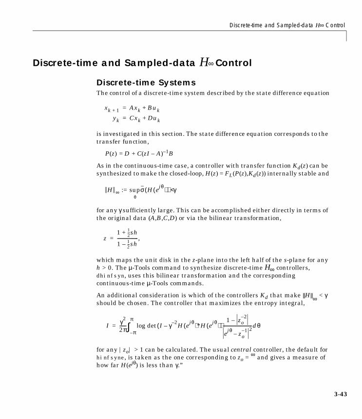
Discrete-time and Sampled-data H∞ Control
Discrete-time and Sampled-data H∞ Control
Discrete-time SystemsThe control of a discrete-time system described by the state difference equation
is investigated in this section. The state difference equation corresponds to thetransfer function,
P(z) = D + C(zI – A)–1B
As in the continuous-time case, a controller with transfer function Kd(z) can besynthesized to make the closed-loop, H(z) = FL(P(z),Kd(z)) internally stable and
for any γ sufficiently large. This can be accomplished either directly in terms ofthe original data (A,B,C,D) or via the bilinear transformation,
which maps the unit disk in the z-plane into the left half of the s-plane for anyh > 0. The µ-Tools command to synthesize discrete-time H∞ controllers,dhinfsyn, uses this bilinear transformation and the correspondingcontinuous-time µ-Tools commands.
An additional consideration is which of the controllers Kd that make ||H||∞ < γ should be chosen. The controller that maximizes the entropy integral,
for any |zo| > 1 can be calculated. The usual central controller, the default forhinfsyne, is taken as the one corresponding to zo = ∞ and gives a measure ofhow far H(ejθ) is less than γ.”
xk 1+ Axk Buk+=
yk Cxk Duk+=
H ∞ := supσ H ejθ( )( ) γ<θ
z1 1
2---sh+
1 12---sh–
-------------------,=
I γ2
2π------ log det
π–
π
∫ I γ 2–– H ejθ( )*H ejθ( )( )
1 zo2–
–
ejθ zo1–
–2
---------------------------dθ=
3-43

3 H∞ Control and Model Reduction
3-4
Sampled-data SystemsContinuous-time systems where measurements are sampled and then thecontrol signal calculated by a discrete-time controller followed by a hold aretermed sampled-data systems. Two possible H∞-type approaches to sampleddata control law design are available in µ-Tools software.
Consider the system in Figure 3-7, where P is the continuous-time generalizedplant, d is a continuous-time disturbance signal, e is a continuous-time errorsignal, y is the measurement to be sampled by the sampler S, with samplingperiod h, and u is the control signal, which is the output of the hold device, H,and is constant between sampling points.
Figure 3-7 Sampled Data System Block Diagram
If it is assumed that the input d is in fact piecewise constant (synchronizedwith u), and that only the sampled values of e are of interest, then there is adiscrete-time equivalent system for P that relates the discrete-time inputs andoutputs. The controller can then be designed using discrete-time H∞techniques.
This approach has two potential problems; one is that the intersample behaviorof the outputs is ignored and the other is that the inputs are assumed piecewiseconstant. An alternative approach is to require that the induced norm betweenthe inputs d and outputs e be less than γ,
This will handle both the above difficulties and has been studied in detail byBamieh and Pearson [BamP] along with a number of other researchers
--
- HS Kd
Puy
e d
supe L2
d L2
------------- γ<w
4

Discrete-time and Sampled-data H∞ Control
[HarK,KabH,Toi,Yam]. It turns out that if γ is achievable then it can beachieved by a linear time-invariant controller of the same degree as thegeneralized plant, P. The computations for this controller involve calculatingan equivalent discrete-time system and then using discrete-time H∞ methods.
Discrete-time and Sampled-data ExampleThe following example is meant to illustrate the discrete-time andsampled-data norms involved rather than be representative of controllerdesign. Consider the system in Figure 3-8 where,
Figure 3-8 Sampled-data System Block Diagram for Simple Example
This gives the generalized plant,
F1 s( ) 11 τ1s+( )
-----------------------=
F2 s( )ωo
2
s2 2cωos ωo2
+ +( )----------------------------------------------=
F3 s( ) 11 τ3s+( )
-----------------------=
f
6
?F1 F2
F3
SH Kd
u y
e d
PP11 s( ) P12 s( )
P21 s( ) P22 s( ),
F1F2 F1
F3 0,==
3-45

3 H∞ Control and Model Reduction
3-4
and the closed-loop is trying to match the output of F2 by the controller outputbased on the sampled input to F2 filtered by F3. P can be defined as follows:
h = 0.1;tau1 = 0.001;om_o = 2*pi; c = 0.05;tau3 = 0.01;F1 = nd2sys(1,[tau1 1]);F2 = nd2sys(1,[omo_o(-2) 2*c/omo_o 1]);F3 = nd2sys(1,[tau3 1]);p_ic = abv(mmult(F1,sbs(F2,1)),sbs(F3,0));ncon = 1; nmeas = 1;minfo(p_ic) system: 4 states 2 outputs 2 inputs
The zero controller will result in a purely continuous-time system with inducednorm given by ||P11(s)||∞:
hinfnorm(sel(p_ic,1,1)) norm between 10.01 and 10.02 achieved near 6.267
Now let us design a controller for this sampled-data system using thecorresponding sample and hold discrete-time system. The variable delaycorresponds to the number of sample delays in the controller.
gmin =.001; delay = 0; gmax = 1; tol = 0.001; tol2 = 0.001; p_ic_sh = samhld(p_ic,h); if delay>0,p_ic_sh=mmult(daug(1,nd2sys(1,eye(1,delay+1))),p_ic_sh;end[k_d,g_d,gfin_d] = ...dhfsyn(p_ic_sh,nmeas,ncon,gmin,gmax,tol,h,inf,–1,–2);
6
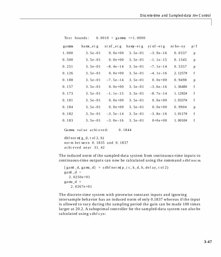
Discrete-time and Sampled-data H∞ Control
Test bounds: 0.0010 < gamma <=1.0000
Gamma value achieved: 0.1844
dhfnorm(g_d,tol2,h)norm between 0.1835 and 0.1837achieved near 31.42
The induced norm of the sampled-data system from continuous-time inputs tocontinuous-time outputs can now be calculated using the command sdhfnorm.
[gaml_d,gamu_d] = sdhfnorm(p_ic,k_d,h,delay,tol2)gaml_d =
2.0250e+01gamu_d =
2.0267e+01
The discrete-time system with piecewise constant inputs and ignoringintersample behavior has an induced norm of only 0.1837 whereas if the inputis allowed to vary during the sampling period the gain can be made 100 timeslarger at 20.2. A suboptimal controller for the sampled-data system can also becalculated using sdhfsyn:
gamma hamx_eig xinf_eig hamy–eig yinf–eig nrho–xy p/f
1.000 3.5e–01 0.0e+00 3.5e–01 –3.9e–16 0.0337 p
0.500 3.5e–01 0.0e+00 3.5e–01 –1.1e–15 0.1345 p
0.251 3.5e–01 –8.4e–14 3.5e–01 –7.1e–14 0.5357 p
0.126 3.5e–01 0.0e+00 3.5e–01 –4.1e–16 2.1257# f
0.188 3.5e–01 –7.5e–14 3.5e–01 0.0e+00 0.9498 p
0.157 3.5e–01 0.0e+00 3.5e–01 –3.6e–16 1.3648# f
0.173 3.5e–01 –1.1e–15 3.5e–01 –8.7e–14 1.1292# f
0.181 3.5e–01 0.0e+00 3.5e–01 0.0e+00 1.0337# f
0.184 3.5e–01 0.0e+00 3.5e–01 0.0e+00 0.9904 p
0.182 3.5e–01 –3.5e–14 3.5e–01 –3.8e–16 1.0117# f
0.183 3.5e–01 –3.0e–16 3.5e–01 0+0e+00 1.0010# f
3-47

3 H∞ Control and Model Reduction
3-4
[k_sd,gfin_sd]=sdhfsyn(p_ic,1,1,gmin,gamu_d,tol,h,delay,-2);Test bounds: 0.0010 < gamma <=20.2670
Gamma value achieved: 8.9601
and the norm checked by:
[gaml_sd,gamu_sd] = sdhfnorm(p_ic,k_sd,h,delay,tol2)gaml_sd =
8.9445e+00gamu_sd =
9.0028e+00
The initial design gave very low estimates of the possible gain in the system.The latter design indicates that no controller can give a low gain with thissampled-data problem. The main difficulty with this particular problem is that
gamma hamx_eig xinf_eig hamy–eig yinf–eig nrho_xy p/f
20.267 3.5e–01 –1.6e–30 3.le–01 1.0e–09 0.0016 p
10.134 3.4e–01 1.3e–31 1.6e–01 1 0e–09 0.0087 p
5.067 3.3e–01 –2.7e–20 8.3e–17# ******* ******* f
7.601 3.4e–01 2.3e–20 3.8e–15# ******* ******* f
8.867 3.4e–01 3.7e–21 1.2e–14# ******* ******* f
9.501 3.4e–01 l.le–l9 1.2e–01 1.0e–09 0.0109 p
9.184 3.4e–01 –5.3e–20 7.6e–02 1.0e–09 0.0128 p
9.026 3.4e–01 5.5e–21 4.2e–02 1.0e–09 0.0145 p
8.947 3.4e–01 1.3e–31 9.4e–14# ******* ******* f
8.986 3.4e–01 –7.7e–20 2.7e–02 1.0e–09 0.0153 p
8.966 3.4e–01 –1.5e–31 1.3e–02 1 0e–09 0.0160 p
8.956 3.4e–01 4.1e–20 3.9e–13# ******* ******* f
8.961 3.4e–01 4.9e-20 6.6e-03 1 0e–09 0.0163 p
8.959 3.4e–01 7.6e-20 8.7e-14# ******* ******* f
8.960 3.4e–01 3.5e-03 3.2e-03 1 0e–09 0.0165 p
8.960 3.4e–01 -2.3e-20 9.0e-14# ******* ******* f
8

Discrete-time and Sampled-data H∞ Control
the filter F3(s) has too high a bandwidth and this gives a high potential gain forF3 followed by the sampler. In contrast to the continuous-time case, thecalculation of a worst-case disturbance in the sampled-data case is notstraightforward. However the time domain simulation of the system is nowperformed to illustrate the reason for its high gain.
tfinal = 10; t1 = (0:h/100:tfinal)'; [nr,nc] = size(t1); w1 = zeros(nr,nc); for i = 1:length(t1)/200,w1(100*i–20:100*i) = ...cos(i*pi/5–pi/6)*exp(h*(–20:1:0)/(100*tau3))';...endw = vpck(w1,t1); [z_d,y_d,u_d] = sdtrsp(p_ic,k-d,w,h,tfinal,h/100); vplot(z_d,'-',y_d,'.') gain_d = norm(vunpck(z-d),2)/vnorm(vunpck(w),2)gain_d =
1.2924e+01
The time responses are given in Figure 3-9 and the high gain achieved by thedisturbance being large just before the sampling instant and zero elsewhere,hence having a relatively low total energy.
3-49

3 H∞ Control and Model Reduction
3-5
Figure 3-9 Discrete-time Controller Time Response
The suboptimal sampled-data controller can be simulated with the same inputas follows:
[z_sd,y_sd,u_sd] = sdtrsp(p_ic,k_sd,w,h,tfinal,h/100); vplot(z_sd,'-',y_sd,'.') gain_sd = norm(vunpck(z_sd),2)/vnorm(vunpck(w),2)gain_sd =
6.3332e–01
The time responses are given in Figure 3-10. The gain in this instance is muchlower for this particular input. However other inputs can give a gain of close tonine.
The same example can be repeated for different values of the sampling period,h, and the controller delay, and for variations in the time constants. The twocontrollers often give very similar results, however, the discrete-time resultsobtained from samhld and dhfsyn can give optimistic gain estimates whencompared with those obtained by sdhfsyn.
0 1 2 3 4 5 6 7 8 9 10-4
-3
-2
-1
0
1
2
3
4
0

Discrete-time and Sampled-data H∞ Control
Figure 3-10 Sampled-data Controller Time Response
0 1 2 3 4 5 6 7 8 9 10-0.6
-0.4
-0.2
0
0.2
0.4
0.6
3-51

3 H∞ Control and Model Reduction
3-5
Loop Shaping Using H∞ SynthesisA particularly straightforward method of designing controllers is to use acombination of loop shaping and robust stabilization as proposed in McFarlaneand Glover [McFG1, McFG2]. Given a system with transfer function G(s) theproblem set up is given in Figure 3-11.
Figure 3-11 H∞ Loop Shaping Standard Block Diagram
The first step is to design a pre-compensator W1(s), so that the gain ofW2(s)G(s)W1(s) is sufficiently high at frequencies where good disturbanceattenuation is required and is sufficiently low at frequencies where good robuststability is required. The second step is to design a feedback controller, K∞, sothat
which will also give robust stability of the perturbed weighted plant
where NM–1 = W2GW1 is a normalized coprime factorization satisfyingN(jω)*N(jω) + M(jω)*M(jω) = I. This stability margin is always less than 1 andgives a good indication of robust stability to a wide class unstructuredperturbations. Stability margin values of ε > 0.2 – 0.3 are generally considered
ii ?
6
--
?
K1
W1GW2
reference (r)
e2 = y
e1 = ud2d1
1b W2GW1 K∞,( )---------------------------------------- :=
IK∞
I W2GW1 K∞,–( ) 1– W2GW1 I,[ ]∞
ð1ε---
N ∆1+( ) M ∆2+( ) 1– for∆1
∆2 ∞
b W2GW1 K∞,( )<
2

Loop Shaping Using H∞ Synthesis
satisfactory. The closed-loop H∞-norm performance objective has the standardsignal gain interpretation. Finally it can be shown that the controller, K∞, doesnot substantially affect the loop shape in frequencies where the gain of W2GW1is either high or low, and will guarantee satisfactory stability margins in thefrequency region of gain crossover. In the regulator setup, the final controllerto be implemented is W1K∞W2 in the feedback configuration shown in Figure3-12.
Figure 3-12 H∞ Loop Shaping Controller Implementation
Closely related to the above problem is the approach to uncertainty using thegap family of metrics. These metrics, δ(G0,G1), give a numerical value between0 and 1 for the distance between any two linear systems G0(s) and G1(s) thathave the same number of inputs and outputs. The gap metric was introducedinto the control literature by Zames and El-Sakkary [ZamE] and exploited byGeorgiou and Smith [GeoSm]. It can be computed using an H∞ optimizationproblem [Geo]. An interesting new metric, ν-gap (nugap), was derived byVinnicombe [Vin] and has a frequency response interpretation. For both ofthese metrics, the following robust performance result holds [QiuD, Vin].
(3-23)
where
The nugap is always less than or equal to the gap, so its predictions using theabove robustness results are tighter. To make use of the gap metrics in robustdesign, weighting functions need to be introduced. In the above robustness
- W2-
-
reference (r)
K1- W1
G
arcsinb G1 K1,( ) arcsinb G0 K0,( )≥ arcsinδν G0 G1,( ) arcsinδν K0 K1,( )––
b G K,( ) IK
I GK–( ) 1–G I
∞
1–
.=
3-53

3 H∞ Control and Model Reduction
3-5
result G needs to be replaced by W2GW1 and K by (similarly for G0,
G1, K0, and K1). This makes the weighting functions compatible with the
weighting structure in the loop shaping H∞ synthesis.
The interpretation of this result is that if a nominal plant G0 is stabilized bycontroller K0, with stability margin b(G0,K0), then the stability margin whenG0 is perturbed to G1 and K0 is perturbed to K1 is degraded by no more thanthe above formula. Note that 1/b(G,K) is also the signal gain from disturbanceson the plant input and output to the input and output of the controller. Modelreduction of the system model and controller can be performed by usingbalanced truncations or Hankel norm approximation of normalized coprimefactor representation.
If a reference signal (r) is available, then there is a variety of methods toincorporate the tracking error into the objective. One effective procedure is tochoose a coprime factorization of K∞ = UV–1 and let M = V–1(r +Uy) where r isthe reference and y the measurement. U and V can be obtained from aparticular observer form of K∞ in such a way that with closed-loop y = Nr andG = NM–1 is a normalized coprime factorization [Vin]. The DC. gain of thiscontroller could then be adjusted to give zero steady state tracking error.Alternatively, this nominal command response could be diagonalized and afurther command compensation performed. These ideas are applied to the“HIMAT Robust Performance Design Example” section in Chapter 7.
W11– KW2
1–
4

Model Reduction
Model ReductionIt is often desirable to approximate a state-space representation of a systemwith a lower order state-space representation. This procedure is referred to asa model reduction. The µ-Analysis and Synthesis Toolbox (µ-Tools) providesseveral commands to aid in reducing the order of a system. These are discussedin this section along with an example to illustrate their use.
Given a SYSTEM matrix [A B; C D], the simplest method of model reductionis to truncate a part of the SYSTEM A matrix and remove the correspondingcolumns and rows of the B and C matrices. The command strunc performs thisfunction. You should be careful to order the modes of the A matrix and truncatemodes that do not significantly affect the system response. The commandstrans is useful in this context as it transforms the A matrix into blockdiagonal form with 1 × 1 or 2 × 2 blocks corresponding to the respectively realand complex poles in order of increasing magnitude. This is often done prior totruncating high frequency modes.
Truncating high frequency modes will also affect the low frequency response ofthe various transfer functions. The command sresid can be used to residualizethe truncated modes and compensate for the zero frequency contribution ofeach truncated mode with an additional D matrix term in the resulting reducedorder SYSTEM matrix.
More advanced model reduction techniques for stable systems can beperformed with the µ-Tools commands sysbal and hankmr. sysbal performs abalanced realization on the input SYSTEM matrix, which entails balancing theobservability and controllability Grammians (for a more detailed discussionsee [Enn], [Glo1] and [Moo]). In its simplest form, this command will removeall unobservable and/or uncontrollable modes. sysbal also returns a vector ofthe Hankel singular values of the system, which can be used to furthertruncate the modes of the SYSTEM.
The following example illustrates how sysbal can be used to removeunobservable and uncontrollable modes. Two systems, P and C, are created andthen interconnected with unity gain negative feedback. The closed-loop system,clp, is given by
clpPC
1 PC+----------------=
3-55
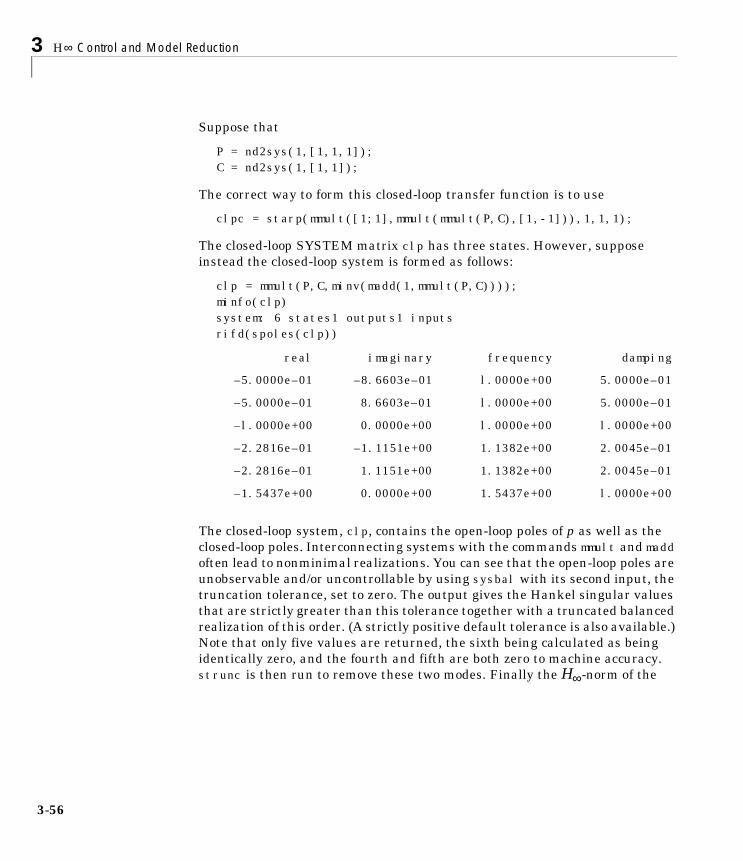
3 H∞ Control and Model Reduction
3-5
Suppose that
P = nd2sys(1,[1,1,1]); C = nd2sys(1,[1,1]);
The correct way to form this closed-loop transfer function is to use
clpc = starp(mmult([1;1],mmult(mmult(P,C),[1,-1])),1,1,1);
The closed-loop SYSTEM matrix clp has three states. However, supposeinstead the closed-loop system is formed as follows:
clp = mmult(P,C,minv(madd(1,mmult(P,C)))); minfo(clp) system: 6 states1 outputs1 inputsrifd(spoles(clp))
The closed-loop system, clp, contains the open-loop poles of p as well as theclosed-loop poles. Interconnecting systems with the commands mmult and maddoften lead to nonminimal realizations. You can see that the open-loop poles areunobservable and/or uncontrollable by using sysbal with its second input, thetruncation tolerance, set to zero. The output gives the Hankel singular valuesthat are strictly greater than this tolerance together with a truncated balancedrealization of this order. (A strictly positive default tolerance is also available.)Note that only five values are returned, the sixth being calculated as beingidentically zero, and the fourth and fifth are both zero to machine accuracy.strunc is then run to remove these two modes. Finally the H∞-norm of the
real imaginary frequency damping
–5.0000e–01 –8.6603e–01 l.0000e+00 5.0000e–01
–5.0000e–01 8.6603e–01 l.0000e+00 5.0000e–01
–l.0000e+00 0.0000e+00 l.0000e+00 l.0000e+00
–2.2816e–01 –1.1151e+00 1.1382e+00 2.0045e–01
–2.2816e–01 1.1151e+00 1.1382e+00 2.0045e–01
–1.5437e+00 0.0000e+00 1.5437e+00 l.0000e+00
6
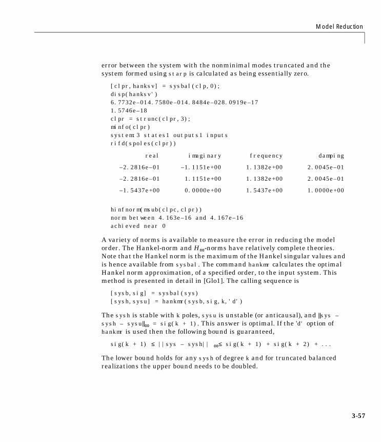
Model Reduction
error between the system with the nonminimal modes truncated and thesystem formed using starp is calculated as being essentially zero.
[clpr,hanksv] = sysbal(clp,0); disp(hanksv') 6.7732e–014.7580e–014.8484e–028.0919e–171.5746e–18clpr = strunc(clpr,3); minfo(clpr)system:3 states1 outputs1 inputsrifd(spoles(clpr))
hinfnorm(msub(clpc,clpr))norm between 4.163e–16 and 4.167e–16achieved near 0
A variety of norms is available to measure the error in reducing the modelorder. The Hankel-norm and H∞-norms have relatively complete theories.Note that the Hankel norm is the maximum of the Hankel singular values andis hence available from sysbal. The command hankmr calculates the optimalHankel norm approximation, of a specified order, to the input system. Thismethod is presented in detail in [Glo1]. The calling sequence is
[sysb,sig] = sysbal(sys) [sysh,sysu] = hankmr(sysb,sig,k,'d')
The sysh is stable with k poles, sysu is unstable (or anticausal), and ||sys – sysh – sysu||∞ = sig(k + 1). This answer is optimal. If the 'd' option ofhankmr is used then the following bound is guaranteed,
sig(k + 1) ≤ ||sys – sysh|| ∞≤ sig(k + 1) + sig(k + 2) + ...
The lower bound holds for any sysh of degree k and for truncated balancedrealizations the upper bound needs to be doubled.
real imaginary frequency damping
–2.2816e–01 –1.1151e+00 1.1382e+00 2.0045e–01
–2.2816e–01 1.1151e+00 1.1382e+00 2.0045e–01
–1.5437e+00 0.0000e+00 1.5437e+00 1.0000e+00
3-57

3 H∞ Control and Model Reduction
3-5
The following example creates a 15-state system and examines three, 7-statereduced-order models generated by sysbal, hankmr, and sresid. First generatethe system, which consists of 10 real poles, a resonant pole pair, and first-orderand second-order high frequency all-pass terms.
a = -diag([.03.05.1.2.3.4 1 3 5 10]); b = [.03.05.1.2.3.4 1 3 5 10]'; c = ones(1,10); d = 0.001; sys1 = pck(a,b,c,d); sys2 = nd2sys([1.1.4],[1.1.1]); sys3 = nd2sys([1 -3 1000],[1 3 1000]); sys4 = nd2sys([1 -20],[1 20]); sys = mmult(sys1,sys2,sys3,sys4); minfo(sys)system: 15 states1 outputs1 inputs
The frequency response of sys is calculated and plotted in Figure 3-13.
omega = logspace(-1,3,60); sys_g = frsp(sys,omega); vplot('bode',sys_g); title('Original system to be reduced')
8

Model Reduction
Figure 3-13 Original System to Be Reduced via Model Reduction Techniques
Next the balanced realization is formed and truncated to seven states. ItsH∞-norm error is compared with the upper and lower bounds. The Bode plot of
10-2
10-1
100
101
102
10-1 100 101 102 103
Log
Mag
nitu
de
Frequency (radians/sec)
-100
0
100
200
10-1 100 101 102 103
Pha
se (
radi
ans)
Frequency (radians/sec)
Original system to be reduced
3-59

3 H∞ Control and Model Reduction
3-6
the original system and the seven state, balanced realization model sysb7 isshown in Figure 3-14.
[sysb,sig] = sysbal(sys); [mattype,p,m,n] = minfo(sysb); disp(sig')Columns 1 through 53.6422e+01 2.4906e+01 6.1381e+00 2.0261e+00 7.1689e–01Columns 6 through 116.9421e–01 6.0281e–01 4.2291e–01 1.1884e–01 3.4276e–02Columns 12 through 159.0070e–03 2.4834e–03 4.0909e–04 1.4544e–04 3.9050e–06k = 7; sysb7 = strunc(sysb,k); sysb7_g = frsp(sysb7,omega); vplot('bode',sys_g,sysb7_g) title(['Model reduction example: Frequency domain'])
tmp = hinfnorm(msub(sys_g,sysb7_g)); disp(['H-inf error = ' num2str(tmp)])H-inf error = 0.8553
disp(['lower bound = ' num2str(sig(k+1))])lower bound = 0.4229
disp(['upper bound = ' num2str(2*sum(sig(k+1:n)))])upper bound = 1.176
0

Model Reduction
Figure 3-14 Balanced Realization Model Reduction: Original System (solid), Balanced (dashed)
The seven-state optimal Hankel norm approximation to sys is calculated withhankmr and placed in sysha7. Figure 3-15 contains the Bode plots of originalsystem, the balanced realization model, and the seven-state Hankel normmodel.
kh = 7; sysha7 = hankmr(sysb,sig,kh,'d'); sysha7_g = frsp(sysha7,omega); tmp = hinfnorm(msub(sys_g,sysha7_g)); disp(['H-inf error = ' num2str(tmp)])H-inf error = 0.4351disp(['lower bound = ' num2str(sig(kh+1))]) lower bound = 0.4229disp(['upper bound = ' num2str(sum(sig(kh+1:n)))])upper bound = 0.5881vplot('bode',sys_g,sysb7_g,sysha7_g) title(['Three different model reduction techniques'])
10-3
10-2
10-1
100
101
102
10-1 100 101 102 103
Log
Mag
nitu
de
Frequency (radians/sec)
-200
-100
0
100
200
10-1 100 101 102 103
Pha
se (
radi
ans)
Frequency (radians/sec)
Model reduction example: Frequency domain
3-61

3 H∞ Control and Model Reduction
3-6
Figure 3-15 Model Reduction: Original System (solid), Balanced (dashed), Hankel (dotted)
Now obtain a truncated residualization. It turns out that the first seven poleswith smallest modulus also have the largest H∞-norms and hence noreordering of the poles after strans is required.
sysr = strans(sys); sysrt7 = sresid(sysr,7); sysrt7_g = frsp(sysrt7,omega); tmp = hinfnorm(msub(sys_g,sysrt7_g)); disp(['H-inf error = ' num2str(tmp)]) H-inf error = 7.782vplot('bode',sys_g,sysb7_g,sysha7_g,sysrt7_g) title(['Four different model reduction techniques'])
10-3
10-2
10-1
100
101
102
10-1 100 101 102 103
Log
Mag
nitu
de
Frequency (radians/sec)
-200
-100
0
100
200
10-1 100 101 102 103
Pha
se (
radi
ans)
Frequency (radians/sec)
Three different model reduction techniques
2

Model Reduction
Figure 3-16 Model Reduction: Original System (solid), Balanced (dashed), Hankel (dotted), Residualized (dashed-dotted)
The four different model Bode plots are shown in Figure 3-16. The output fromhankmr is nearly H∞-optimal and that from sysbal has a similar error and doesnot change the D matrix. The frequency responses are plotted below withsys-solid, sysbal-dashed, hankmr-dotted, and resid-dash/dot. Note that asexpected sresid matches well at low frequency but not at high frequency.
The time responses of the four systems, shown in Figure 3-17, are nowcompared in response to a one second pulse. The same line types are used forthe display of the time domain responses. The response of sysrt7 does notmatch sys well over the first two seconds but after two seconds the match isgood.
10-3
10-2
10-1
100
101
102
10-1 100 101 102 103
Log
Mag
nitu
de
Frequency (radians/sec)
-200
-100
0
100
200
10-1 100 101 102 103
Pha
se (
radi
ans)
Frequency (radians/sec)
Four different model reduction techniques
3-63

3 H∞ Control and Model Reduction
3-6
pulse = siggen('t<1',[0:.1:10]); ysys = trsp(sys,pulse); integration step size: 0.003162interpolating input vector (zero order hold)ysysb7 = trsp(sysb7,pulse); integration step size: 0.004127interpolating input vector (zero order hold)ysysha7 = trsp(sysha7,pulse); integration step size: 0.003548interpolating input vector (zero order hold)ysysrt7 = trsp(sysrt7,pulse); integration step size: 0.1vplot(ysys,'-',ysysb7,':',ysysha7,'--',ysysrt7,'-.'); xlabel('Time: seconds') title('Model reduction example: time domain')
Figure 3-17 Time Response of the Original System and the Three Reduced Order Models
-7
-6
-5
-4
-3
-2
-1
0
1
0 1 2 3 4 5 6 7 8 9 10
Time: seconds
Model reduction example: time domain
4
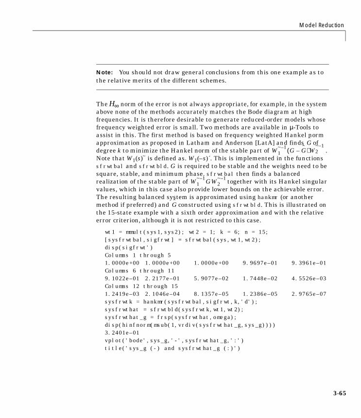
Model Reduction
Note: You should not draw general conclusions from this one example as tothe relative merits of the different schemes.
The H∞ norm of the error is not always appropriate, for example, in the systemabove none of the methods accurately matches the Bode diagram at highfrequencies. It is therefore desirable to generate reduced-order models whosefrequency weighted error is small. Two methods are available in µ-Tools toassist in this. The first method is based on frequency weighted Hankel normapproximation as proposed in Latham and Anderson [LatA] and finds ofdegree k to minimize the Hankel norm of the stable part of .Note that W1(s)~ is defined as. W1(–s)´. This is implemented in the functionssfrwtbal and sfrwtbld. G is required to be stable and the weights need to besquare, stable, and minimum phase. sfrwtbal then finds a balancedrealization of the stable part of together with its Hankel singularvalues, which in this case also provide lower bounds on the achievable error.The resulting balanced system is approximated using hankmr (or anothermethod if preferred) and constructed using sfrwtbld. This is illustrated onthe 15-state example with a sixth order approximation and with the relativeerror criterion, although it is not restricted to this case.
wt1 = mmult(sys1,sys2); wt2 = 1; k = 6; n = 15; [sysfrwtbal,sigfrwt] = sfrwtbal(sys,wt1,wt2); disp(sigfrwt') Columns 1 through 51.0000e+00 1.0000e+00 1.0000e+00 9.9697e–01 9.3961e–01Columns 6 through 119.1022e–01 2.2177e–01 5.9077e–02 1.7448e–02 4.5526e–03Columns 12 through 151.2419e–03 2.1046e–04 8.1357e–05 1.2386e–05 2.9765e–07sysfrwtk = hankmr(sysfrwtbal,sigfrwt,k,'d'); sysfrwthat = sfrwtbld(sysfrwtk,wt1,wt2); sysfrwthat_g = frsp(sysfrwthat,omega); disp(hinfnorm(msub(1,vrdiv(sysfrwthat_g,sys_g)))) 3.2401e–01vplot('bode',sys_g,'-',sysfrwthat_g,':') title('sys_g (-) and sysfrwthat_g (:)')
GW1
~ 1– G G–( )W2~ 1–
W1~ 1– GW2
~ 1–
G
3-65

3 H∞ Control and Model Reduction
3-6
Figure 3-18 Frequency Response of the Original System and Frequency Weighted Balanced Reduction with sfrwtbld
The frequency weighted error is close to the unachievable lower bound ofsigfrwt(k+1). A plot of this is shown in Figure 3-18. You can verify that thismethod is optimal by checking that the Hankel norm of the stable part of theweighted error is sigfrwt(k+1), using sfrwtbal as follows. (Note that theseroutines use sdecomp, which decomposes a system into the sum of two systemswith poles to the left and right of a vertical line in the complex plane.)
[sysfrwterr,sigfrwterr] =...sfrwtbal(msub(sys,sysfrwthat),wt1,wt2); disp(max(sigfrwterr)); 2.2177e–01
A method that is particularly appropriate for relative error model reduction isobtained using srelbal. The error criterion is the same as in the generalfrequency weighted case but with W1 = I and W2 satisfying .This method is related to balanced stochastic truncation as introduced by Desaiand Pal [DesP]. The lower bounds can be obtained as above and upper boundshave been derived by Green [Gre] and improved by Wang and Safonov [WanS].There is no requirement that the system be square or minimum phase but it
10-2
10-1
100
101
102
10-1 100 101 102 103
Log
Mag
nitu
de
Frequency (radians/sec)
-100
0
100
200
10-1 100 101 102 103
Pha
se (
degr
ees)
Frequency (radians/sec)
sys_g (-) and sysfrwthat_g (:)
W2W2~ G~G=
6

Model Reduction
must not have fewer columns than rows. The resulting realization can betruncated as before.
[sysrelbal,sigrel] = srelbal(sys); sysrelbalk = strunc(sysrelbal,k); sysrelbalk_g = frsp(sysrelbalk,omega); disp(hinfnorm(msub(1,vrdiv(sysrelbalk_g,sys_g)))); 4.7480e–01vplot('bode',sys_g,'-',sysrelbalk_g,'--',sysfrwthat_g,':') title('model reduction example: relative error')
Figure 3-19 Frequency Response of the Original System and Reduced Order Models Using Relative Error Methods
It can be checked that sigrel equals sigfrwt above in this case. Both methodsperform well with results close to the lower bound and similar frequencyresponses as seen in Figure 3-19. Glover [Glo2] suggests a combination ofadditive and relative error by performing relative error model reduction of the
augmented system, . Relative error is recovered if α = 0, and additive error
as α → ∞. The resulting approximation can be thought of as satisfying
10-2
10-1
100
101
102
10-1 100 101 102 103
Log
Mag
nitu
de
Frequency (radians/sec)
-100
0
100
200
10-1 100 101 102 103
Pha
se (
degr
ees)
Frequency (radians/sec)
model reduction example: relative error
GαI
3-67

3 H∞ Control and Model Reduction
3-6
where has been made small. This is easily
implemented using srelbal as follows to give a seventh order fit with aperformance between the two extremes.
k = 7; alpha = 15; [sysrelbal,sigrel] = srelbal(abv(sys,alpha*eye(1))); sysrelbalk = sel(strunc(sysrelbal,k),1,1);
You can evaluate the error in the same manner as was done in the frequencyweighted balanced reduction case.
G I( ∆r )G α∆a+ += ∆r ∆a ∞
8

References
References [AdAK:] Adamjan, V.M., D.Z. Arov, and M.G. Krein, “Infinite block Hankelmatrices and related extension problems,” AMS Transl., vol. 111, pp. 133-156,1978.
[And:] Anderson, B.D.O., “An algebraic solution to the spectral factorizationproblem,” IEEE Transactions on Automatic Control, vol. AC-12, pp. 410-414,1967.
[BallC:] Ball, J.A. and N. Cohen, “Sensitivity minimization in an H∞ norm:Parametrization of all suboptimal solutions,” International Journal of Control,vol. 46, pp. 785-816, 1987.
[BallH:] Ball, J.A. and J.W. Helton, “A Beurling-Lax theorem for the Lie groupU(m,n) which contains most classical interpolation theory,” J. Op. Theory, vol.9, pp. 107-142, 1983.
[BamP:] Bamieh, B.A. and J.B. Pearson, “A general framework for linearperiodic systems with applications to H∞ sampled-data control,” IEEETransactions on Automatic Control, vol. AC-37, pp. 418–435, 1992.
[BoyBk:] Boyd, S., V. Balakrishnan, and P. Kabamba, “A bisection method forcomputing the H∞ norm of a transfer matrix and related problems,” Math.Control, Signals, and Systems, vol. 2, no. 3, pp. 207-220, 1989.
[ClemG:] Clements, D.J. and K. Glover, “Spectral Factorization via HermitianPencils,” Linear Algebra and its Applications, Linear Systems Special Issue,pp. 797-846, Sept. 1989.
[DesP:] Desai, U.B. and D. Pal, “A transformation approach to stochastic modelreduction,” IEEE Transactions on Automatic Control, vol. AC-29, pp.1097-1100, 1984.
[Doy1:] Doyle, J.C., “Lecture notes in advances in multivariable control,”ONR/Honeywell Workshop, Minneapolis, 1984.
[DoyFT:] Doyle, J.C. , B.A. Francis, and A.R. Tannenbaum, Feedback ControlTheory, Macmillian Publishing Company, New York, Toronto, 1992.
[DoyGKF:] Doyle, J.C., K. Glover, P. Khargonekar, and B. Francis,“State-space solutions to standard H2 and H∞ control problems,” IEEETransactions on Automatic Control, vol. AC-34, no. 8, pp. 831-847, August1989.
3-69

3 H∞ Control and Model Reduction
3-7
[Enn:] Enns, D., “Model reduction for control system design,” Ph.D.dissertation, Stanford University, June, 1984.
[FoisT:] Foias, C., and A. Tannenbaum, “On the four-block problem, I,” inOperator Theory: Advances and Applications, vol. 32, pp. 93-122, 1988 and “Onthe four-block problem, II: The singular system,” Int. Equations OperatorTheory, vol. 11, pp. 726-767, 1988.
[Fran1:] Francis, B.A., A course in H∞ control theory, Lecture Notes in Controland Information Sciences, vol. 88, Springer-Verlag, Berlin, 1987.
[FranD:] Francis, B.A. and J.C. Doyle, “Linear control theory with an H∞optimality criterion,” SIAM J. Control and Opt., vol. 25, pp. 815-844, 1987.
[GeoS:] T. Georgiou and M. Smith, “Robust stabilization in the gap metric:Controller design for distributed plants,” IEEE Transactions on AutomaticControl, pp. 1133-1143, vol. AC-37., no. 8, Aug. 1992.
[Glo1:] Glover, K., “All optimal Hankel-norm approximations of linearmultivariable systems and their L∞ error bounds,” International Journal ofControl, vol. 39, pp. 1115-1193, 1984.
[Glo2:] K. Glover, “Multiplicative approximation of linear multivariablesystems with L∞ error bounds,” Proceedings of the American ControlConference, Seattle, pp. 1705-1709, 1986.
[Glo3:] Glover, K., “Tutorial on Hankel-norm approximation,” in From Data toModel (J.C. Willems ed.), Springer-Verlag, pp. 26-48, 1989.
[GloD:] Glover, K. and J.C. Doyle, “State-space formulae for all stabilizingcontrollers that satisfy an H∞ norm bound and relations to risk sensitivity,”Systems and Control Letters, vol. 11, pp. 167-172, August 1989. InternationalJournal of Control, vol. 39, pp. 1115–1193, 1984.
[GloD2:] Glover, K. and J. Doyle, “A state-space approach to H∞ optimalcontrol,” in Three Decades of Mathematical Systems Theory: A Collection ofSurveys at the Occasion of the 50th Birthday of Jan C. Willems, H. Nijmeijerand J.M. Schumacher (Eds.), Springer-Verlag Lecture Notes in Control andInformation Sciences vol. 135, 1989.
[GloM:] Glover, K. and D. Mustafa, “Derivation of the Maximum EntropyH∞-controller and a State-space formula for its Entropy,” InternationalJournal of Control, vol. 50, no. 3, pp. 899-916, Sept. 1989.
0

References
[GloLDKS:] Glover, K., D.J.N. Limebeer, J.C. Doyle, E.M. Kasenally, and M.G.Safonov, “A characterization of all solutions to the four block general distanceproblem,” SIAM J. Control and Opt., vol. 29, no. 2, pp. 283-324, March, 1991.
[GohLR:] Gohberg, I., P. Lancaster and L. Rodman, “On the Hermitiansolutions of the symmetric algebraic Riccati equation,” SIAM J. Control andOpt., vol. 24, no. 6, pp. 1323-1334, 1986.
[Gre:] Green, M., “A relative error bound for balanced stochastic truncation,”IEEE Transactions on Automatic Control, vol. AC-33, pp. 961-965, 1988.
[GGLD:] Green, M., K. Glover, D. Limebeer, and J.C. Doyle, “A J-spectralfactorization approach to H∞ control,” SIAM J. Control and Opt., Vol. 28(6), pp.1350-1371, 1990.
[HarK:] Hara, S. and P.T. Kabamba, “On computing the induced norm ofsampled data feedback systems,” Proceedings of the American ControlConference, Green Valley, AZ, pp. 319-320, 1990.
[HauS:] Hautus, M.L.J. and L.M. Silverman, “System structure and singularcontrol.” Linear Algebra Applications, vol. 50, pp. 369-402, 1983.
[Hung:] Hung, Y.S., “RH∞-optimal control-Part I: Model matching, Part II:Solution for controllers,” International Journal of Control, vol. 49, pp. 675-684,1998.
[JonJ:] Jonckheere, E.A., and J.C. Juang, “Fast computation of achievableperformance in mixed sensitivity H∞ design,” IEEE Transactions on AutomaticControl, vol. AC-32, pp. 896-906, 1987.
[KabH:] Kabamba, P.T. and S. Hara, “Worst case analysis and design ofsampled data control systems,” IEEE Transactions on Automatic Control, vol.AC-38, no. 9, pp. 1337-1357, Sept. 1993.
[KhaPZ:] Kargoneckar, P.P., I.R. Peterson, and M.A. Rotea, “H∞ optimalcontrol with state-feedback,” IEEE Transactions on Automatic Control, vol.AC-33, pp. 786-788, 1988.
[Kim:] Kimura, H., “Synthesis of H∞ controllers based on conjugation,”Proceedings of IEEE Conference on Decision and Control, Austin, TX., pp.1207-1211, 1988.
[Kwak:] Kwakernaak, H., “A polynomial approach to minimax frequencydomain optimization of mutlivariable feedback systems,” InternationalJournal of Control, pp. 117-156, 1986.
3-71

3 H∞ Control and Model Reduction
3-7
[Kuc1:] Kucera V., “A contribution to matrix quadratic equations,” IEEETransactions on Automatic Control, vol. AC-17, no. 3, pp. 344-347, 1972.
[LatA:] Latham, G.A. and B.D.O. Anderson, “Frequency-weighted optimalHankel norm approximation of state transfer functions,” Systems and ControlLetters, vol. 5, pp. 229-236, 1985.
[LimH:] Limebeer, D.J.N. and G.D. Halikias, “A controller degree bound forH∞-optimal control problems of the second kind,” SIAM J. Control and Opt.,vol. 26, no. 3, pp. 646-677, 1988.
McFG1:] McFarlane, D.C. and K. Glover, Robust Controller Design usingNormalised Coprime Factor Plant Descriptions, Springer-Verlag Lecture Notesin Control and Information Sciences, vol. 138, 1989.
[McFG2:] McFarlane, D.C. and K. Glover, “A Loop Shaping Design Procedureusing H∞ Synthesis,” IEEE Transactions on Automatic Control, vol. AC-37, no.6, pp. 759-769, June 1992.
[Moo:] Moore, B.C., “Principal components analysis in linear systems:controllability, observability and model reduction,” IEEE Transactions onAutomatic Control, vol. AC-26, pp. 17-31, 1981.
[MusG:] Mustafa, D. and K. Glover, “Controllers which satisfy a closed-loop H∞norm bound and maximize an entropy integral,” Proceedings of the 27th IEEEConference on Decision and Control, Austin, Texas, 1988, pp. 1609-1613.
[QiuD:] Qiu, L. and E.J. Davison, “Feedback stability under simultaneous gapmetric uncertainties in plant and controller,” Systems & Control Letters, vol.18(1), pp. 9-22, 1992.
[Red:] Redheffer, R.M., “Inequalities for a matrix Riccati equation,” Journal ofMathematics and Mechanics, vol. 8, no. 3, pp. 349-367, 1959.
[Red2:] Redheffer, R.M., “On a certain linear fractional transformation,”Journal of Mathematics and Physics, vol. 39, pp. 269-286, 1960.
[SafCL:] Safonov, M.G., R.Y. Chiang and D.J.N. Limebeer, “Hankel modelreduction without balancing: a descriptor approach,” Proceedings of the 26thIEEE Conference on Decision and Control, Los Angeles, 1987.
[SafLC:] Safonov, M.G., D.J.N. Limebeer, and R.Y. Chiang, “Simplifying theH∞ theory via loop shifting,” Proceedings of the 27th IEEE Conference onDecision and Control, vol. 2, pp. 1399-1404, 1989.
2
References
[Sara:] Sarason, D., “Generalized interpolation in H∞,” AMS. Trans., vol. 127,pp. 179-203, 1967.
[Silv:] Silverman, L.M., “Inversion of multivariable linear systems,” IEEETransactions on Automatic Control, vol. AC-14, pp. 270-276, 1969.
[Toi:] Toivonen, H.T., “Sampled-data control of continuous-time systems withan H∞ optimality criterion,” Report 90-1, Dept. of Chemical Engineering, AboAkademi, Finland, Jan., 1990.
[VanD:] Van Dooren, P., “A generalized eigenvalue approach for solving Riccatiequations,” SIAM J. Sci. Comput., vol. 2, pp. 121-135, 1981.
[Vin:] Vinnicombe, G., “Measuring Robustness of Feedback Systems,” PhDdissertation, Department of Engineering, University of Cambridge, 1993.
[WanS:] Wang, W. and M.G. Safonov, “A tighter relative error bound forbalanced stochastic truncation,” Systems and Control Letters , vol. 14, pp.307-317, 1990.
[Will1:] Willems, J.C., “Least-squares stationary optimal control and thealgebraic Riccati equation,” IEEE Transactions on Automatic Control, vol.AC-16, pp. 621-634, 1971.
[Will2:] Willems, J.C., “Almost invariant subspaces: an approach to high gainfeedback design – Part I: almost controlled invariant subspaces.” IEEETransactions on Automatic Control, vol. AC-26, pp. 235-252, 1981.
[WilKS:] Willems, J.C., A. Kitapci and L.M. Silverman, “Singular optimalcontrol: a geometric approach.” SIAM J. Control and Opt., vol. 24, pp. 323-337,1986.
[Wonh:] Wonham, W.M., Linear Multivariable Control: A Geometric Approach,third edition, Springer-Verlag, New York, 1985.
[YouJB:] Youla, D.C., H.A. Jabr, and J.J. Bongiorno, “Modern Wiener-Hopfdesign of optimal controllers: part II,” IEEE Transactions on AutomaticControl, vol. AC-21, pp. 319-338, 1976.
[Yam:] Yamamamoto, Y., “A new approach to sampled-data control systems—A function space viewpoint with applications to tracking problems,”Proceedings of the 29th Conference on Decision and Control, pp. 1882-1887,1990.
3-73

3 H∞ Control and Model Reduction
3-7
[Zame:] Zames, G., “Feedback and optimal sensitivity: model referencetransformations, multiplicative seminorms, and approximate inverses,” IEEETransactions on Automatic Control, vol. AC-26, pp. 301-320, 1981.
[ZamE:] Zames, G. and El-Sakkary, “Unstable systems and feedback: The gapmetric,” Proceedings of the Allerton Conference, pp. 380-385, Oct., 1980.
[ZhoK:] Zhou, K., and P.P. Khargoneckar, “An algebraic Riccati equationapproach to H∞ optimization,” Systems and Control Letters, vol. 11, pp. 85-92,1988.
4

4
Modeling and Analysis ofUncertain Systems
4 Modeling and Analysis of Uncertain Systems
4-2
The advanced features of the µ-Analysis and Synthesis Toolbox (µ-Tools) areaimed at
• Analyzing the effect of uncertain models on achievable closed-loopperformance
• Designing controllers to provide optimal worst-case performance in the faceof the plant uncertainty
Hence, it is imperative that you understand
• How model uncertainty is represented in this framework
• The technical tools available to answer questions about the robustness of agiven closed-loop system to certain forms of model uncertainty
In this chapter, we concentrate on these ideas, through concepts of linearfractional transformations and the structured singular value (µ). We begin inthe next section with linear fractional transformations (LFTs) and their role inmodeling uncertainty in matrices and systems.
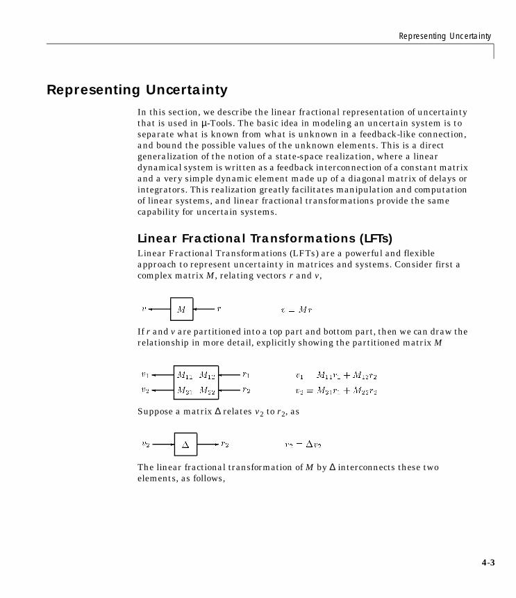
Representing Uncertainty
Representing UncertaintyIn this section, we describe the linear fractional representation of uncertaintythat is used in µ-Tools. The basic idea in modeling an uncertain system is toseparate what is known from what is unknown in a feedback-like connection,and bound the possible values of the unknown elements. This is a directgeneralization of the notion of a state-space realization, where a lineardynamical system is written as a feedback interconnection of a constant matrixand a very simple dynamic element made up of a diagonal matrix of delays orintegrators. This realization greatly facilitates manipulation and computationof linear systems, and linear fractional transformations provide the samecapability for uncertain systems.
Linear Fractional Transformations (LFTs)Linear Fractional Transformations (LFTs) are a powerful and flexibleapproach to represent uncertainty in matrices and systems. Consider first acomplex matrix M, relating vectors r and v,
If r and v are partitioned into a top part and bottom part, then we can draw therelationship in more detail, explicitly showing the partitioned matrix M
Suppose a matrix ∆ relates v2 to r2, as
The linear fractional transformation of M by ∆ interconnects these twoelements, as follows,
M v r v =Mr
M11 M12
M21 M22
v1
v2
r1
r2
v1 =M11r1 +M12r2
v2 =M21r1 +M22r2
- -v2 r2 r2 = v2
4-3

4 Modeling and Analysis of Uncertain Systems
4-4
Eliminate v2 and r2, leaving the relationship between r1 and v1
The notation FL indicates that the lower loop of M is closed with ∆. It is moretraditional to write a block diagram with the arrows reversed, as in
This still represents the same formula, v1 = FL(M,∆)r1, and the choice ofdirections is a matter of taste. We prefer to write as much as is convenient of ablock diagram with the arrows going right to left to be consistent with matrixand operator composition, which goes the same way. This simple conventionreduces the confusion in going between block diagrams and equations,particularly when blocks have multiple inputs.
If the upper loop of M is closed with Ω, then we have
-
M11 M12
M21 M22
v1 r1
v1 M11 M12∆ I M22∆–( ) 1– M21+[ ]r1=
FL M ∆,( )r1=
FL M ∆,( )
M
--
-
r1 v1
-
M11 M12
M21 M22v2 r2
v2 = FU (M;) r2

Representing Uncertainty
where
FU(M,Ω) := [M22 + M21Ω(I – M11Ω)–1M12]
Parametric UncertaintyHow do we use LFTs to represent an uncertain parameter? Suppose c is aparameter, and it is known to take on values
Write this as c = 2.4+0.4δc where δc ∈ [–1,1]. This is a linear fractionaltransformation. Indeed, check that
So, everywhere ← ← appears in a block diagram, simply replace it with
If the gain c–1 also appears, the LFT representation can still be used, becauseinverses of LFTs are LFTs (on the same δ). Note that
So, everywhere← ← appears in a block diagram, replace it with
c FL2.4 0.41 0
δc,
=
c
c
-
2:4 0:4
1 0
12.4--------
16---– δc
1 16---–( )–
-------------------δc
+=
c 1– 12.4 0.4δc+----------------------------=
FL
12.4-------- 0.4–
12.4-------- 1
6---–
δc,
=
1c---
4-5

4 Modeling and Analysis of Uncertain Systems
4-6
The general case for inverses can be solved with the matrix inversion lemma.Specifically, given a matrix H, there exists matrices HLI and HUI such that forall ∆ and Ω
[FL(H,∆)]–1 = FL(HLI,∆), [FU(H,Ω)]–1 = FU(HUI,Ω)
In fact, with , the formulas for HLI and HUI are just
Consider a second order system, representing a single degree-of-freedom mass/damper/spring system with uncertain elements
The coefficients are assumed to be uncertain, with a nominal value, and arange of possible variation
with –1 ≤ δm, δc, δk ≤ 1. Note that this represents 50% uncertainty in m, 30%uncertainty in c, 40% uncertainty in k. A block diagram is shown in Figure 4-1.
c
-
1
2:4:4
1
2:4
1
6
HH11 H12
H21 H22
=
HLIH11
1– H– 111– H12
H21H111– H22 H21H11
1– H12–=
HLIH11 H12H22
1– H21– H12H221–
H– 221– H21 H22
1–=
mx cx· kx+ + u=..
m m 1 0.5δm+( ),= c c 1 0.3δc+( ),= k k 1 0.4δk+( )=
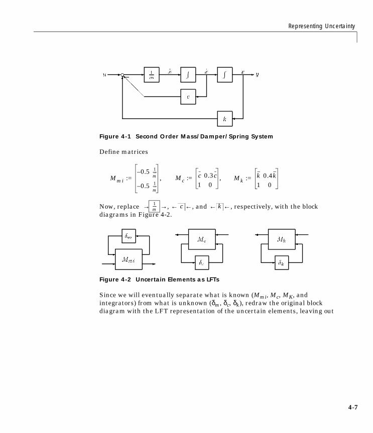
Representing Uncertainty
Figure 4-1 Second Order Mass/Damper/Spring System
Define matrices
Now, replace → →, ← ←, and ← ←, respectively, with the blockdiagrams in Figure 4-2.
Figure 4-2 Uncertain Elements as LFTs
Since we will eventually separate what is known (Mmi, Mc, MK, andintegrators) from what is unknown (δm, δc, δk), redraw the original blockdiagram with the LFT representation of the uncertain elements, leaving out
1
m
R R
k
c
- c
- - -
@@
@@I-
6x _x xu y
Mc := c 0.3c1 0
,Mmi :=0.5– 1
m-----
0.5– 1m-----
, Mk := k 0.4k1 0
1m----- c k
4-7

4 Modeling and Analysis of Uncertain Systems
4-8
the δs, but label the signals which go to and from the δs. This is shown in Figure4-3.
Figure 4-3 Known Part of Uncertain System
Let Gmck be the four-input (wm, wc, wk, u), four-output (zm, zc, zk, y), two-statesystem shown in Figure 4-3 and depicted in Figure 4-4.
Figure 4-4 Macro View of Known System
Note that Gmck only depends on , 0.5, 0.4, and 0.3 and the originaldifferential equation which relates u to y. Hence, Gmck is known. Also, theuncertain behavior of the original system is characterized by an upper linearfractional transformation, FU, of Gmck with a diagonal uncertainty matrix asshown in Figure 4-5.
R R- c
- - -
@@@I
-
6
Mk wkzk
Mc wczc
Mmi
- -wm zm
x _x xu y
Gmck
zmzczky
wmwcwku
m , c, k,
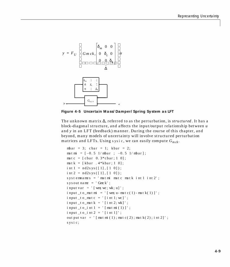
Representing Uncertainty
Figure 4-5 Uncertain Mass/Damper/Spring System as LFT
The unknown matrix ∆, referred to as the perturbation, is structured. It has ablock-diagonal structure, and affects the input/output relationship between uand y in an LFT (feedback) manner. During the course of this chapter, andbeyond, many models of uncertainty will involve structured perturbationmatrices and LFTs. Using sysic, we can easily compute Gmck.
mbar = 3; cbar = 1; kbar = 2; matmi = [–0.5 1/mbar ; –0.5 1/mbar]; matc = [cbar 0.3*cbar;1 0]; matk = [kbar .4*kbar;1 0]; int1 = nd2sys([1],[1 0]); int2 = nd2sys([1],[1 0]); systemnames = 'matmi matc matk int1 int2'; sysoutname = 'Gmck'; inputvar = '[wm;wc;wk;u]'; input_to_matmi = '[wm;u-matc(1)-matk(1)]'; input_to_matc = '[int1;wc]'; input_to_matk = '[int2;wk]'; input_to_int1 = '[matmi(1)]'; input_to_int2 = '[int1]'; outputvar = '[matmi(1);matc(2);matk(2);int2]'; sysic;
Gmck
m 0 0
0 c 0
0 0 k
y
-
u
y FU= Gmck
δm 0 0
0 δc 0
0 0 δk
,
∆
u
4-9

4 Modeling and Analysis of Uncertain Systems
4-1
µ-Tools Commands for LFTsThe lower and upper LFT formulas are implemented in µ-Tools with thecommand starp. The name starp comes from the star product operationdefined and developed in [Red1]. The star product is a generalization of theLFT, and includes both the lower and upper LFTs as special cases.
Suppose that T and B are two matrices (CONSTANT, VARYING or SYSTEM)partitioned as below.
such that the matrix product T22B11is well defined, and in fact, square.
If I – T22B11 is invertible, define the star product of T and B to be
where FL and FU are defined as earlier,
In a block diagram, the star product appears as
and would be computed
S = starp(T,B,n1,n2)
TT11 T12
T21 T22
= , BB11 B12
B21 B22
=
S T B,( ) :=FL T B11,( ) T12 I B11T22–( ) 1– B12
B21 I T22B11–( ) 1– T21 FU B T22,( )
FL T B11,( ) T11 T12B11 I T22B11–( ) 1– T21+=
FU B T22,( ) B22 B21T22 I B11T22–( ) 1– B12+=
B
T
S
n1
n2
XX
XXX
0

µ-Tools Commands for LFTs
Here n1 is the row dimension of [T21 T22] (and the column dimension of ),
which is the number of signals which are fed from T to B. Similarly, n2 is the
row dimension of [B11 B12] (and the column dimension of ), which is the
number of signals which are fed from B to T. The remaining inputs and outputsappear in the output matrix S in the same order as they are in T and B. If thedimension arguments n1 and n2 are omitted, then the following takes place:
• n1 = min([ynum(T) unum(B)])
• n2 = min([unum(T) ynum(B)])
so all possible loop closures are made. Hence, LFTs (which are special cases ofstar products) are easily computed using starp without dimension arguments.
M = crandn(10,8); Delta = crandn(3,4); Omega = crandn(6,3); flmd = starp(M,Delta); fumo = starp(Omega,M);
It is possible to form the star product of two dynamical systems, and it ispossible to form the star product of their frequency responses. Hence, starpworks with all µ-Tools data types.
We can illustrate this by considering the frequency response of the uncertainmass/damper/spring system considered in the previous section entitled“Parametric Uncertainty”. Compute the frequency response of the four-input,four-output system Gmck. Then, the frequency response of the uncertain system
B11
B21
T12
T22
4-11

4 Modeling and Analysis of Uncertain Systems
4-1
is simply the linear fractional transformation of the frequency response of Gmckwith the perturbation matrix (δm, δc, δk).
Gmck_g = frsp(Gmck,logspace(–1,1,100)); delnom = diag([0;0;0]); rifd(spoles(starp(delnom,Gmck))) delnpn = diag([–1;1;–1]); rifd(spoles(starp(delnpn,Gmck))) delpnp = diag([1;–1;1]); rifd(spoles(starp(delpnp,Gmck))) vplot('bode',starp(delnom,Gmck_g),'-',...
starp(delnpn,Gmck_g),'.-',starp(delpnp,Gmck_g),'--')
101
100
101
200
100
0
Pha
se (
degr
ees)
Frequency (radians/sec)
Frequency Response Phases of Perturbed MCK System
101
100
101
104
102
100
102
Log
Mag
nitu
de
Frequency (radians/sec)
Frequency Response Magnitudes of Perturbed MCK System
2

Interconnections of LFTs
Interconnections of LFTs By now, you probably have noticed an extremely important property of LFTs— typical algebraic operations such as frequency response, cascadeconnections, parallel connections, and feedback connections preserve the LFTstructure. This means that normal interconnections of LFTs are still in theform of an LFT. Hence, the LFT is an excellent choice for a general hierarchicalrepresentation of uncertainty. For illustrative purposes, we consider a fewadditional examples in this section.
Consider a cascade connection of FL(M,∆) with FU(G,Ω), so that y =FL(M,∆)FU(G,Ω)u. This is shown below.
Draw a box around M and G, isolating them from ∆ and Ω, calling the boxeditems Q.
Q is made up of the elements of M and G, and relates the variables (u, w∆, wΩ)to (y, z∆, zΩ)
4-13
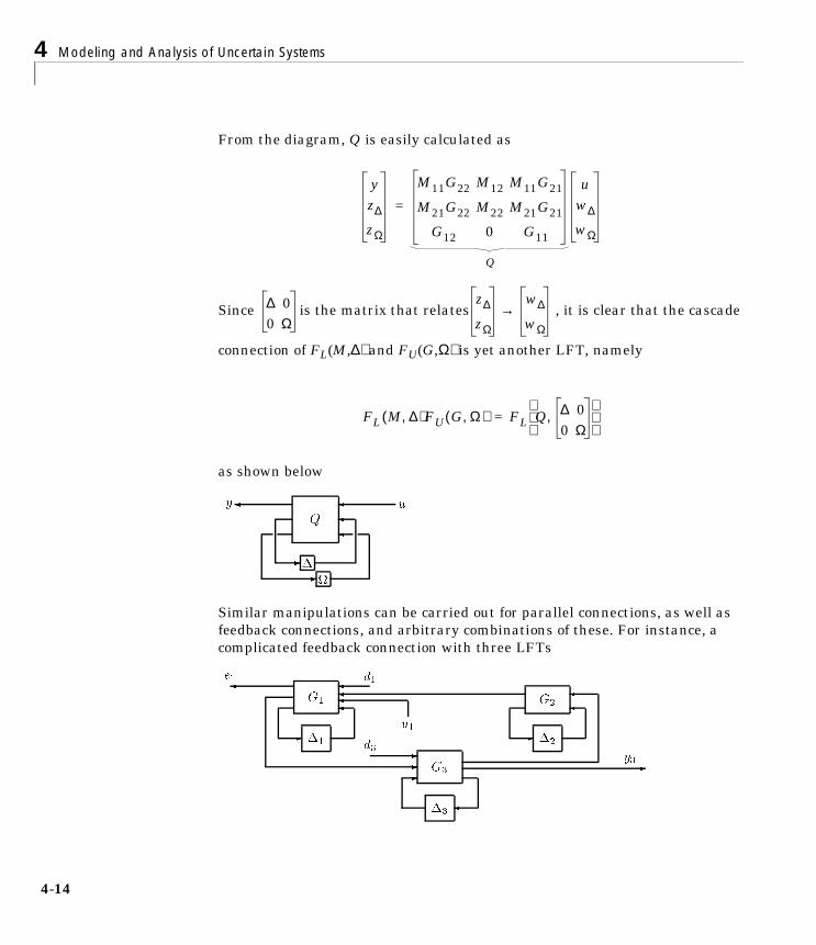
4 Modeling and Analysis of Uncertain Systems
4-1
From the diagram, Q is easily calculated as
Since is the matrix that relates , it is clear that the cascade
connection of FL(M,∆) and FU(G,Ω) is yet another LFT, namely
as shown below
Similar manipulations can be carried out for parallel connections, as well asfeedback connections, and arbitrary combinations of these. For instance, acomplicated feedback connection with three LFTs
yz∆
zΩ
M11G22 M12 M11G21
M21G22 M22 M21G21
G12 0 G11
uw∆
wΩ
=
Q
∆ 00 Ω
z∆
zΩ
w∆
wΩ→
FL M ∆,( )FU G Ω,( ) FL Q ∆ 00 Ω
,
=
Q
y u
-
-
G1
G3
G2
1 2
3
- -
-
- -
-
e1 d1
u1
d3y3
4
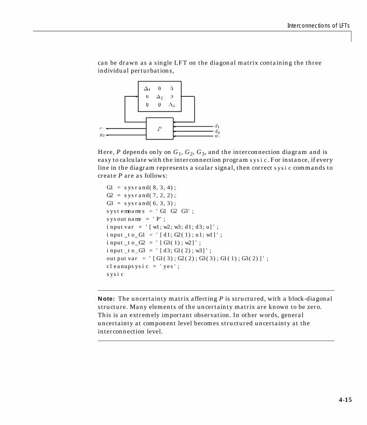
Interconnections of LFTs
can be drawn as a single LFT on the diagonal matrix containing the threeindividual perturbations,
Here, P depends only on G1, G2, G3, and the interconnection diagram and iseasy to calculate with the interconnection program sysic. For instance, if everyline in the diagram represents a scalar signal, then correct sysic commands tocreate P are as follows:
G1 = sysrand(8,3,4); G2 = sysrand(7,2,2); G3 = sysrand(6,3,3); systemnames = 'G1 G2 G3'; sysoutname = 'P'; inputvar = '[w1;w2;w3;d1;d3;u]'; input_to_G1 = '[d1;G2(1);u1;w1]'; input_to_G2 = '[G3(1);w2]'; input_to_G3 = '[d3;G1(2);w3]'; outputvar = '[G1(3);G2(2);G3(3);G1(1);G3(2)]'; cleanupsysic = 'yes'; sysic
Note: The uncertainty matrix affecting P is structured, with a block-diagonalstructure. Many elements of the uncertainty matrix are known to be zero.This is an extremely important observation. In other words, generaluncertainty at component level becomes structured uncertainty at theinterconnection level.
4-15
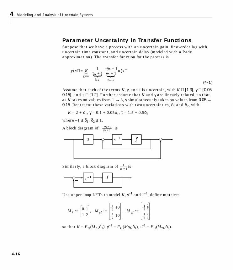
4 Modeling and Analysis of Uncertain Systems
4-1
Parameter Uncertainty in Transfer FunctionsSuppose that we have a process with an uncertain gain, first-order lag withuncertain time constant, and uncertain delay (modeled with a Padeapproximation). The transfer function for the process is
(4-1)
Assume that each of the terms K, γ, and τ is uncertain, with K ∈ [1 3], γ ∈ [0.05 0.15], and τ ∈ [1 2]. Further assume that K and γ are linearly related, so thatas K takes on values from 1 → 3, γ simultaneously takes on values from 0.05 → 0.15. Represent these variations with two uncertainties, δ1 and δ2, with
K = 2 + δ1, γ = 0.1 + 0.05δ1, τ = 1.5 + 0.5δ2
where –1 ≤ δ1, δ2 ≤ 1.
A block diagram of is
Similarly, a block diagram of is
Use upper-loop LFTs to model K, γ–1 and τ–1, define matrices
so that K = FU(MK,δ1), γ–1 = FU(MγI,δ1), τ–1 = FU(MτI,δ2).
y s( ) K 1τs 1+---------------
γs 1+–γs 1+
------------------u s( )=gain
lag Pade
γs– 1+
γs 1+-------------------
1τs 1+---------------
Mk := 0 11 2
, MγI :=12---– 10
12---– 10
, MτI :=13---–
23---
13---–
23---
6

Interconnections of LFTs
The first-order Pade system is of the form FU(GP,δ1), and the first-order lag isof the form FU(GL,δ2), where GP and GL are known, two-input, two-output,one-state systems
GP is shown in detail in Figure 4-6 and can be built easily using sysic.
Figure 4-6 LFT System Gp for Uncertain Pade
For instance
mgammai = [–0.5 10; –0.5 10]; int = nd2sys([1],[1 0]); systemnames = 'mgammai int'; sysoutname = 'GP'; inputvar = '[w_gamma;u1]'; input_to_mgammai = '[w_gamma;2*u1-int]'; input_to_int = '[mgammai(2)]'; outputvar = '[mgammai(1);int-u1]'; sysic;
4-17

4 Modeling and Analysis of Uncertain Systems
4-1
Similar calculations are necessary for GL, whose internal structure is shown inFigure 4-7.
mtaui = [–1/3 2/3; –1/3 2/3]; int = nd2sys([1],[1 0]); systemnames = 'mtaui int'; sysoutname = 'GL'; inputvar = '[w_tau;u2]'; input_to_mtaui = '[w_tau;u2-int]'; input_to_int = '[mtaui(2)]'; outputvar = '[mtaui(1);int]'; sysic;
Figure 4-7 LFT System GL for Uncertain Lag
The uncertain K is directly represented using FU(MK,δ1). The known part ofthe uncertain gain/lag/Pade system is simply a four-input, four-output,two-state system Gproc shown in Figure 4-8 with internal structure shown inFigure 4-9.
Figure 4-8 Known Part of Uncertain Gain/Lag/Pade
Figure 4-9 Cascade of Pade, Lag, and Gain LFTs
Gproc
z zkzy
w
wk
w
u
GP GL MK
-
u- - - - -
y
?
w
- 6
6z
?
w
- 6
6z
?
wk
- 6
6zk
8
Interconnections of LFTs
The uncertain system’s behavior, equation (4-1), is an LFT,
The perturbation δ1 is repeated twice, due to the coupled variation in K and γ.
The SYSTEM matrix Gproc can be constructed with sysic as follows:
MK = [0 1;1 2]; systemnames = 'GP GL MK'; sysoutname = 'Gproc'; inputvar = '[w_gamma;w_k;w_tau;u]'; input_to_GP = '[w_gamma;u]'; input_to_GL = '[w_tau;GP(2)]'; input_to_MK = '[w_k;GL(2)]'; outputvar = '[GP(1);MK(1);GL(1);MK(2)]'; sysic;
We can do some time-domain simulations to verify that this model is correct.Recall that δ1 = –1 translates into K = 1, γ = 0.05 while δ1 = 1 means K = 3,γ = 0.15. Also, δ2 = –1 corresponds to τ = 1, and δ2 = 1 corresponds to τ = 2.
% pertnom ---> nominal values pertnom = diag([0,0,0]); % pert1 ---> low gain, short delay, slow lag pert1 = diag([–1,–1,–1]); % pert2 ---> low gain, short delay, fast lag pert2 = diag([–1,–1,1]); % pert3 ---> high gain, long delay, slow lag pert3 = diag([1,1,–1]); % pert4 ---> high gain, long delay, fast lag pert4 = diag([1,1,1]); tfinal = 4; sysnom = starp(pertnom,Gproc); ynom = trsp(sysnom,1,tfinal); y1 = trsp(starp(pert1,Gproc),1,tfinal); y2 = trsp(starp(pert2,Gproc),1,tfinal); y3 = trsp(starp(pert3,Gproc),1,tfinal); y4 = trsp(starp(pert4,Gproc),1,tfinal);vplot(ynom,'-',y1,':',y2,'–.',y3'--',y4,'+')
y FU Gproc ,δ1I2 0
0 δ2
u=
4-19

4 Modeling and Analysis of Uncertain Systems
4-2
Linear State-Space UncertaintyFor general parametric uncertainty in state-space or transfer function models,the methods outlined in the previous section are used. In the special case oflinear uncertainty in a state-space model, the uncertainty description can bebuilt up even more easily. Consider an uncertain state-space model,
(4-2)
where for each i = 1,2,. . .,m
0 0.5 1 1.5 2 2.5 3 3.5 40.5
0
0.5
1
1.5
2
2.5
Out
put
Time
x· t( )y t( )
A0 δiAi
i 1=
m
∑+ B0 δiBi
i 1=
m
∑+
C0 δiCi
i 1=
m
∑+ D0 δiDi
i 1=
m
∑+
x t( )u t( )
=
A0 B0
C0 D0
δiAi Bi
Ci Dii
m
∑+
x t( )u t( )
=
0

Interconnections of LFTs
Let
and factor each matrix (using svd, for instance) as
where
Now, define a linear system Gss, with extra inputs and outputs via the stateequations
Ai Bi
Ci Di
Rn+nu( ) n+ny( )×
∈
ri := rankAi Bi
Ci Di
Ai Bi
Ci Di
Ei
FiGi Hi=
Ei
Fi
Rn+ny( ) ri×
∈ , Gi Hi Rri n+ny( )×
∈
x·
u
z1
zm
A0 B0 E1 … Em
C0 D0 F1 … Fm
G1 H1 0 … 0
Gm Hm 0 … 0
x
u
w1
wm
=
… …… … … …...
4-21

4 Modeling and Analysis of Uncertain Systems
4-2
Figure 4-10 Linear System: Gss
as shown in Figure 4-10.
The uncertain system in equation (4-2) is represented as an LFT around Gss,namely
y = FL(Gss,∆)u
where ∆ maps z → w, and has the structure given as
∆ = diag[δ1 ,. . .,δm ] : δi ∈ R
This approach, developed in [MorM], has its roots in the Gilbert realization,which is discussed in [Kai].
As an example, consider a two-state, single-input, single-output system with asingle parameter dependence,
The matrix multiplying δ has rank 1, and factors simply as
Gss
yz1z2
zm
uw1
w2
wm
Ir1Irm
A δ( ) B δ( )C δ( ) D δ( )
:=0 1 0
16– 0.16– 116 0 0
δ0 0 0
6.4 0 00 0 0
+
0 0 06.4 0 0
0 0 0
06.4
01 0 0=
2

Interconnections of LFTs
so the state equations for Gss are
Unmodeled DynamicsModels of uncertainty are not limited to parametric uncertainty. Often, a loworder, nominal model, which suitably describes the low-mid frequency rangebehavior of the plant is available, but the high-frequency plant behavior isuncertain. In this situation, even the dynamic order of the actual plant is notknown, and something richer than parametric uncertainty is needed torepresent this uncertainty. One common approach for this type of uncertaintyis to use a multiplicative uncertainty model. Roughly, this allows you to specifya frequency-dependent percentage uncertainty in the actual plant behavior.
In order to specify the uncertainty set, we need to choose two things:
• A nominal model, G(s)
• A multiplicative uncertainty weighting function, Wu(s)
Given these, the precise definition of the multiplicative uncertainty set is
with the additional restriction that the number of right-half plane (RHP) polesof be equal to the number of right-half plane poles of G. At each frequency,|Wu(jω)| represents the maximum potential percentage difference between allof the plants represented by M(G,Wu) and the nominal plant model G. In thatsense, M(G,Wu) represents a ball of possible plants, centered at G. On aNyquist plot, a disk of radius |Wu(jω)G(jω)|, centered at G(jω) is the set ofpossible values that can take on, due to the uncertainty description.
x·1
x·2
u
z1
0 1 0 016– .16– 1 6.416 0 0 0
1 0 0 0
x1
x2
u
w1
=
M G Wu,( ) := G : G jω( ) G jω( )–G jω( )
-------------------------------------- Wu jω( )≤
G
G jω( )
4-23
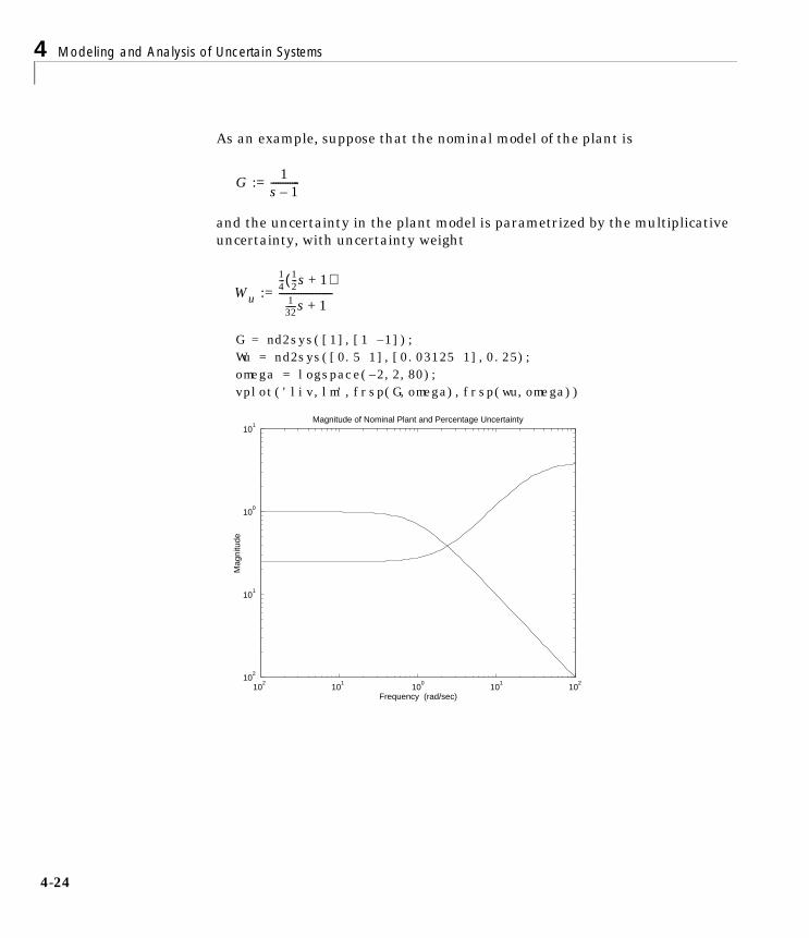
4 Modeling and Analysis of Uncertain Systems
4-2
As an example, suppose that the nominal model of the plant is
and the uncertainty in the plant model is parametrized by the multiplicativeuncertainty, with uncertainty weight
G = nd2sys([1],[1 –1]); Wu = nd2sys([0.5 1],[0.03125 1],0.25); omega = logspace(–2,2,80); vplot('liv,lm',frsp(G,omega),frsp(wu,omega))
G := 1s 1–------------
Wu :=14---
12---s 1+( )
132------s 1+
----------------------
102
101
100
101
102
102
101
100
101
Magnitude of Nominal Plant and Percentage Uncertainty
Frequency (rad/sec)
Mag
nitu
de
4

Interconnections of LFTs
It is instructive to consider sets of models that are similar to the nominal modelG, and see to what extent the sets are contained in M(G,Wu). Consider thefollowing problem. Determine the smallest such that
The easiest approach using µ-Tools is just to compute, and plot
for various values of β, and determine the lower limit by comparing the plot’smagnitude relative to 1. Using the command ex_unc, it is easy to carry out thisprocedure. For instance,
beta = 1; Gtilde = mmult(nd2sys(beta,[1 beta]),G) ex_unc(G,Gtilde,wu,omega); % above 1 beta = 10; Gtilde = mmult(nd2sys(beta,[1 beta]),G)ex_unc(G,Gtilde,wu,omega); % below 1
file: ex_unc.m function ex_unc(G,Gtilde,Wu,omega) Gg = frsp(G,omega); Gtildeg = frsp(Gtilde,omega); Wug = frsp(Wu,omega); percdiff = vabs(vrdiv(msub(Gtildeg,Gg),mmult(Gg,Wug)));vplot('liv,m',percdiff,1);
β
Gβ
s β+------------ : β β>
M G Wu,( )⊂
G jω( ) G jω( )–G jω( )Wu jω( )--------------------------------------
β
4-25

4 Modeling and Analysis of Uncertain Systems
4-2
A few more trials reveal As an exercise, carry out similar calculationson the following examples:
• Define and as the smallest and largest numbers such that
Exercise: Using µ-Tools, show that and .
• Define as the largest number such that
Exercise: Using µ-Tools, show .
• Define and as the smallest and largest numbers such that
Exercise: Using µ-Tools, show that and .
• Define as the largest integer such that
Exercise: Using µ-Tools, show .
We return to this example, and these specific extreme plants later in the“Analysis of Controllers for an Unstable System” section in Chapter 7.
Now, by defining , each can be drawn as in Figure 4-11.
β 6.1.≈
δ 0> δ 0>
1 δ+s 1– δ–-------------------- : δ δ δ≤ ≤
M G Wu,( )⊂
δ 0.33≈ δ 0.425≈
τ 0>
G τs– 1+τs 1+
------------------- : τ τ≤
M G Wu,( )⊂
τ 0.07≈
r 0> r 0>
G702
s2 2ξ70s 702+ +
-------------------------------------------- : ξ ξ ξ≤ ≤
M G Wu,( )⊂
ξ 0.145≈ ξ 5.7≈
m 0>
G 50s 50+---------------
m: m 0,1,…,m=
M G Wu,( )⊂
m 6=
∆ := G G–GWu--------------- G
6

Interconnections of LFTs
Figure 4-11 Multiplicative Uncertainty
In order to satisfy the constraint , ∆ must be a transfer functionthat satisfies , and
#RHP poles [G(1 + Wu∆)] = #RHP poles [G]
Note that ∆ itself may be unstable — reconsider the previous exampleinvolving the parameter δ. There, the unstable pole of changes location. It iseasy to verify that
(4-3)
gives (by simple algebraic manipulation)
as desired. Moreover, the ∆'s that actually yield
G(1 + Wu∆) ∈ M(G,Wu)
are those in equation (4-3) which also satisfy
-u 6
Wu
-
?- G - yf+
+
Behavior ofplants inM(G;Wu)
G M G Wu,( )∈max ∆ jω( ) 1≤
ω
G
∆1
32------ s 1+( )δs
14---
12---s 1+( ) s 1– δ–( )
-------------------------------------------------=:
G 1 Wu∆+( ) 1s 1–------------ 1
14--- 1
2---s 1+( )
132------s 1+( )
----------------------∆+
=
s 1–( ) 1 δ+( )s 1–( ) s 1– δ–( )
-------------------------------------------=
1 δ+s 1– δ–--------------------=
max ∆ jω( ) 1≤ω R∈
4-27

4 Modeling and Analysis of Uncertain Systems
4-2
It is important to understand that in this situation, ∆, G, and Wu are not viewedas three separate physical devices which are interconnected to form . If theywere, then the interconnection in Figure 4-11 would actually have two unstablemodes, at (1) and (1 + δ), but the mode at 1 would be uncontrollable from u.Obviously, no controller could internally stabilize the system. Instead, ∆, G,and Wu are just combined to yield a useful manner (through the definition ofM(G,Wu)) to parametrize a set of plants that are similar (in a precise way) to G.
As usual, we represent the uncertain plant set M(G,Wu) as an LFT byseparating the known elements (G and Wu) from the unknown elements (∆) asshown in the following figure.
The uncertain component is now represented as y = FU(Hmult,∆)u, with Hmulthaving the value
Hmult is easily calculated using sysic or simpler manipulations.
Hmult = madd(mmult([1;0],wu,[0 1]),mmult([0;1],G,[1 1])); % or systemnames = 'wu G'; sysoutname = 'Hmult'; inputvar = '[w;u]'; input_to_wu = '[u]'; input_to_G = '[w+u]'; outputvar = '[wu;G]'; sysic
G
--
6?
-u 6
Wu
z
-
?
w
- G - yf+
+
Hmult
Known, 2-input,2-output, linearsystem
zy
0 Wu
G G
wu
=
Hmult
8
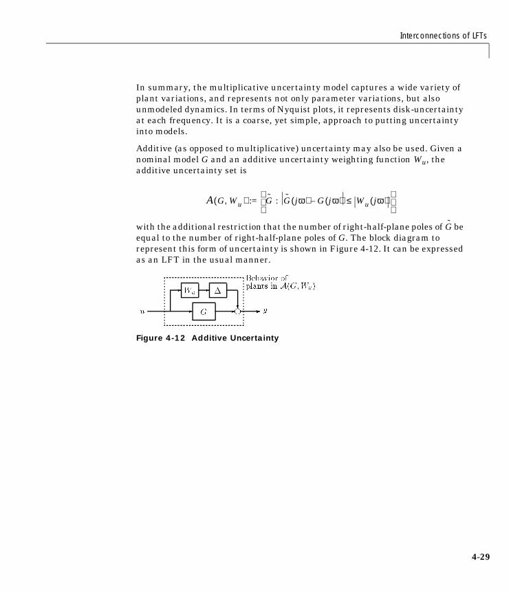
Interconnections of LFTs
In summary, the multiplicative uncertainty model captures a wide variety ofplant variations, and represents not only parameter variations, but alsounmodeled dynamics. In terms of Nyquist plots, it represents disk-uncertaintyat each frequency. It is a coarse, yet simple, approach to putting uncertaintyinto models.
Additive (as opposed to multiplicative) uncertainty may also be used. Given anominal model G and an additive uncertainty weighting function Wu, theadditive uncertainty set is
with the additional restriction that the number of right-half-plane poles of beequal to the number of right-half-plane poles of G. The block diagram torepresent this form of uncertainty is shown in Figure 4-12. It can be expressedas an LFT in the usual manner.
Figure 4-12 Additive Uncertainty
A G Wu,( ) := G : G jω( ) G jω( )– Wu jω( )≤
G
G
Wu
-
- -
?f- - yu
Behavior ofplants in A(G;Wu)
4-29

4 Modeling and Analysis of Uncertain Systems
4-3
Mixed UncertaintyUncertainty may be mixed, including both parametric uncertainty andunmodeled dynamics. For an example, take the uncertain second order systemfrom “Parametric Uncertainty” section, with parametric uncertainty in theparameters m, c, and k and additional high-frequency unmodeled dynamicsusing the multiplicative uncertainty model. The block diagram is
The possible behavior is represented as an LFT
y = FU(Hmix, ∆)u
where the perturbation matrix ∆ has the structure
∆ = diagδm,δc,δk,δ(s)
and Hmix is the five-input, five-output system defined by the following sysiccommands.
systemnames = 'Gmck wu'; sysoutname = 'Hmix'; inputvar = '[parmpertin3 ; unmodpertin ; u]'; input_to_Gmck = '[parmpertin; unmodpertin + u]'; input_to_wu = '[u]'; outputvar = '[Gmck(1:3) ; wu ; Gmck(4)]'; sysic
Gmck
m 0 0
0 c 0
0 0 k
y
6
-
u 6
Wu
6
(s)
?
?
c
? Hmix
0

Analyzing the Effect of LFT Uncertainty
Analyzing the Effect of LFT UncertaintyGiven uncertain models, the structured singular value (µ) can be used toanalyze the robustness of the system to the structured uncertainty that entersin the feedback form.
Using µ to Analyze Robust StabilityAt this point, we have learned how to represent uncertain systems as LFTs onunknown, structured uncertainty matrices. However, there has been nodiscussion on how to analyze the robustness of these uncertain systems. Thisis done with the structured singular value, µ. In this section, we perform ananalysis using the command mu, which computes upper and lower bounds for µ.We concentrate on the mechanics of using the command, and the conclusionsthat you reach with a µ-analysis.
Every µ-analysis consists of the following steps:
1 Recast (using the interconnection program sysic or SIMULINK®) theproblem into the familiar feedback loop diagram of Figure 4-13, where M isa known linear system, and ∆ is a structured perturbation.
Figure 4-13 General Diagram for Robust Stability Analysis
2 Calculate a frequency response of M.
3 Describe the structure of the perturbations ∆.
4 Run the command mu on the frequency response.
5 Plot the bounds obtained from the µ calculation.
M
-
4-31

4 Modeling and Analysis of Uncertain Systems
4-3
Usually M arises by connecting an uncertain system with a feedback controller.Consider the mass/damper/spring system in the “Mixed Uncertainty” section,with both parametric uncertainty and unmodeled dynamics. Suppose that afeedback controller K has been designed to improve the damping, by feedbackfrom y to u, namely u = Ky. Then, the uncertain closed-loop system appears inFigure 4-14.
Figure 4-14 Uncertain Closed-loop System
By grouping Hmix and K together, namely, M := FL(Hmix,K), Figure 4-15 showsthe transformation of Figure 4-14 to Figure 4-13.
Figure 4-15 Transforming to General Form
Hmix
K
-
-
2

Analyzing the Effect of LFT Uncertainty
With M constructed, next we must clearly describe the structure of theuncertain element ∆. The structure of the perturbation matrices must bepassed to the mu command. There are three different aspects to consider abouteach block of the perturbation matrices when specifying the uncertaintystructure:
• The type (real parameter vs. unmodeled dynamics) of the perturbation
• The dimension of the perturbation
• The number of independent locations that the particular uncertainty occurs(that is, does it affect the system in two or more places, as δ1 does in the Gainand Pade parts of the example from the “Parametric Uncertainty” section?)
As for the software, this uncertainty structure information is stored as ann × 2 array (called the block structure array) where n is the number ofdifferent perturbation elements in the uncertainty matrix. Each row of thisblock structure array has information to describe the uncertain block. Inµ-Tools, these conventions are
• A scalar real parameter is denoted [–1 1] (or [–1 0]).
• A repeated (ƒ times) real parameter is denoted [–f 0].
• A 1 × 1 (ie., scalar) unmodeled dynamics perturbation (later referred to ascomplex in the “Structured Singular Value Theory” section), is denoted [1 1]or ([1 0]).
• An r × c (ie., full) unmodeled dynamics block is denoted [r c] See the“HIMAT Robust Performance Design Example” section in Chapter 7 for anexample.
Hence, in the“Parametric Uncertainty” section, the uncertainty set for Gmck isdenoted
deltaset = [–1 1;–1 1;–1 1]; % m/c/k
The uncertainty set for Gproc in the “Parameter Uncertainty in TransferFunctions” section is denoted
deltaset = [–2 0;–1 0]; % Gain/Pade/Lag
The mixed uncertainty example in the “Mixed Uncertainty” section isrepresented as
deltaset = [–1 1;–1 1;–1 1;1 1]; % m/c/k/unmodeled
4-33

4 Modeling and Analysis of Uncertain Systems
4-3
Note that the ordering of the uncertainty elements is (and must be) consistentwith the ordering of the input/output channels of the known systems (Gmck,Gproc, and Hmix).
As a notational convention, once the uncertainty structure has been defined forany given problem, we will use the symbol ∆ to represent all perturbationmatrices with the appropriate structure. For example, in the mixeduncertainty example of the “Mixed Uncertainty” section, we have
Now that the uncertainty structure has been represented, we can compute thesize of perturbations to which the system is robustly stable. We need tocalculate a frequency response of M, and then compute the structured singularvalue (µ) of M with respect to the uncertainty set ∆. At each frequency, thematrix M(jω) is passed to the µ algorithm, and bounds for µ(M(jω)) arecomputed, giving upper and lower bound functions of frequency, which areplotted. The notation for µ will be µ∆(M(jω)), to emphasize the dependency ofthe function not only on M, but also on the uncertainty set ∆.
Suppose the peak (across frequency ω) of the µ∆(M(jω)) is β. This means thatfor all perturbation matrices ∆ with the appropriate structure (ie., any ∆ ∈ ∆),and satisfying , the perturbed system is stable. Moreover,there is a particular perturbation matrix ∆ ∈ ∆ satisfyingthat causes instability. Hence, we think of
as a stability margin with respect to the structured uncertainty set affecting M.
As mentioned, the software does not compute µ exactly, but bounds it fromabove and below by several optimization steps. Hence, the conclusions must becarefully stated in terms of upper and lower bounds. Let βu be the peak (across
∆ :=
δ1 0 0 0
0 δ2 0 0
0 0 δ3 0
0 0 0 δ4
: δ1 R∈ , δ2 R∈ , δ3 R∈ , δ4 s( )
max σ ∆ jω( )[ ] 1β---<ω
max σ ∆ jω( )[ ] 1β---<
ω
1max µ∆ M jω( )( )---------------------------------------------ω
4
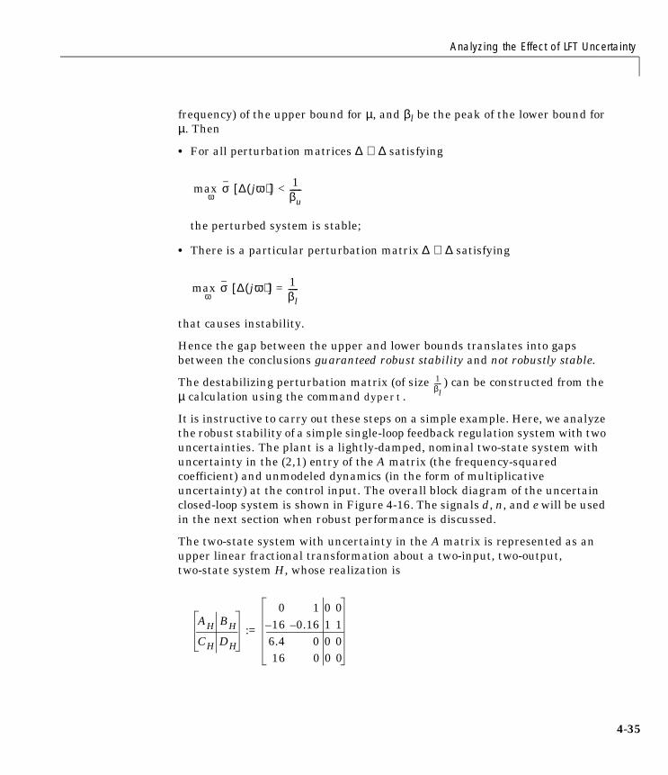
Analyzing the Effect of LFT Uncertainty
frequency) of the upper bound for µ, and βl be the peak of the lower bound forµ. Then
• For all perturbation matrices ∆ ∈ ∆ satisfying
the perturbed system is stable;
• There is a particular perturbation matrix ∆ ∈ ∆ satisfying
that causes instability.
Hence the gap between the upper and lower bounds translates into gapsbetween the conclusions guaranteed robust stability and not robustly stable.
The destabilizing perturbation matrix (of size ) can be constructed from theµ calculation using the command dypert.
It is instructive to carry out these steps on a simple example. Here, we analyzethe robust stability of a simple single-loop feedback regulation system with twouncertainties. The plant is a lightly-damped, nominal two-state system withuncertainty in the (2,1) entry of the A matrix (the frequency-squaredcoefficient) and unmodeled dynamics (in the form of multiplicativeuncertainty) at the control input. The overall block diagram of the uncertainclosed-loop system is shown in Figure 4-16. The signals d, n, and e will be usedin the next section when robust performance is discussed.
The two-state system with uncertainty in the A matrix is represented as anupper linear fractional transformation about a two-input, two-output,two-state system H, whose realization is
max σ ∆ jω( )[ ] < 1βu------
ω
max σ ∆ jω( )[ ] = 1βl-----
ω
1βl-----
AH BH
CH DH
:=
0 1 0 016– 0.16– 1 1
6.4 0 0 016 0 0 0
4-35

4 Modeling and Analysis of Uncertain Systems
4-3
Figure 4-16 Robust Stability/Performance Example
The resulting second order system takes the form
If we assume that δ1 is unknown, but satisfies |δ1| ≤ 1, then we interpret thesecond order system to have 40% uncertainty in the denominator entry of thenatural frequency-squared coefficient.
The plant is also assumed to have unmodeled dynamics at the input. This couldarise from an unmodeled, or unreliable, actuator, for instance. The uncertaintyis assumed to be about 20% at low frequency, rising to 100% at 6 radians/second. We model it using the multiplicative uncertainty model, using afirst-order weight
For this example, the controller is chosen as
Let M(s) in Figure 4-17 denote the closed-loop transfer function matrix fromFigure 4-16, after omitting δ1 and δ2. The dimensions of M are six states, fourinputs and three outputs.
1
5
-n - e+
+-yK
u?
6 de
+
+
Wuz22w2
?e+
+H1
8
e
- 1
w1z1
Uncertain Plant
FU H δ1,( ) 16
s2 0.16s 16 1 0.4δ1+( )+ +---------------------------------------------------------------------=
Wu7s 8.5+s 42+
---------------------=
K 12.56– s2 17.32s 67.28+ +
s3
20.37s2
136.74s 179.46+ + +-------------------------------------------------------------------------------------.=
6

Analyzing the Effect of LFT Uncertainty
Figure 4-17 Closed-loop Interconnection
In the robust stability analysis, we are only concerned about the stability of theperturbed closed-loop system, and in that case, only the transfer function that
the perturbation matrix sees is important. For notational
purposes, drop the s from M(s), and partition M into
(4-4)
where M11 is 2 × 2, and M22 is 1 × 2. The perturbation matrix ∆ enters theproblem as feedback around M11, as shown in Figure 4-18.
Figure 4-18 Example: Robust Stability
Hence, for robust stability calculations we only need the submatrix M11 (forrobust performance calculations, presented in the “Robust Performance”section, we will need the entire matrix M).
The computational steps for analysis are given below:
1 Construct M and check dimensions.
rsexamp; % creates data minfo(M)
M (s)e
z2
z1
n
d
w2
w1
∆ :=δ1 0
0 δ2 s( )
MM11 M12
M21 M22
=
M11
-
4-37
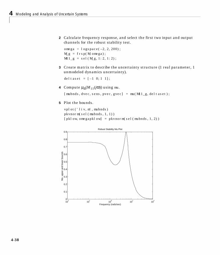
4 Modeling and Analysis of Uncertain Systems
4-3
2 Calculate frequency response, and select the first two input and outputchannels for the robust stability test.
omega = logspace(–2,2,200); M_g = frsp(M,omega); M11_g = sel(M_g,1:2,1:2);
3 Create matrix to describe the uncertainty structure (1 real parameter, 1unmodeled dynamics uncertainty).
deltaset = [–1 0;1 1];
4 Compute µ∆(M11(jω)) using mu.
[mubnds,dvec,sens,pvec,gvec] = mu(M11_g,deltaset);
5 Plot the bounds.
vplot('liv,m',mubnds) pkvnorm(sel(mubnds,1,1)) [pklow,omegapklow] = pkvnorm(sel(mubnds,1,2))
102
101
100
101
102
0
0.1
0.2
0.3
0.4
0.5
0.6
0.7
0.8
0.9Robust Stability Mu Plot
Frequency (rads/sec)
Mu
upp
er a
nd lo
wer
bou
nds
8

Analyzing the Effect of LFT Uncertainty
The peak is about 0.89 (upper and lower bounds are very close in this example)and occurs at ω = 5.4 radians/second. Hence, stability is guaranteed for all
perturbations with appropriate structure, and .
6 Construct the smallest destabilizing perturbation. Check that theperturbation has the appropriate structure and that the size of theperturbation is equal to the reciprocal of the peak of the lower bound.
pert=dypert(pvec,deltaset,mubnds); minfo(pert) seesys(pert) spoles(pert) hinfnorm(sel(pert,1,1)) hinfnorm(sel(pert,2,1)) hinfnorm(sel(pert,1,2)) hinfnorm(sel(pert,2,2)) hinfnorm(pert)
7 Verify that the perturbed system is indeed unstable. Note the location of theperturbed closed-right-half-plane pole and its relationship with the peak ofthe µ-lower bound plot.
pertM = starp(pert,M); spoles(pertM)
max σ ∆ jω( )[ ] < 10.89----------- 1.12≈
ω
4-39

4 Modeling and Analysis of Uncertain Systems
4-4
Using µ to Analyze Robust PerformanceWe have seen how µ can be used to analyze the robust stability of a LFT. In thissection, we use µ to determine the robust performance of a LFT underperturbation.
Assume that the problem has been manipulated (using the program sysic orSimulink) into the familiar feedback loop diagram of Figure 4-19, where M is aknown linear system, ∆ is a structured perturbation from a problem-dependentallowable uncertainty set ∆, and d and e are the generalized disturbance anderror that characterizes the performance objective.
The transformation from a system block diagram to the generic diagram inFigure 4-19 is analogous to the transformation described in this section andFigure 4-15, except that exogenous signals (disturbances and errors) aresimply kept in the diagram.
Figure 4-19 Robust Performance Formulation
Recall from Chapter 3 that the performance of MIMO control systems ischaracterized using H∞ norms. Specifically, we assume that good performanceis equivalent to
where T is some weighted, closed-loop transfer function matrix. In the case ofrobust performance of uncertain systems, we’ll take T to be the uncertaintransfer function from d → e, so T = FU(M,∆).
Clearly, the transfer function from d → e is a function of ∆, through theelements of M, and the linear fractional formula for FU. How large can thetransfer function FU(M,∆) get as ∆ takes on its allowed values? In view of thisquestion, the robust performance condition is defined as: The LFT in Figure
M
-
e d
ω R∈T ∞ := max σ T jω( )( ) 1≤
0

Using µ to Analyze Robust Performance
4-19 is said to achieve robust performance if it is stable for all perturbations ∆∈ ∆ satisfying , and moreover, if ||FU(M,∆)||∞ ≤ 1 for allsuch perturbations.
How can µ be used to assess robust performance? The main idea is very simple— you must first relate the size of a transfer function to a robust stability test.Suppose that T is a given stable system with input dimension nd and outputdimension ne. By the Nyquist and small-gain theorem, we know that ||T||∞ ≤ 1if and only if the feedback loop in Figure 4-20 is stable for every stable ∆F(s) (ofdimension nd × ne) satisfying ||∆F||∞ < 1.
Hence, a transfer function T is small (||T||∞ ≤ β) if and only if T can tolerate allpossible stable feedback perturbations ∆F (with ||∆F||∞ < ) without leading toinstability. In other words, the size of a transfer function could be determinedusing a robust stability test. This ultimately allows us to pose the robustperformance question as a robust stability question.
Figure 4-20 Performance as Robustness
Consider our situation, where T = FU(M,∆). Following the argument presented,we have that ||FU(M,∆)||∞ ≤ 1 for all perturbations ∆ ∈ ∆ satisfying
if and only if the LFT shown in Figure 4-21 is stable for all∆ ∈ ∆ and all stable ∆F satisfying
max σ ∆ jω( )[ ] < 1ω
1β---
T
F
Stable for all kFk1 < 1
-
, T
1 1
max σ ∆ jω( )[ ] < 1ω
max σ ∆ jω( )( ) < 1 andω
max σ ∆F jω( )( ) < 1.ω
4-41

4 Modeling and Analysis of Uncertain Systems
4-4
Figure 4-21 Robust Stability with Augmented Uncertainty
But this is exactly a robust stability problem for M, subjected to perturbationmatrices of the form
Hence, we use robust stability techniques — on a larger problem, computing— to determine bounds on robust performance for our original
problem. Specifically, we use an additional (fictitious) uncertainty element,and determine the robust stability of the extended system, and finally makeconclusions about the robust performance of the original uncertain system,FU(M,∆).
Important: Robust ||⋅||∞ Performance is characterized by introducing afictitious uncertainty block across the disturbance/error channels andcarrying out a Robust Stability Analysis.
In summary, each robust performance µ-analysis consists of the followingsteps:
1 Recast (using the interconnection program sysic or Simulink) the probleminto the familiar feedback loop diagram of Figure 4-19, where M is a knownlinear system, and ∆ is a structured perturbation, and d and e are thegeneralized disturbance and error that characterizes the performanceobjective.
M
F
-
-
∆P∆ 0∆ 0F
=
µ∆PM jω( )( )
2

Using µ to Analyze Robust Performance
2 Calculate a frequency response of M.
3 Describe the structure of the perturbation set ∆.
4 Use the dimensions of the disturbance/error channels to define thefictitiously uncertainty block, and augment this with the actual uncertaintystructure of ∆ to obtain an extended uncertainty set ∆P.
5 Compute µ∆p(M(j,ω)) on the frequency response of M, using the augmenteduncertainty set ∆P (which contains the fictitious full, transfer functionblock).
6 Plot the bounds obtained from the µ calculation.
Suppose the peak of the µ-plot is β. This means that for all perturbationmatrices ∆ ∈ ∆ satisfying , the perturbed system is stableand ||FU(M,∆)||∞ ≤ β. Moreover, there is a particular perturbation ∆ ∈ ∆satisfying that causes either ||FU(M,∆)||∞ = β, or instability.
However, the software does not compute µ exactly, but upper and lowerbounds. Let βu be the peak (across frequency) of the upper bound for µ, and βlbe the peak (across frequency) of the lower bound for µ. Then
• For all perturbation matrices ∆ ∈ ∆ satisfying
the perturbed system is stable and ||FU(M,∆)||∞ ≤ βu.
• There is a particular perturbation matrix ∆ ∈ ∆ satisfying
that causes either ||FU(M,∆)||∞ ≥ βl, or instability.
Hence the gap between the upper and lower bounds leads to gaps in yourinability to precisely determine the robust performance.
There are two exogenous disturbances: a force disturbance d at the input to theplant, and sensor noise n at the measurement. There is a single error, the
max σ ∆ jω( )[ ] < 1β---
ω
max σ ∆ jω( )[ ] = 1β---
ω
max σ ∆ jω( )[ ] < 1βu------ ,
ω
max σ ∆ jω( )[ ] = 1βl-----
ω
4-43

4 Modeling and Analysis of Uncertain Systems
4-4
output of the plant. The (weighted) open-loop transfer functions satisfy 2.6 ≤Ted ≤ 4.0 depending on the value of 1 ≥ δ1 ≥ –1, and of course Ten = 0. Hence theobjective of control is to satisfy
for all allowable perturbations.
In terms of M, we have
T is a 1-output, 2-input system, so the fictitious perturbation block, ∆F, mustbe 2 × 1. Hence, the augmented uncertainty structure has three blocks, andthey are:
• A scalar real parameter;
• A scalar, transfer function uncertainty block;
• A 2 × 1 full transfer function uncertainty block.
deltaset = [–1 0;1 1]; fict_blk = [2 1]; aug_deltaset = [deltaset ; fict_blk];
Now, the nominal value of T is simply FU(M,02×2), which is just M22. Plot themagnitude (versus frequency) of these elements to see the nominal closed-looptransfer function. In the next command, we extract M22 in two different butequivalent manners.
vplot('liv,lm',sel(M_g,3,3:4),starp(zeros(2,2),M_g))
The robust performance µ calculation gives information about how much thesetransfer functions are affected by the linear fractional perturbations δ1and δ2.
max Ted jω( ) 2 Ten jω( ) 2+[ ]
12---
1≤ω
T FU Mδ1 0
0 δ2 s( ),
=
4

Using µ to Analyze Robust Performance
The calculation is carried out on the entire matrix M, using the augmenteduncertainty structure.
[rpbnds,rpdvec,rpsens,rppvec,rpgvec] = mu(M_g,aug_deltaset);vplot('liv,m',rpbnds);
The peak value (of both lower and upper bounds) is about 1.02. This impliesthat robust performance is not quite achieved. In other words, for every
perturbation ∆ = diag [δ1,δ2(s)] satisfying , we are
guaranteed stability and FU(M,∆) ≤ 1.02. Moreover, there is a perturbation ∆ =
diag [δ1,δ2(s)] with such that
||FU(M,∆)||∞ ≈ 1.02 > 1.
102
101
100
101
102
0
0.2
0.4
0.6
0.8
1
1.2Robust Performance Mu Plot
Frequency (rads/sec)
Mu
upp
er a
nd lo
wer
bou
nds
max σ ∆ jω( )[ ] < 11.02-----------
ω
max σ ∆ jω( )[ ] 11.02-----------≈ < 1
ω
4-45
4 Modeling and Analysis of Uncertain Systems
4-4
This can be constructed with dypert, and put into the closed-loop system toverify the degradation of performance.
pert = dypert(rppvec,aug_uncblk,rpbnds,[1;2]); spoles(pert) seesys(pert) hinfnorm(pert) hinfnorm(starp(pert,M)) vplot('liv,lm',vnorm(starp(pert,M_g)))vplot('liv,lm',starp(pert,M_g))
Using µ to Analyze Worst-Case Performance In addition to determining if a system has robust performance to uncertainty,it is useful to get the worst-case perturbation of a given size. For instance,using perturbations of a particular structure ∆, and restricting to those of size≤ α, what is the worst performance possible (as measured in || ⋅ ||∞ norm) andwhat is the perturbation that causes the largest degradation of performance?Precisely given α > 0, the worst-case performance associated with structuredperturbations of size α is defined as
The perturbation matrix which achieves the maximum is denoted ∆bad,α.
The command wcperf assumes that the performance transfer function is anupper loop LFT
FU(M,∆)
so that the uncertainty structure represented by deltaset is closed around theupper loops of M. The corresponding worst-case perturbation can be used inhigh-fidelity time-domain simulations to further understand the effect ofuncertainty. Plotting W(M,α) versus α yields the worst-case performancetradeoff curve, which shows the tradeoff between size of uncertainty andworst-case performance. This can be used to assess the relative merits of twodifferent controllers. The command wcperf computes the performancedegradation curves. The syntax to compute the worst-case perturbation of size
W M ∆ α, ,( ) :=
max σ ∆ jω( )[ ] α≤ω
max FU M ∆,( ) ∞
∆ ∆∈
6

Using µ to Analyze Robust Performance
0.8, and compute the performance degradation curves with at least 10 points isgiven below. The degradation curves are shown in Figure 4-22.
alpha = 0.8; npts = 10; [deltabad,lowbnd,uppbnd] = wcperf(M_g,deltaset,alpha,npts);seesys(deltabad) hinfnorm(deltabad) hinfnorm(starp(deltabad,M)) vplot(lowbnd,uppbnd) grid
Figure 4-22 Worst-Case Performance Degradation Curves
Because µ can only be bounded above and below, the worst-case performancedegradation can also only be bounded. The VARYING matrices lowbnd anduppbnd bound the worst-case performance degradation.
0 0.2 0.4 0.6 0.8 1 1.20
0.5
1
1.5
2
2.5WorstCase Performance Degradation
Size of DELTA
Per
form
ance
Nor
m B
ound
s
4-47

4 Modeling and Analysis of Uncertain Systems
4-4
Summary At this point, you should be well suited to explore the examples involvingµ-analysis, namely the “Analysis of Controllers for an Unstable System”,“MIMO Margins Using µ” and the “Space Shuttle Robustness Analysis”sections in Chapter 7. The rest of this chapter is a theoretical development ofthe properties of µ, and is not necessary reading at this point. Later, as youwork with the µ software, and get comfortable with the interpretation of µ as arobust stability and robust performance measure, we encourage you tocomplete reading this chapter and learn more about this powerful framework.
8

Structured Singular Value Theory
Structured Singular Value TheoryThis section covers a brief description of the mathematical properties of thestructured singular value, µ. The material is mathematical, relying mostly onlinear algebra concepts. Unfortunately, although many of the concepts aresimple, the notation required to state things precisely gets messy andcumbersome. The notation used in this chapter is standard. It is listed in the“Notation” section of Chapter 3.
4-49

4 Modeling and Analysis of Uncertain Systems
4-5
Complex Structured Singular Value
DefinitionsThis section is devoted to defining the structured singular value, a matrixfunction denoted by µ(⋅). We consider matrices M ∈ Cn×n. In the definition ofµ(M), there is an underlying structure ∆, (a prescribed set of block diagonalmatrices) on which everything in the sequel depends. For each problem, thisstructure is in general different; it depends on the uncertainty andperformance objectives of the problem. Defining the structure involvesspecifying three things; the type of each block, the total number of blocks, andtheir dimensions.
There are two types of blocks: repeated scalar and full blocks. Two nonnegativeintegers, S and F, represent the number of repeated scalar blocks and thenumber of full blocks, respectively. To keep tracking of their dimensions, weintroduce positive integers r1,. . . ,rS; m1,. . . ,mF. The ith repeated scalar blockis ri × ri, while the jth full block is mj × mj. With those integers given, we define∆ ⊂ Cn×n as
(4-5)
For consistency among all the dimensions, we must have
Often, we will need norm bounded subsets of ∆, and we introduce the followingnotation
(4-6)
Note that in (4-5) all of the repeated scalar blocks appear first. This is just tokeep the notation as simple as possible, in fact they can come in any order. Also,the full blocks do not have to be square, but restricting them as such saves a
∆ diag δ1Ir1,…,δsIrS
,∆1,…,∆F[ ] : δi C ∆j Cmj mj×
∈,∈
=
ri
i 1=
S
∑ mj
j 1=
F
∑+ n.=
B∆ ∆ ∆∈ : σ ∆( ) 1≤ =
0

Complex Structured Singular Value
great deal in terms of notation. The software will handle nonsquare full blocks,as well as any order to the blocks.
Definition 4.1: For M ∈ Cn×n, µ∆(M) is defined
(4-7)
unless no ∆ ∈ ∆ makes I – M∆ singular, in which case µ∆(M) := 0.
Remark 1: Without loss in generality, the full blocks in the minimal norm ∆can each be chosen to be dyads (rank = 1). To see this, first consider the caseof only 1 full block, ∆ = Cn×n. Suppose that I – M∆ is singular. Then for someunit-norm vector x ∈ CnM∆x = x. Define y := ∆x. It follows that y ≠ 0, and ||y||≤ . Hence, define a new perturbation, as
Obviously, , and , so that is also singular.Hence we have replaced a general perturbation ∆ which satisfies thesingularity condition, with a rank 1 perturbation that is no larger (in thesense), but still satisfies the singularity condition. Repeating this on ablock-by-block basis allows for each full block to be a dyad. The softwarealways carries out this particular construction.
Remark 2: It is instructive to consider a feedback interpretation of µ∆(M)atthis point. Let M ∈ Cn×n be given, and consider the loop shown below.
This picture is meant to represent the loop equations
(4-8)
µ∆ M( ) := 1min σ ∆( ) : ∆ ∆∈ , det I M∆–( ) 0= -------------------------------------------------------------------------------------------------
σ ∆( ) ∆ Cn n×∈
∆ := yx*
σ ∆( ) y σ ∆( )≤= y ∆x= I M∆–
σ .( )
M
-
vu
v ∆u.=
u Mv=
4-51

4 Modeling and Analysis of Uncertain Systems
4-5
As long as I – M∆ is nonsingular, the only solutions u, v to the loop equationsare u = v = 0. However, if I – M∆ is singular, then there are infinitely manysolutions to (4-8), and the norms ||u||, ||v|| of the solutions can be arbitrarilylarge. With an abuse of convention, we call this constant matrix feedbacksystem unstable. Likewise, the term stable will describe the situation when theonly solutions are identically zero. In this context, then, µ∆(M) is a measure ofthe smallest structured ∆ that causes instability of the constant matrixfeedback loop shown above.
An alternative expression for µ∆(M) follows from the definition.
Lemma 4.2:
In view of this lemma, continuity of the function µ : Cn×n → R is apparent. Ingeneral, though, the function µ : Cn×n → R is not a norm, since it doesn’t satisfythe triangle inequality. However, for any α ∈ C, µ(αM) = |α|µ(M), so in somesense, it is related to how big the matrix is in a norm sense.
We can relate µ∆(M) to familiar linear algebra quantities when ∆ is one of twoextreme sets.
• If ∆ = δI : δ ∈ C (S = 1, F = 0, r1 = n), then µ∆(M) = ρ(M), the spectral radiusof M.
Proof: The only ∆’s in ∆ which satisfy the det(I – M∆) = 0 constraint arereciprocals of nonzero eigenvalues of M. The smallest one of these isassociated with the largest (magnitude) eigenvalue, so, µ∆(M) = ρ(M).
• If ∆ = Cn×n (S = 0, F = 1, m1 = n), then
Proof: If , then , so I – M∆ is nonsingular. Applying
equation (4-7) implies . On the other hand, let u and v be unit
vectors satisfying , and define . Then
and I – M∆ is obviously singular. Hence, .
For a general ∆ as in (4-5) we must have
(4-9)
µ∆ M( ) max ρ M∆( )=∆ B∆∈
µ∆M σ M( )=
σ ∆( ) 1σ M( )--------------< σ M∆( ) 1<
µ∆ M( ) σ M( )≤
Mv σ M( )u= ∆ := 1σ M( )--------------vu*
σ ∆( ) 1σ M( )--------------= µ∆ M( ) σ M( )≥
δIn : δ C∈ ∆ Cn n×⊂ ⊂
2

Complex Structured Singular Value
From the definition of µ, and the two special cases above, we conclude that
(4-10)
These bounds alone are not sufficient for our purposes, because the gapbetween ρ and can be arbitrarily large. They are refined by consideringtransformations on M that do not affect µ∆(M), but affect ρ and . To do this,define the following two subsets of Cn×n
(4-11)
(4-12)
Note that for any ∆ ∈ ∆, Q ∈ Q∆, and D ∈ D∆,
(4-13)
(4-14)
ρ M( ) µ∆ M( ) σ M( )≤ ≤
σσ
Q∆ Q ∆∈ : Q*Q In= =
D∆ =diag D1,… DS,d1Im1
,… dF 1–, ImF 1–,ImF
,[ ] :
Di Cri ri×
Di Di* 0 dj R dj 0>,∈,>=,∈
.
Q* Q∆∈ Q∆ ∆∈ ∆Q ∆∈ σ Q∆( ) σ ∆Q( ) σ ∆( )= =
D∆ ∆D.=
4-53

4 Modeling and Analysis of Uncertain Systems
4-5
Consequently,
Theorem 4.3: For all Q ∈ Q∆ and D ∈ D∆
(4-15)
Proof: For all D ∈ D∆ and ∆ ∈ ∆,
det(I – M∆) = det(I – MD–1∆D) = det(I – DMD–1∆)
since D commutes with ∆. Therefore, µ∆(M) = µ∆(DMD–1). Also, for eachQ ∈ Q∆, det(I – M∆) = 0 ⇔ det(I + MQQ*∆) = 0. Since Q*∆ ∈ ∆ and
,we get µ∆(MQ) = µ∆(M) as desired. The argument for QM isthe same.
Therefore, the bounds in (4-10) can be tightened to
(4-16)
where the equality comes from Lemma 2.2. Note that the last element in the Dmatrices in equation (4-12) is normalized to 1 since for any nonzero scalar γ,DMD–1 = (γD)M(γD)–1.
BoundsIn this section we will concentrate on the bounds
The lower bound is always an equality ([Doy]). Unfortunately, the quantityρ(QM) can have multiple local maxima which are not global. Thus local searchcannot be guaranteed to obtain µ, but can only yield a lower bound. The µsoftware actually uses a slightly different formulation of the lower bound as apower algorithm which is reminiscent of power algorithms for eigenvalues andsingular values ([PacD]). While there are open questions about convergence,the algorithm usually works quite well and has proven to be an effectivemethod to compute µ.
µ∆ MQ( ) µ∆ QM( ) µ∆ M( ) µ∆ DMD 1–( )= = =
σ Q*∆( ) σ ∆( )=
max ρ QM( ) max ρ ∆M( )≤ µ∆ M( ) inf σ DMD 1–( )≤=Q Q∆∈ ∆ B∆∈ D D∆∈
max ρ QM( ) µ∆ M( ) inf σ DMD 1–( )≤ ≤Q Q∆∈ D D∆∈
4

Complex Structured Singular Value
The upper bound can be reformulated as a convex optimization problem, so theglobal minimum can, in principle, be found. Unfortunately, the upper bound isnot always equal to µ. For block structures ∆ satisfying 2S + F ≤ 3, the upperbound is always equal to µ∆(M), and for block structures with 2S + F > 3, thereexist matrices for which µ is less than the infimum. This can be summarized inthe following diagram, which shows for which cases the upper bound isguaranteed to be equal to µ.
F
Several of the boxes have connections with standard results.
• S = 0, F = 1 :
• S = 1, F = 0: This is a standard result
in linear algebra. It is also equivalent to fact that Lyapunov stability andexponential stability are equivalent for linear systems.
• S = 0, F = 2: This case was studied by Redheffer ([Red1] and [Red2]).
• S = 1, F = 1: This is equivalent to a standard result on state-spacecomputation of H∞ norms.
• S = 2, F = 0: This is equivalent to the fact that for multidimensional systems(2-d, and higher), exponential stability is not equivalent to Lyapunovstability, [AndAJM], [PacD].
• S = 0, F = 3: For this case, the upper bound is always equal to µ. Thisimportant result is due to Doyle. [Doy]
• S = 0, F ≥ 4: For this case, the upper bound is not always equal to µ. This isimportant, as these are the cases that arise most frequently in applications.Fortunately, the bound seems to be close to µ. The worst known example hasa ratio of µ over the bound of about.85, and most systems are close to 1.
The above bounds are much more than just computational schemes, althoughthat is their primary role in this toolbox. They are also theoretically rich, andcan unify a number of apparently quite different results in linear systemstheory. There are several connections with Lyapunov stability, two of which
0 1 2 3 4
0 yes yes yes no
S 1 yes yes no no no
2 no no no no no
µ∆ M( ) σ M( )=
D D∆∈µ∆ M( ) ρ M( ) inf σ DMD 1–( )= =
4-55

4 Modeling and Analysis of Uncertain Systems
4-5
were hinted at above, but there are further connections between the upperbound scalings and solutions to Lyapunov and Riccati equations. Indeed, manymajor theorems in linear systems theory follow from the upper bounds andsome results for linear fractional transformations (see “Linear FractionalTransformations”). The lower bound can be viewed as a natural generalizationof the maximum modulus theorem [BoyD]. While a complete exposition of theseideas is beyond the scope of this tutorial, some of the more elementary conceptswill be explored in later sections.
For the purposes of this toolbox, the most important use of the upper bound isas a computational scheme when combined with the lower bound. For reliableuse of the µ theory it is essential to have upper and lower bounds. The otherimportant feature of the upper bound is that it can be combined with H∞controller synthesis methods to yield an ad-hoc µ-synthesis method. Note thatthe upper bound, when applied to transfer functions, and maxed acrossfrequencies, is simply a scaled H∞ norm. This is exploited in the µ-synthesistechniques in this toolbox.
Computational Exercise with the mu CommandThe calculation of bounds for the structured singular value (µ) is performedwith the µ-Tools command mu. The input arguments to mu include the matrixon which µ is to be calculated, the block structure associated with the inputmatrix and an optional argument defining the type bound calculations to beperformed. The outputs from mu are the lower and upper bound, scalingmatrices used to achieve the upper bound, a sensitivity measure associatedwith the upper bound calculation and a perturbation matrix ∆ which makesdet(I – M∆) = 0. A more detailed description of the mu can be found in thecommand reference section.
The following exercise uses the command mu to compute upper and lowerbounds for the structured singular value of a given 5 × 5 complex matrix, for avariety of block structures. It is intended to show the dependence of µ∆(M) onthe particular structure ∆. The user can also verify the correctness of thebounds produced by the calculation.
6

Complex Structured Singular Value
The set of commands used are:
Syntax for mu:[bnds,dvec,sens,pvec] = mu(M,deltaset);
Description
is represented by the MATLAB array
mu upper and lower bounds for µ∆(M)
unwrapd unwrap the D scaling matrices associated with upper bound
unwrapp unwrap the perturbation ∆ associated with lower bound
M Matrix to calculate µ of, can be a CONSTANT or VARYINGmatrix.
deltaset block structure information about the set ∆; the number ofperturbation blocks, their sizes and types. For example: theblock structure
∆ :=
δ1 0 0 0
0 δ2 0 0
0 0 δ3 0
0 0 0 δ4
: δi C∈
deltaset
1 11 11 11 1
= .
4-57
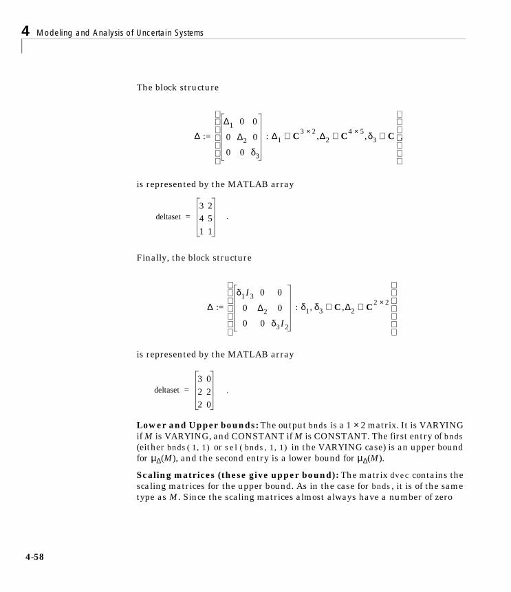
4 Modeling and Analysis of Uncertain Systems
4-5
The block structure
is represented by the MATLAB array
Finally, the block structure
is represented by the MATLAB array
Lower and Upper bounds: The output bnds is a 1 × 2 matrix. It is VARYINGif M is VARYING, and CONSTANT if M is CONSTANT. The first entry of bnds(either bnds(1,1) or sel(bnds,1,1) in the VARYING case) is an upper boundfor µ∆(M), and the second entry is a lower bound for µ∆(M).
Scaling matrices (these give upper bound): The matrix dvec contains thescaling matrices for the upper bound. As in the case for bnds, it is of the sametype as M. Since the scaling matrices almost always have a number of zero
∆ :=
∆1 0 0
0 ∆2 0
0 0 δ3
: ∆1 C3 2× ,∆2 C4 5×∈ ,δ3 C∈∈
,
deltaset3 24 51 1
= .
∆ :=
δ1I3 0 0
0 ∆2 0
0 0 δ3I2
: δ1 δ3, C,∆2 C2 2×∈∈
deltaset3 02 22 0
= .
8

Complex Structured Singular Value
entries, they are stored in dvec as a row vector. They can be unwrapped intothe block diagonal form using unwrapd.
[Dl,Dr] = unwrapd(dvec,deltaset);
For the most part, these two matrices are the same, in fact, if the blockstructure deltaset has no nonsquare full blocks, then Dl = Dr. In any event,the following are always true:
and .
Sensitivity (used in µ-synthesis): a sensitivity measure of the maximumsingular value of with respect to the values in Dl (and Dr). It iscalculated in an ad-hoc manner, and is mainly used when fitting frequencyvarying D’s with rational functions via the routine fitsys. We will not makeuse of it in this example.
Perturbation (gives lower bound): The matrix pvec contains theperturbation matrix ∆ which makes I – M∆ singular. This perturbationcorresponds to the lower bound in bnds. It is of the same type as M. Since thestructured set usually contains many zero elements, the perturbation matrix ∆is stored efficiently in pvec as a row vector. It can be unwrapped into the blockdiagonal form using unwrapp.
delta = unwrapp(pvec,deltaset);
Note that is equal to the reciprocal of the lower bound (in bnds), and
Try this on some examples:
simplemu;
This creates a 5 × 5 matrix, M, and the different block structures, deltaseta, deltasetb,...,deltaseti.
Dl Dl* 0>= ,Dr Dr
* 0 Dr∆ ∆=,>= Dl ∆∀ ∆∈
µ∆ M( ) σ DlMDr1–( )≤
DlMDr1–
σ ∆( )
∆ ∆∈det I M∆–( ) = 0
4-59

4 Modeling and Analysis of Uncertain Systems
4-6
Consider the block structure defined by the array deltasete. Run the mucommand, and unwrap the ds and the perturbation.
[bnds,dvec,sens,pvec] = mu(M,deltasete); [Dl,Dr] = unwrapd(dvec,deltasete); delta = unwrapp(pvec,deltasete);
Verify that
• ∆ ∈ ∆; print out the matrix delta, and check that its structure correspondsto that given by the array deltasete
• Compare the norm of the matrix delta with the lower bound from bnds
bnds norm(delta);
• Note that the should equal the inverse of the lower bound(1 bnds(1,2)).
• Verify that det(I5 – M∆) = 0det(eye(5)-M*delta)
or
eig(M*delta) % should have an eigenvalue at 1
• Look at the scaling matrices Dl and Dr. Note that Dr∆ = ∆Dl for all ∆ ∈ ∆.Check that the upper bound in bnds comes from these.
bnds(1,1) norm(Dl*M/Dr)
Try the other examples, and verify the consistency of all aspects of the results.
σ ∆( )
0

Mixed Real/Complex Structured Singular Value
Mixed Real/Complex Structured Singular ValueUp until this point, this chapter has dealt only with complex-valuedperturbation sets, as in equation (4-5), and the complex structured singularvalue to assess stability and performance degradation under these types ofperturbations. In specific instances, we have seen that it may be more naturalto model some of the uncertainty with real perturbations, for instance when thereal coefficients of a linear differential equation are uncertain. While it ispossible to simply treat these perturbations as complex and proceed with thecomplex-µ analysis, the results can be expected to be conservative. Hence,researchers have developed algorithms for robustness tests with both real andcomplex perturbation blocks. The command mu also works for these extremelyuseful calculations.
Hence, there are three different types of uncertainty blocks allowed in the musoftware:
• Repeated scalar real blocks
• Repeated scalar complex blocks
• Full complex blocks
The general structured singular value theory also includes full real blocks, butthese are difficult to motivate from the physics of real problems, andconvenient upper and lower bounds for structures with these types of blocksare not well developed. This is an ongoing area of research, and later versionsof µ-Tools may support these types of blocks.
The theory for a mixed real/complex upper bound is more complicated todescribe than the upper bound theory for complex µ. In addition to D matrices,which exploit the block diagonal structure of the perturbation, there are Gmatrices, which exploit the real structure of the perturbations. For illustrativepurposes, consider a specific block structure. Suppose that
∆ :=
δ1I2 2× 0 0
0 δ2I4 4× 0
0 0 ∆3
: δ1 R ,δ2 C∈ ,∆3 C3 3×∈∈
4-61

4 Modeling and Analysis of Uncertain Systems
4-6
In mu, this is denoted by
deltaset = [–2 0;4 0;3 3];
A zero (0) in the second column signifies a repeated scalar block (as before). Thenegative sign (–) indicates a real block.
Associated with ∆, define the sets
and
If there is a β > 0, D ∈ D∆ and G ∈ G∆ such that
(4-17)
then
µ∆(M) ≤ β
This bound, [YouND1], is a derivative of an earlier bound in [FanTD]. Thesmallest β < 0 for which D and G matrices exist which satisfy this constraint iswhat µ-Tools calls the mixed µ upper bound for M. Using manipulations thatare now standard in robust control theory, the computation of the best such βis reformulated into an Affine Matrix Inequality (AMI) and solved with specialpurpose convex programming techniques. For perturbation sets with multiple
D∆ =
D1 0 0
0 D2 0
0 0 d3I3 3×
: D1 C2 2×∈ ,det D1( ) 0≠
D2 C4 4×∈ ,det D2( ) 0,d3 C∈ ,d3 0≠≠
G∆ =
diag gi[ ]i 1 2,=0 0
0 04 4× 0
0 0 02 2×
: gi R∈
σ I G2+( )
14---– 1
β---DMD 1– jG–
I G2+( )
14---–
1≤
2

Mixed Real/Complex Structured Singular Value
blocks, the general structure of the sets D∆ and G∆ remains the same, with onescaling block for each uncertainty block.
In mu, only the complex full blocks can be nonsquare. This causes the Dscaling on the left of M to be slightly different from the D scaling on the right.The single d variable associated with the full block is repeated a certainnumber of times on the left, and a different number of times on the right,leading to nonsquare D scaling matrices (the Dl and Dr that we have alreadyseen). Of course, the G scaling comes in different sizes too. Note that for anycomplex full blocks, the associated blocks of G are zeros, since G is onlynonzero in the blocks associated with the real uncertainties. However, thedimension of the zero blocks of G must line up with the correct rows/columnsof M. Hence, in equation (4-17), there are three different Gs, all havingexactly the same nonzero elements, but different sizes of zero blocksassociated with any nonsquare full blocks. The different Gs are denoted Gl,Gm, and Gr. The sufficient condition for the µ∆(M) < β is rewritten as
(4-18)
The lower bound generated in mu comes from a power iteration which findsmatrices ∆ ∈ ∆ that make I – M∆ singular. The power iteration for mu is ageneralization of the power iteration used in earliest versions of µ-Tools. Thegeneralization is described in detail in [YouD].
The combination of upper and lower bounds makes the mu software unique. Theupper bounds give a guarantee on the worst-case performance degradationthat can occur under perturbation. The lower bounds actually exhibit aperturbation that causes significant performance degradation. Thisperturbation can then be used in time-domain simulations to betterunderstand its effect.
σ I Gl2
+( )14---– 1
β---DlMDr
1– jGm– I Gr
2+( )
14---–
1.≤
4-63

4 Modeling and Analysis of Uncertain Systems
4-6
Specifics About Using the mu Command with Mixed PerturbationsThe syntax of mu and muunwrap are
[bnds,dvec,sens,pvec,gvec] = mu(M,deltaset,options);[dl,dr,gl,gm,gr] = muunwrap(dvec,gvec,deltaset); [delta] = muunwrap(pvec,deltaset);
Their purposes are:
Other functions associated with mu (such as unwrapd and unwrapp, which havebeen illustrated already) are detailed in Chapter 8, “Reference” under mu.
Computational Exercise with the mu Command — Mixed PerturbationsThe input argument deltaset is as before, but real repeated scalar blocks arespecified with a negative integer rather than a positive integer. For example,deltaset = [–3 0; 2 3] is similar to deltaset = [3 0; 2 3] except that the3 × 3 repeated block is treated as real rather than complex. Also note thatredefining deltaset = abs(deltaset) always gives the complex version of amixed µ problem.
For instance, the block structure
is represented by the array
deltaset = [1 1;1 1;–1 0;–1 0];
mu general mixed µ computation
muunwrap extract block-diagonal scalings D and G from row vectors, andextract from row vector the smallest perturbation ∆ whichcauses singularity.
∆ :=
δ1 0 0 0
0 δ2 0 0
0 0 δ3 0
0 0 0 δ4
: δi C,i 1 2 δj, ,= R∈ ,j 3 4.,=∈
4

Mixed Real/Complex Structured Singular Value
The block structure
is represented by the array
deltaset = [3 2;4 5;–3 0];
Finally, the block structure
is represented by the array
deltaset = [3 0;2 2;–2 0];
The correctness of the upper bound can easily be checked with the inequalityin equation (4-18). The correctness of the lower bound can be verified bycalculating the perturbation, ∆, that mu returns, verifying its block structureand norm, checking that the matrix M∆ has an eigenvalue exactly at 1 (whichis equivalent to I – M∆ being singular).
Try some examples on a constant 5 × 5 matrix.
simprmu
This loads a 5 × 5 complex matrix, M, and different block structuresdeltaseta, deltasetb,...,deltaseti. Consider the block structure ∆defined by deltasete, Run the mu command, and unwrap the D, G, andperturbation matrices.
[bnds,dvec,sens,pvec,gvec] = mu(M,deltasete); [dl,dr,gl,gm,gr] = muunwrap(dvec,gvec,deltasete); [delta] = muunwrap(pvec,deltasete);
∆ diag [∆1 ∆2 δ3I3 3× ] : ∆1 C3 2×,∆2 C4 5×∈ ,δ3 R∈∈
,=
∆ :=
δ1I3 3× 0 0
0 ∆2 0
0 0 δ3I2 2×
: δ1 C,δ3 R∈ ,∆2 C2 2×∈∈
4-65

4 Modeling and Analysis of Uncertain Systems
4-6
Verify that
• ∆ ∈ ∆; print out delta, and check that its block structure corresponds to thatgiven by deltasete
deltasete delta
• Compare the lower bound from µ with the norm of ∆[bnds(1,2) 1/norm(delta)]
• Verify that det(I5 – M∆) = 0eig(M*delta)
• Verify the upper bound by checking the structure of dl, dr, gl, gm, and gr,and the inequality in equation (4-18)
deltasete dl dr gl gm gr oobdmdimjg = 1/bnds(1,1)*dl*mat/dr – sqrt(–1)*gm; gscl_l = inv(sqrtm(sqrtm(eye(5) + gl*gl)))); gscl_r = inv(sqrtm(sqrtm((eye(5) + gr*gr))));norm(gscl_l*oobdmdimjg*gscl_r)
Try the other block structures, and verify the consistency of all aspects of thebounds, scaling matrices, and perturbations.
6

Linear Fractional Transformations
Linear Fractional TransformationsUsing only the definition of µ, some simple theorems about a class of generalmatrix transformations called linear fractional transformations can be proven.To introduce these, consider a complex matrix M partitioned as
(4-19)
and suppose there is a defined block structure ∆2 which is compatible in sizewith M22 (for any ∆2 ∈ ∆2, M22∆2 is square). For ∆2 ∈ ∆2, consider the followingloop equations,
(4-20)
This set of equations (4-20) is called well posed if for any vector d, there existunique vectors w, z, and e satisfying the loop equations. It is easy to see thatthe set of equations is well posed if and only if the inverse of I – M22∆2 exists.If not, then depending on d and M, there is either no solution to the loopequations, or there are an infinite number of solutions. When the inverse doesindeed exist, the vectors e and d must satisfy e = FL(M,∆2)d, where
(4-21)
FL(M,∆2) is called a Linear Fractional Transformation on M by ∆2, and in afeedback diagram appears as:
MM11 M12
M21 M22
=
e M11d M12w+=
w ∆2z=z M21d M22w+=
FL M ∆2,( ) M11 M12∆2 I( M22∆2 ) 1– M21–+=
e
M
z
-
d
w
2
4-67

4 Modeling and Analysis of Uncertain Systems
4-6
The subscript L on FL pertains to the lower loop of M and is closed by ∆2. Ananalogous formula describes FU(M,∆1), which is the resulting matrix obtainedby closing the upper loop of M with a matrix ∆1 ∈ ∆1.
In this formulation, the matrix M11 is assumed to be something nominal, and ∆2 ∈ B2 := is viewed as a norm-bounded perturbationfrom an allowable perturbation class, ∆2. The matrices M12, M21, and M22 andthe formula FL reflect prior knowledge on how the unknown perturbationaffects the nominal map, M11. This type of uncertainty, called linear fractional,is natural for many control problems, and encompasses many other specialcases considered by researchers.
The constant matrix problem to solve is:
• determine whether the LFT is well posed for all ∆2 ∈ B2, and,
• if so, then determine how large FL(M,∆2) can get for this norm-bounded setof perturbations.
The next section has three simple theorems which answer this problem.
Well Posedness and Performance for Constant LFTsLet M be a complex matrix partitioned as
(4-22)
and suppose there are two defined block structures, ∆1 and ∆2, which arecompatible in size with M11 and M22 respectively. Define a third structure ∆ as
(4-23)
Now there are three structures with which we may compute µ. The notation weuse to keep track of this is as follows: µ1(⋅) is with respect to ∆1, µ2(⋅) is withrespect to ∆2, : µ∆ (⋅) is with respect to ∆. In view of this, µ1(M11), µ2(M22), andµ∆(M) all make sense, though for instance, µ1(M) does not. Again, define thenorm-bounded perturbation sets as
∆2 ∆2 : σ ∆2( )∈ 1≤
MM11 M12
M21 M22
=
∆∆1 0
0 ∆2
: ∆1 ∆1 ∆2 ∆2∈,∈
= .
8

Linear Fractional Transformations
Let ∆2 ∈ ∆2. The linear fractional transformation, FL(M,∆2) is well posed ifI - M22∆2 is invertible, and in that case is defined as
(4-24)
The first theorem is nothing more than restating the definition of µ.
Theorem 4.4: The linear fractional transformation FL(M,∆2) is well posed forall ∆2 ∈ B2 if and only if µ2(M22) < 1.
As the perturbation ∆2 deviates from zero, the matrix FL(M,∆2) deviates fromM11. The range of values that µ1(FL(M,∆2))takes on is intimately related toµ∆(M), as follows:
Theorem 4.5 [Main Loop Theorem]: The following are equivalent:
1 µ∆(M) <1
2 µ2(M22) < 1, and
3 µ1(M11) < 1, and
Proof: The proof is based on Schur formulae for determinants of blockpartitioned matrices, and can be found in [PacD]. The basic idea is simple, andwe present the proof showing 3 → 1.
Bi ∆i ∆i : σ ∆i( )∈ 1≤ =: .
FL M ∆2,( ) M11 M12∆2 I( M22∆2 ) 1– M21–+=
max µ1 FL M ∆2,( )( ) 1<∆2 B2∈
max µ2 FU M ∆1,( )( ) 1<∆1 B1∈
4-69
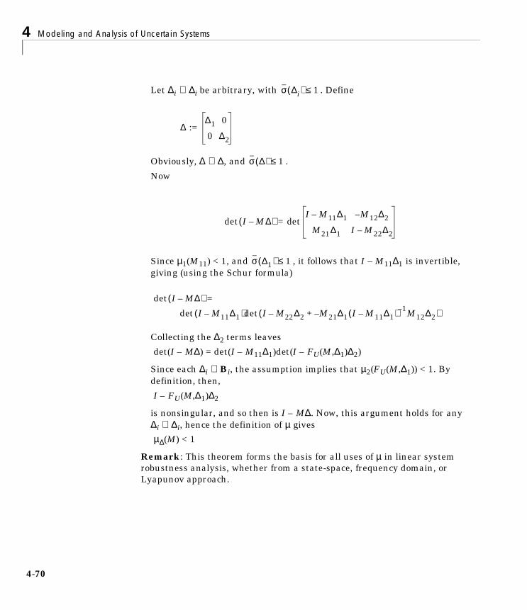
4 Modeling and Analysis of Uncertain Systems
4-7
Let ∆i ∈ ∆i be arbitrary, with . Define
Obviously, ∆ ∈ ∆, and .
Now
Since µ1(M11) < 1, and , it follows that I – M11∆1 is invertible,giving (using the Schur formula)
Collecting the ∆2 terms leaves
det(I – M∆) = det(I – M11∆1)det(I – FU(M,∆1)∆2)
Since each ∆i ∈ Bi, the assumption implies that µ2(FU(M,∆1)) < 1. Bydefinition, then,
I – FU(M,∆1)∆2
is nonsingular, and so then is I – M∆. Now, this argument holds for any∆i ∈ ∆i, hence the definition of µ gives
µ∆(M) < 1
Remark: This theorem forms the basis for all uses of µ in linear systemrobustness analysis, whether from a state-space, frequency domain, orLyapunov approach.
σ ∆i( ) 1≤
∆ :=∆1 0
0 ∆2
σ ∆( ) 1≤
det I M∆–( ) = detI M11∆1– M– 12∆2
M21∆1 I M– 22∆2
σ ∆1( ) 1≤
det I M∆–( ) =
det I M11∆1–( )det I M22∆2– M21∆1– I M11∆1–( ) 1–+ M12∆2( )
0

Frequency Domain µ Review
Frequency Domain µ Review Since the frequency domain µ tests play a key role in robustness analysis, wesummarize in this section the computational procedure and its subsequentinterpretations. These involve not only constant, complex structuredperturbations, but also linear, time-invariant, dynamical perturbations(unmodeled dynamics) as well.
Robust StabilityThe most well-known use of µ as a robustness analysis tool is in the frequencydomain. Suppose M(s) is a stable, multi-input, multi-output transfer functionof a linear system, M. For clarity, assume M has nz inputs and nw outputs. Let∆ be a block structure, as in equation (4-5), and assume that the dimensions aresuch that . We want to consider feedback perturbations to M whichare themselves dynamical systems, with the block-diagonal structure of the set∆.
In this section, we outline the proofs for the situation where the perturbationsare assumed to be stable. This is not a restriction with parametric realuncertainty, as constant parameters are clearly stable. However, when using amultiplicative or additive unmodeled dynamics perturbation to modeluncertainty in an unstable component (see the example in the “UnmodeledDynamics” section), it is useful to allow unstable perturbations, with therestriction that the number of right-half-plane poles of the component remainsconstant. An alternate approach is to allow a block of the perturbation matrixto be an unstable transfer function. However, we restrict it to only take onvalues that preserve the number of right-half-plane poles of the perturbedcomponent with which it is associated. In this case, the theorems we state arestill correct, though the proofs must be modified. In fact, even moresophisticated assumptions about the perturbed systems can be made, includingstructured coprime factor uncertainty and gap metric uncertainty, but theseare beyond the scope of this tutorial.
Let S denote the set of real-rational, proper (no poles at s = ∞), stable, transfermatrices. Associated with any block structure ∆, let S∆ denote the set of allblock diagonal, stable rational transfer functions, with block structure like ∆.
∆ Cnz nw×⊂
S∆ := ∆ S : ∆ so( ) ∆∈ ∈ for all so C+∈
4-71
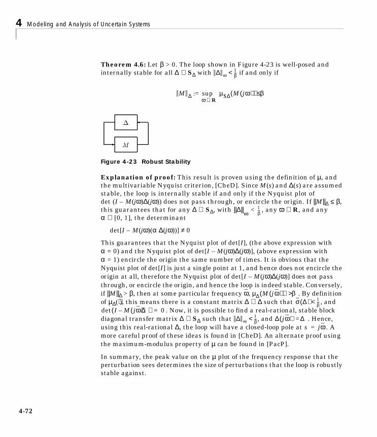
4 Modeling and Analysis of Uncertain Systems
4-7
Theorem 4.6: Let β > 0. The loop shown in Figure 4-23 is well-posed andinternally stable for all ∆ ∈ S∆ with if and only if
Figure 4-23 Robust Stability
Explanation of proof: This result is proven using the definition of µ, andthe multivariable Nyquist criterion, [CheD]. Since M(s) and ∆(s) are assumedstable, the loop is internally stable if and only if the Nyquist plot ofdet (I – M(jω)∆(jω)) does not pass through, or encircle the origin. If ||M||∆ ≤ β,this guarantees that for any ∆ ∈ S∆, with ||∆||∞ < , any ω ∈ R, and anyα ∈ [0, 1], the determinant
det[I – M(jω)(α ∆(jω))] ≠ 0
This guarantees that the Nyquist plot of det[I], (the above expression withα = 0) and the Nyquist plot of det[I – M(jω)∆(jω)], (above expression withα = 1) encircle the origin the same number of times. It is obvious that theNyquist plot of det[I] is just a single point at 1, and hence does not encircle theorigin at all, therefore the Nyquist plot of det[I – M(jω)∆(jω)] does not passthrough, or encircle the origin, and hence the loop is indeed stable. Conversely,if ||M||∆ > β, then at some particular frequency . By definitionof µ∆(⋅), this means there is a constant matrix ∆ ∈ ∆ such that , and
. Now, it is possible to find a real-rational, stable blockdiagonal transfer matrix ∆ ∈ S∆ such that , and . Hence,using this real-rational ∆, the loop will have a closed-loop pole at . Amore careful proof of these ideas is found in [CheD]. An alternate proof usingthe maximum-modulus property of µ can be found in [PacP].
In summary, the peak value on the µ plot of the frequency response that theperturbation sees determines the size of perturbations that the loop is robustlystable against.
∆ ∞1β---<
M ∆ sup µ$∆ M jω( )( ) β≤=ω R∈
:
M
-
1β---
ω µ∆ M jω( )( ) β>,σ ∆( ) 1
β---<
det I M jω( )∆–( ) 0=∆ ∞
1β---< ∆ jω( ) ∆=
s jω=
2
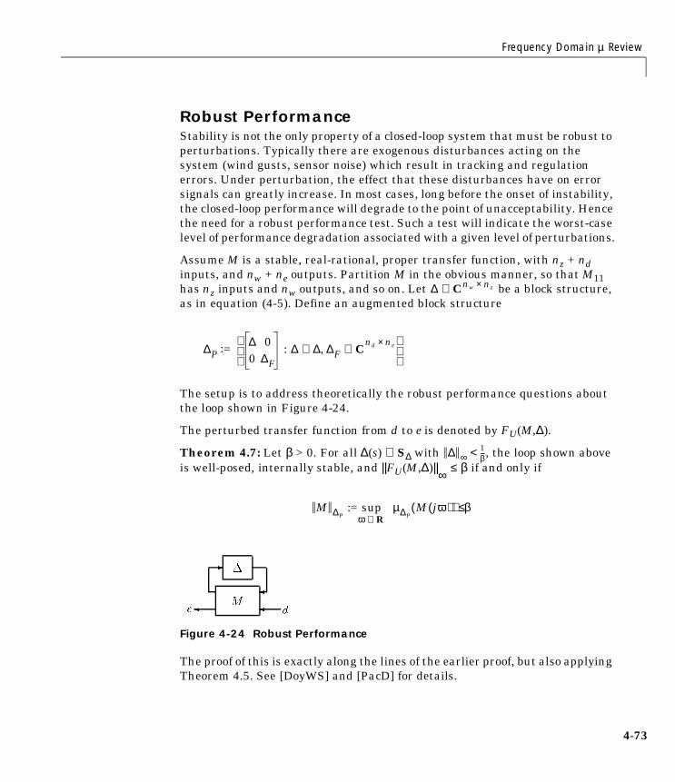
Frequency Domain µ Review
Robust PerformanceStability is not the only property of a closed-loop system that must be robust toperturbations. Typically there are exogenous disturbances acting on thesystem (wind gusts, sensor noise) which result in tracking and regulationerrors. Under perturbation, the effect that these disturbances have on errorsignals can greatly increase. In most cases, long before the onset of instability,the closed-loop performance will degrade to the point of unacceptability. Hencethe need for a robust performance test. Such a test will indicate the worst-caselevel of performance degradation associated with a given level of perturbations.
Assume M is a stable, real-rational, proper transfer function, with nz + ndinputs, and nw + ne outputs. Partition M in the obvious manner, so that M11has nz inputs and nw outputs, and so on. Let be a block structure,as in equation (4-5). Define an augmented block structure
The setup is to address theoretically the robust performance questions aboutthe loop shown in Figure 4-24.
The perturbed transfer function from d to e is denoted by FU(M,∆).
Theorem 4.7: Let β > 0. For all ∆(s) ∈ S∆ with , the loop shown aboveis well-posed, internally stable, and ||FU(M,∆)||∞ ≤ β if and only if
Figure 4-24 Robust Performance
The proof of this is exactly along the lines of the earlier proof, but also applyingTheorem 4.5. See [DoyWS] and [PacD] for details.
∆ Cnw nz×⊂
∆P∆ 00 ∆F
: ∆ ∆ ∆F Cnd ne×
∈,∈
=:
∆ ∞1β---<
M ∆P:= sup µ∆P
M jω( )( ) β≤ω R∈
M
-
e d
4-73

4 Modeling and Analysis of Uncertain Systems
4-7
Real vs. Complex ParametersThere are many approaches to model real, uncertain parameters. Suppose thata coefficient c, in a particular system, is assumed to be constant, but unknown,and the value of c is modeled to lie in an interval, say,
c ∈ [0.8 1.6]
This can be modeled effectively with a real perturbation,
c ∈ 1.2 + (0.4)δ : δ ∈ R, |δ| ≤ 1
Clearly, this set captures the uncertainty in the coefficient c. What is thecorrect interpretation of the uncertain set model if δ is taken as complex,
c ∈ 1.2 + (0.4)δ : δ ∈ C, |δ| ≤ 1 ?
In a linear, time-invariant system, robustness to this constant, complexuncertain parameter c is mathematically equivalent to robustness to all stable,linear, time-invariant transfer functions, , whose Nyquist plots lie in thedisk shown in Figure 4-25.
Figure 4-25 Complex Disc Covering Real Interval: Restriction of the Nyquist Plot of
Using complex parameters, the uncertain model for c represents a stable linearsystem whose characteristics are similar to an uncertain real gain, but deviatein a manner quantified by the disc-shaped constraint on its frequency response.In general, using disks instead of intervals leads to more conservativerobustness properties. With mu, it is easy and fast to explore the differences inthe robustness properties as the uncertainty model changes.
c s( )
6
-
C
Re
Im
0:8
0:4
0:4
0:8
0:8 0:4 0:4 0:8 1:2 1:6 2:0&%'$
c
4

Real vs. Complex Parameters
Block Structures with All Real Blocks The function µ is not necessarily a continuous function when all of theperturbation blocks are real. This mathematical fact is pointed out in[BarKST], and an example is given where the robustness margin to realparameter uncertainty changes abruptly for infinitesimal changes in theproblem data. Also, in the [BarKST] example, the structured singular value ofthe frequency response exhibits discontinuities across frequency.
What is the significance of these issues on mu? The discontinuities can causeproblems in the convergence of the lower bound power algorithm. For problemswith purely real uncertainty, the lower bound algorithm may converge to avalue which is significantly lower than µ itself, or may not even converge at all.This could be a serious problem, but usually it is not, because almost allproblems have a full complex block associated with a robust performancespecification. It turns out that if a µ problem has a complex block that counts,then the function µ will be continuous at the problem data.
Sometimes, though, a robust stability calculation for an uncertain system withonly real uncertainties is needed. Consider the robust stability problemrepresented in Figure 4-26.
Figure 4-26 Robust Stability with Real Uncertainty
While the upper bound from mu will be effective, the lower bound potentiallywill have convergence problems, yielding little information in terms of badperturbations. A fix, which has both engineering and mathematicaljustification, is available.
R
M
-
4-75

4 Modeling and Analysis of Uncertain Systems
4-7
In µ-Tools vernacular, let M be the VARYING matrix (usually a frequencyresponse) of which µ is to be computed. Let blkrs_R be the real block structure,that is compatible in dimension with M. Recall that abs(blkrs_R) is exactly thesame block structure as blkrs_R, but consists of complex blocks. Define:
pdim = ynum(M); %only real blocks --> square alpha = 0.1; fixl = [eye(pdim) ; alpha*eye(pdim)]; fixr = fixl'; % duplicate complex blocks below reals blkrs_RC = [blkrs_R ; abs(blkrs_R)]; Mmix = mmult(fixl,M,fixr); [bnd_RC,rowd_RC,sens,rowp_RC] = mu(Mmix,blkrs_RC);
What does all of this mean? The block structure has been expanded (to twicethe original size) by including complex blocks which are exactly the samedimension as the original real blocks. The matrix has been expanded (to twicethe original size) by the multiplication on the left and right. The scale factorsof α = 0.1 imply that the input/output channels, which the complex uncertaintyaffects, are each scaled down by a factor of 10, giving an overall scaling of thecomplex blocks of 0.01. The µ calculation determines upper and lower boundsfor robust stability in the uncertain system shown in Figure 4-27.
Figure 4-27 Replacing Real Uncertainty with Real+Complex Uncertainty
In this process, each real parameter δR has been replaced by a realparameter plus a smaller complex parameter (α2δC). Rather than computingrobustness margins to purely real parameters, the modified problemdetermines the robust stability characteristics of the system with respect to
C
R
M
-
6 c
-
?
R + 2C
M
-
6

Real vs. Complex Parameters
predominantly real uncertainties, though each uncertainty is allowed tohave a very small complex part. This slight variation in the uncertaintymodel is easy to accept in engineering problems, since models of uncertaintyare rarely fixed, and small amounts of phase in coefficients of physicalmodels usually can be explained by some underlying dynamics that havebeen ignored. It can also be proven that as the parameter α converges to 0,the calculated robustness margin, which is a function of α, converges to therobustness margin associated with just the original real parameters.
In summary, the modified problem contains both real and complex uncertainty;consequently,
• µ with respect to this structure has guaranteed continuity properties.
• The lower bound from mu generally has better convergence behavior.
Moreover, although the modified problem is not equivalent to the originalproblem, it has relevant engineering interpretation and provable convergenceproperties as the complex weighting α goes to 0.
As an example of this, consider the 9 × 9 transfer function M(s), with a robuststability uncertainty block structure of
∆R := diag[δi]i=1,. . .,9 : δi ∈ R,
from the “Space Shuttle Robustness Analysis” section in Chapter 7. Using mu,calculate the robust stability of the system in Figure 4-26, and for α = 0.1, 0.2,0.3 in Figure 4-27.
4-77

4 Modeling and Analysis of Uncertain Systems
4-7
load shut_rs minfo(clp_muRS) blkrs_R = [–1 0;–1 0;–1 0;–1 0;–1 0;–1 0;–1 0;–1 0;–1 0];clp_muRSg = frsp(clp_muRS,logspace(–2,2,40)); fix1 = [eye(9) ; 0.1*eye(9)]; fix2 = [eye(9) ; 0.2*eye(9)]; fix3 = [eye(9) ; 0.3*eye(9)]; blk_RC = [blkrs_R ; abs(blkrs_R)]; m1 = mmult(fix1,clp_muRSg,fix1); m2 = mmult(fix2,clp_muRSg,fix2); m3 = mmult(fix3,clp_muRSg,fix3); [rbnd,rp] = mu(clp_muRSg,blkrs_R); [bnd1,rd1,s1,rp1] = mu(m1,blk_RC); [bnd2,rd2,s2,rp2] = mu(m2,blk_RC); [bnd3,rd3,s3,rp3] = mu(m3,blk_RC); allbnds = abv(rbnd,bnd1,bnd2,bnd3); vplot('liv,d',sel(allbnds,':',1)) title('UPPER BOUNDS: 0%, 1%, 4%, 9% COMPLEX') xlabel('FREQUENCY, RAD/SEC') ylabel('UPPER BOUND') vplot('liv,d',sel(allbnds,':',2)) title('LOWER BOUNDS: 0%, 1%, 4%, 9% COMPLEX') xlabel('FREQUENCY, RAD/SEC') ylabel('LOWER BOUND')
8
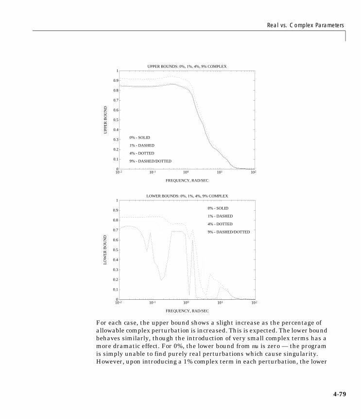
Real vs. Complex Parameters
For each case, the upper bound shows a slight increase as the percentage ofallowable complex perturbation is increased. This is expected. The lower boundbehaves similarly, though the introduction of very small complex terms has amore dramatic effect. For 0%, the lower bound from mu is zero — the programis simply unable to find purely real perturbations which cause singularity.However, upon introducing a 1% complex term in each perturbation, the lower
0
0.1
0.2
0.3
0.4
0.5
0.6
0.7
0.8
0.9
1
10-2 10-1 100 101 102
UPPER BOUNDS: 0%, 1%, 4%, 9% COMPLEX
FREQUENCY, RAD/SEC
UP
PE
R B
OU
ND
0% - SOLID
1% - DASHED
4% - DOTTED
9% - DASHED/DOTTED
0
0.1
0.2
0.3
0.4
0.5
0.6
0.7
0.8
0.9
1
10-2 10-1 100 101 102
LOWER BOUNDS: 0%, 1%, 4%, 9% COMPLEX
FREQUENCY, RAD/SEC
LOW
ER
BO
UN
D
0% - SOLID
1% - DASHED
4% - DOTTED
9% - DASHED/DOTTED
4-79

4 Modeling and Analysis of Uncertain Systems
4-8
bound jumps up to 0.76, indicating mu has found a diagonal perturbationcausing singularity, with each term of the perturbation having the form δR +0.01δC, δR ∈ R, δC ∈ C, and
Using unwrapp, this perturbation can be constructed. For larger values ofcomplex contribution, the lower bound is even better behaved, and more closelymatches up with the corresponding upper bound. Of course, the relevance ofthese nonreal perturbations on the actual robust stability properties must beassessed through careful engineering judgement and considerations.
[PacP] contains a more detailed discussion of the continuity properties of mixedµ, and the general relationship between the robustness bound in Figure 4-26and Figure 4-27.
Finally, in defense of mu— usually, robustness problems involve a performanceobjective, beyond robust stability. This performance objective leads to a fullcomplex block in the uncertainty block structure (when calculating robustperformance tests, the performance block must be a complex block). In thosecases, the lower bound performance of mu is quite well-behaved, and the smallcomplex augmentation to the real blocks is unnecessary. This real perturbationproblem is explored in detail in the “Space Shuttle Robustness Analysis”section in Chapter 7. Also, the robust performance characteristics aresuccessfully computed using mu, without adding small amounts of complexuncertainty to each real parameter.
δR1
0.76----------- δC
10.76-----------≤,≤
0

Generalized µ
Generalized µGeneralized µ allows us to put additional constraints on the directions thatI - M∆ becomes singular. Given a matrix M ∈ Cn×n, and C ∈ Cm×n, find thesmallest ∆ ∈ ∆ such that
is not full column rank. In terms of a mathematical expression, we write
This quantity can be bounded above easily, using standard µ ideas. Suppose
µ∆(M,C) ≥ β
Then, there is a ∆ ∈ ∆, and a nonzero vector x such that
(I – ∆M)x = θn, Cx = θm
Hence, for every matrix Q ∈ Cn×m, it follows that
(I – ∆(M + QC))x = θn
so that for every matrix Q ∈ Cn×m, µ∆(M + QC) ≥ β.
By contrapositive, if there exists a matrix Q such that
µ∆(M + QC) < β
then µ∆(M,C) < β.
Hence, we have
I ∆M–
C
µ∆ M C,( ) 1
min σ ∆( ) : ∆ ∆∈ ,rank I ∆M–
Cn<
-----------------------------------------------------------------------------------------------------=:
σ ∆( ) 1β---≤
µ∆ M C,( ) min µ∆ M QC+( )≤Q Cn m×∈
4-81

4 Modeling and Analysis of Uncertain Systems
4-8
Now, it is possible to compute the optimal matrix Q which minimizes thestandard upper bound for µ∆(M + QC). The optimization problem can bereformulated into an affine matrix inequality, [PacZPB], and solved with acombination of heuristics and general purpose AMI solvers. This is how genmucomputes the upper bound µ∆(M,C).
2

Using the mu Software
Using the mu SoftwareOne of the most important uses of the mu software is to study the sensitivity ofthe calculated robustness properties to the uncertainty models themselves.That is, if a particular perturbation’s model is changed from real to complex,how significantly does this affect the computed robustness properties? Or, ifthe weighting coefficient on a particular perturbation is increased by 40%, howsignificantly does this impact the computed robustness properties? If thechange is significant, then the robustness properties are extremely sensitive tothe uncertainty model (real vs. complex, effective size of the perturbation). Theappropriate and relevant representation of the uncertainty becomes an issue ofimportance.
From an engineering perspective, one must have confidence in theappropriateness of the uncertainty model on which decisions are ultimatelymade. While µ-Tools cannot resolve these questions, careful use of the musoftware can help you assess the overall robustness of the closed-loop system,and give a better understanding of the destabilizing mechanisms that arepresent.
4-83

4 Modeling and Analysis of Uncertain Systems
4-8
References Additional information on the structured singular value, linear fractionaltransformations and their use in robustness analysis on uncertain linearsystems, as well as a historical account of the development of the theory can befound in the following references.
[AndAJM:] B. Anderson, P. Agathoklis, E. Jury, and M. Mansour, “Stabilityand the matrix Lyapunov equation for discrete 2-dimensional systems,” IEEETransactions on Circuits and Systems, Vol. 33, no. 3, pp. 261-267, March 1986.
[BarKST:] B. Barmish, P. Khargonekar, Z. Shi, and R. Tempo, “Robustnessmargin need not be a continuous function of the problem data,” Systems andControl Letters, Vol. 15, pp. 91-98, 1989.
[BoyD:] S. Boyd and C. Desoer, “Subharmonic functions and performancebounds on linear time-invariant feedback systems,” IMA Journal ofMathematical Control and Information, Vol. 2, pp. 153-170, 1985.
[BoyE:] Boyd, S., and El Ghaoui, L., “Method of centers for minimizinggeneralized eigenvalues,” Linear Algebra and Its Applications, special issue onNumerical Linear Algebra Methods in Control, Signals and Systems, vol. 188,pp. 63-111, July 1993.
[CheD:] M.J. Chen and C.A. Desoer, “Necessary and sufficient condition forrobust stability of linear distributed feedback systems,” International Journalof Control, Vol. 35, no. 2, pp. 255-267, 1982.
[Doy:] J.C. Doyle, “Analysis of feedback systems with structureduncertainties,” IEEE Proceedings, Vol. 129, Part D, no. 6, pp. 242-250, Nov.1982.
[DoyPZ:] J. Doyle, A. Packard, and K. Zhou, “Review of LFTs, LMIs and µ,”Proceedings of the 30th IEEE Conference on Decision and Control, pp.1227-1232, 1991.
[DoyS:] J.C. Doyle and G. Stein, “Multivariable feedback design: Concepts fora classical/modern synthesis,” IEEE Transactions on Automatic Control, Vol.AC-26, pp. 4-16, Feb. 1981.
[DoyWS:] J.C. Doyle, J. Wall and G. Stein, “Performance and robustnessanalysis for structured uncertainty,” Proceedings of the 21st IEEE Conferenceon Decision and Control, pp. 629-636, Dec. 1982.
4

References
[FanT:] M.K.H. Fan and A.L. Tits, “Characterization and EfficientComputation of the Structured Singular Value,” IEEE Trans. Auto. Control,Vol. AC-31, no. 8, pp. 734-743, Aug. 1986.
[FanTD:] M. Fan, A. Tits, and J. Doyle, “Robustness in the presence of jointparametric uncertainty and unmodeled dynamics,” IEEE Trans. Auto. Control,vol. 36, pp. 25-38, Jan. 1991.
[Kai:] T. Kailath, Linear Systems, Prentice-Hall, 1980.
[MorM:] B. Morton and R. McAfoos, “A Mu-test for real parameter variations,”Proceedings of the American Control Conference, pp. 135-138, 1985.
[Osb:] E.E. Osborne, “On Preconditioning of Matrices,” J. Assoc. Comp. Math.,7, pp. 338-345, 1960.
[Ove:] M. Overton, “Large-Scale Optimization of Eigenvalues,” SIAM Journalof Optimization, Vol. 2, no. 1, pp. 88-120, February 1992.
[PacD:] A. Packard and J. Doyle, “The complex structured singular value,”Automatica, Vol. 29, pp. 71-109, 1993.
[PacP:] A. Packard and P. Pandey, “Continuity of the real/complex structuredsingular value,” IEEE Transactions on Automatic Control, Vol. 38, no. 3, pp.415-428, March 1993.
[PacZPB:] A. Packard, K. Zhou, P. Pandey, and G. Becker, “A collection ofrobust control problems leading to LMI’s,” 30th IEEE Conference on Decisionand Control, pp. 1245-1250, Brighton, UK, 1991.
[Red1:] R. Redheffer, “Inequalities for a matrix Riccati equation,” Journal ofMathematics and Mechanics, Vol. 8, no. 3, 1959.
[Red2:] Redheffer, “On a certain linear fractional transformation,” Journal ofMathematical Physics Vol. 39. pp. 269-286, 1960.
[Saf1:] M.G. Safonov, “Tight bounds on the response of multivariable systemswith component uncertainty,” Allerton Conference on Communication, Controland Computing, pp. 451-460, 1978.
[Saf2:] M.G. Safonov, “Stability and robustness of multivariable feedbacksystems,” Ph.D. dissertation, MIT Press, 1980.
[Saf3:] M.G. Safonov, “Stability margins of diagonally perturbed multivariablefeedback systems,” Proceedings of the IEE, Vol. 129, Part D, no. 6, pp. 251-256,Nov. 1982.
4-85

4 Modeling and Analysis of Uncertain Systems
4-8
[YouD:] P. M. Young and J. C. Doyle, “Computation of µ with real and complexuncertainties,” Proceedings of the 29th IEEE Conference on Decision andControl, pp. 1230-1235, 1990.
[YouND1:] P. M. Young, M. P. Newlin, and J. C. Doyle, “µ analysis with realparametric uncertainty,” Proceedings of the 30th IEEE Conference on Decisionand Control, pp. 1251-1256, 1991.
[YouND2:] P. M. Young, M. P. Newlin, and J. C. Doyle, “Practical computationof the mixed µ problem,” Proceedings of the American Control Conference, pp.2190-2194, 1992.
6

5
Control Design viaµ Synthesis
5 Control Design via µ Synthesis
5-2
The structured singular value, µ, is the appropriate tool for analyzing therobustness (both stability and performance) of a system subjected tostructured, LFT perturbations. This is evident from the discussions andexamples in Chapter 4. In this section, we cover the mechanics of a controllerdesign methodology based on structured singular value objectives. We relyheavily on the upper bound for µ.

Problem Setting
Problem SettingIn order to apply the general structured singular value theory to control systemdesign, the control problem has been recast into the LFT setting as in Figure5-1.
Figure 5-1 LFT Description of Control Problem
The system labeled P is the open-loop interconnection and contains all of theknown elements including the nominal plant model and performance anduncertainty weighting functions. The ∆pert block is the uncertain element fromthe set ∆pert, which parametrizes all of the assumed model uncertainty in theproblem. The controller is K. Three sets of inputs enter P: perturbation inputs!w, disturbances d, and controls u. Three sets of outputs are generated:perturbation outputs z, errors e, and measurements y.
The set of systems to be controlled is described by the LFT
The design objective is to find a stabilizing controller K, such that for all suchperturbations ∆pert, the closed-loop system is stable and satisfies
Observing Figure 5-2, it is clear that
FL[FU(P,∆pert)K] = FU[FL(P,K),∆pert].
P
pert
K
w
e d
z
y u
-
-
FU P ∆pert,( ) : ∆pert ∆pert max,∈ σ ∆pert jω( )[ ] 1≤ ,ω
||FL[FU(P,∆pert),K]||∞
ð 1.perturbed plant
5-3

5 Control Design via µ Synthesis
5-4
Figure 5-2 Two Different Views of the Closed Loop
Therefore, the design objective is to find a nominally stabilizing controller K,such that for all ∆pert ∈ ∆pert, ≤1, the closed-loop system isstable and satisfies
||FU[FL(P,K),∆pert]||∞ð 1.
Given any K, this performance objective can be checked utilizing a robustperformance test on the linear fractional transformation FL(P,K). The robustperformance test should be computed with respect to an augmenteduncertainty structure,
The structured singular value provides the correct test for robust performance.We know from the discussion in Chapter 4 that K achieves robust performanceif and only if
P
pert
K
FU (P;pert)
w
y
z
u
e d
-
-
P
pert
KFL (P;K)
w
y
z
u
e d
-
-
maxσ ∆pert jω( )[ ]ω
∆ :=∆pert 0
0 ∆F
: ∆pert ∆pert ∆F Cnd ne×
∈,∈
.
ωmaxµ∆ FL P K,( ) jω( )( ) 1< .
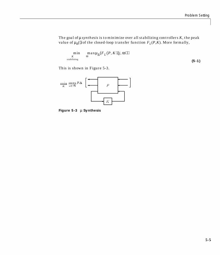
Problem Setting
The goal of µ synthesis is to minimize over all stabilizing controllers K, the peakvalue of µ∆(⋅) of the closed-loop transfer function FL(P,K). More formally,
(5-1)
This is shown in Figure 5-3.
Figure 5-3 µ Synthesis
ωmin maxµ∆ FL P K,( ) j ω,( )( )
Kstabilizing
max
!2RminK
- K
P
5-5
5 Control Design via µ Synthesis
5-6
Replacing µ With its Upper BoundFor tractability of the µ synthesis problem it is necessary to replace µ∆(⋅) withthe upper bound. In Chapter 4, we saw that for a constant matrix M and anuncertainty structure ∆, an upper bound for µ∆(M) is an optimally scaledmaximum singular value,
Recall that Dx∆ is the set of matrices with the property that D∆ = ∆D for everyD ∈ D∆, ∆ ∈ ∆.
Using this upper bound, the optimization in equation (5-1) is reformulated as
(5-2)
Remember, the D minimization is simply an approximation to µ[FL(P,K)(jω)].Dω is chosen from the set of scalings, D∆, independently at every ω. Hence, wehave
(5-3)
By D.,Dω ∈ D∆, we mean a frequency-dependent function D that satisfiesDω ∈ D∆ for each ω. The general expression is notated as ||ƒ||
∞,
giving
(5-4)
Consider a single matrix D ∈ D∆, and a complex matrix M. Suppose that U is acomplex matrix with the same structure as D, but satisfying U*U = UU* = I.Each block of U is a unitary (orthogonal) matrix. Recall that matrix
µ∆ M( ) inf σ DMD 1–( )≤D D∆∈
min max min σ DωFL
P K,( ) jω( )Dω1–[ ]
ωKstabilizing
Dω D∆∈
min min max σ DωFL
P K,( ) jω( )Dω1–[ ]
ωKstabilizing
D.,Dω D∆∈
maxσ f ω( )[ ]ω
min min DFL P K,( )D 1–∞
Kstabilizing
D.,Dω D∆∈

Replacing µ With its Upper Bound
multiplication by an orthogonal matrix does not affect the maximum singularvalue, hence
So, replacing D by UD does not affect the upper bound. Using this freedom inthe phase of each block of D, we can restrict the frequency-dependent scalingmatrix Dω of equation (5-4) to be a real-rational, stable, minimum-phasetransfer function, , and not affect the value of the minimum.
Hence the new optimization is
(5-5)
This optimization is currently solved by an iterative approach, referred to asD – K iteration. A block diagram depicting the optimization is shown in Figure5-4.
Figure 5-4 Replacing µ with Upper Bound
A specific example clarifies some of the ideas. Assume for simplicity that theuncertainty block ∆pert only has full, unmodeled dynamics (ie., complex) blocks,say, N of them. Then the set ∆pert is of the form
(5-6)
σ UD( )M UD( ) 1–[ ] σ UDMD1–
U*[ ]=
σ DMD 1–( )=
Dˆ
s( )
min min Dˆ
FL P K,( )Dˆ 1–
∞K
stabilizingDˆ
s( ) D∆∈stable, min-phase
P
K
D
minK;D
1
-
D1
∆pert diag ∆1 ∆2 … ∆N, , ,[ ] : ∆i Cri ci×
∈
=
5-7

5 Control Design via µ Synthesis
5-8
The set ∆ has the additional fictitious block (for the robust performancecharacterization)
(5-7)
Therefore, the scaling set D∆ is easily seen to be
(5-8)
The elements of D∆, which are defined in (5-8) to be real and positive, can beallowed to take on any nonzero complex values and not change the value of theupper bound, . Using this freedom in the phase of eachentry of D, we can restrict the frequency-dependent scaling matrix Dω ofequation (5-4) to be a real-rational, stable, minimum-phase transfer function,
. The optimization is now
∆ diag ∆1 ∆2 … ∆N ∆F, , , ,[ ] : ∆i Cri ci×
∈ ∆F Cnd ne×
∈,
=
D∆ diag d1I d2I … dNI I, , , ,[ ] : di 0> =
infD D∈ ∆σ DMD 1–( )
d s( )
min
dˆ 1I … 0 0
0 … dˆ NI 00 … 0 I
FL P K,( )
dˆ 1I … 0 0
0 … dˆ NI 00 … 0 I
1–
∞
K d, … …… … … …......
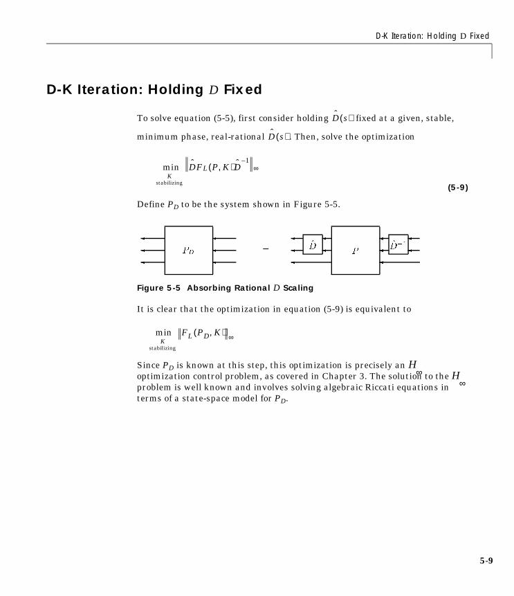
D-K Iteration: Holding D Fixed
D-K Iteration: Holding D Fixed
To solve equation (5-5), first consider holding fixed at a given, stable,
minimum phase, real-rational . Then, solve the optimization
(5-9)
Define PD to be the system shown in Figure 5-5.
Figure 5-5 Absorbing Rational D Scaling
It is clear that the optimization in equation (5-9) is equivalent to
Since PD is known at this step, this optimization is precisely an H∞optimization control problem, as covered in Chapter 3. The solution to the H
∞problem is well known and involves solving algebraic Riccati equations interms of a state-space model for PD.
D s( )
D s( )
min DFL P K,( )D1–
∞K
stabilizing
PD
= P
D
D1
min FL PD K,( ) ∞Kstabilizing
5-9
5 Control Design via µ Synthesis
5-1
D-K Iteration: Holding K Fixed With K held fixed, the optimization over D is carried out in a two-stepprocedure:
1 Finding the optimal frequency-dependent scaling matrix D at a large, butfinite set of frequencies (this is the upper bound calculation for µ).
2 Fitting this optimal frequency-dependent scaling with a stable,minimum-phase, real-rational transfer function .
The two-step procedure is a viable and reliable approach. The primary reasonfor its success is the efficiency with which both of the individual steps arecarried out. The µ upper bound is based on a convex optimization problem. Forthis problem, we have developed many heuristics, which when combined withstandard convex minimization tools leads to a fast, and accurate computationof the upper bound.The fitting algorithm, using genphase and fitsys, is basedon FFT, least squares and again heuristics. It is extremely fast and works wellin most situations.
Two-Step Procedure for Scalar entries d of D We explain the two-step procedure for the case of scalar entries d of the Dscaling matrix, as described earlier. The two-step procedure for full-block Dscalings is covered in the next section.
A stabilizing controller, K(s), is given, and the closed-loop FL(P,K) is formed. Ateach frequency, we solve the minimization corresponding to the upper boundfor µ.
This minimization is done over the real, positive Dω from the set D∆ defined inequation (5-8). This is carried out with µ, in the upper bound optimization.Recall that the addition of phase to each di (ω) does not affect the value of
. In other words, the important aspect of the scaling di
is its magnitude, |di (jω)|.
D
min σ DωFL
P K,( ) jω( )Dω1–[ ]
Dω D∈
σ DωFl
P K,( ) jω( )Dω1–[ ]
0
D-K Iteration: Holding K Fixed
Hence, each positive function, di, which is defined on a finite set of frequencies,is fit (in magnitude) by a proper, stable, minimum-phase transfer function,
. This is accomplished as follows: Use the Bode integral formulae todetermine the phase θi(ω) of the stable, minimum-phase function Li thatsatisfies
|Li(jω)| = di(ω)
for all ω. Then, use the transfer function fitting routine fitsys to construct areal-rational transfer function such that
These rational functions are collected together in a diagonal transfer functionmatrix ,
and absorbed into the original open-loop generalized plant P (to yield PD, asdescribed earlier).
Two-Step Procedure for Full D (Optional Reading) If there are repeated scalar uncertainty blocks, the corresponding blocks of theD matrices are square, full, positive definite Hermitian matrices. Furthermore,at frequencies where M(jω) is a real matrix, the optimal scaling matrix D is alsoreal. Fitting these requires more care than fitting the scalar d scalingsdescribed earlier. We describe the approach used in µ-Tools. Suppose that D :jR → Cn×n is a continuous function, with
1
2 D(0) ∈ Rn×n
3
4
Then, under some smoothness assumptions, we do the following. For each1 ð i ð n,
di s( )
di s( )
di jω( ) ejθi ω( )
di ω( ) Li jω( )=≈phase magnitude
Dˆ
s( )
Dˆ
s( ) diag d1 s( )I d2 s( )I,…dˆ
F 1– s( )I,I,[ ]=
limω ∞→ D jω( )=:D Rn n×∈
ω∀ R D jω( ),∈ D* jω( ) 0>=
D DT 0>=
5-11

5 Control Design via µ Synthesis
5-1
1 Find a stable minimum phase rational function such that for all ω ∈ R,
2 Define a real-valued function φi : R → R such that
3 For each k = 1,2,. . .,i – 1,i + 1,. . .,n, find rational (not necessarily stableor minimum phase) such that for all ω ∈ R,
Now, put all of these rational functions into a matrix
and define Φ := diag[φi]. If the rational fitting was done accurately, then, forall ω
Also, has no poles on the imaginary axis, and has nonzero determinanteverywhere on the imaginary axis. Hence, by spectral factorization techniques(and the command extsmp), we can find a stable, minimum-phase and aunitary matrix function such that
for all ω. The stable, minimum-phase rational matrix is an appropriatescaling for the iteration.
gi
gi jω( ) Dii jω( )≈
ejθi ω( )
:=gi jω( )
gi jω( )-------------------
gik
gik jw( ) ej∅i w( )Dik jw( )≈
Gˆ
s( ) :=
g1 g12 … g1n
g21 g2 … g2n
gn1ˆ gn2
ˆ … gnˆ
……… ...
Gˆ
jω( ) ejΦ ω( )D jω( )=
Gˆ
Dˆ
Uˆ
Gˆ
jω( ) Uˆ
jω( )Dˆ
jω( )=
Dˆ
2

Commands for D – K Iteration
Commands for D – K Iteration Within µ-Tools there are four ways to perform D – K iteration. They are:
1 Use the graphical user interface dkitgui for automated, adjustable, andvisual iterations, which allow for easy monitoring of progress;
2 Use the script file dkit (improved syntax, algorithms and ease-of-use fromversion 2.0) for automated but adjustable iterations;
3 Use the dkit command in the auto mode to run a specified number ofiterations in an automatic mode (requires no user intervention);
4 Write your own iteration loop, using commands such as hinfsyn, frsp, mu,and msf. This approach is not recommended.
5-13
5 Control Design via µ Synthesis
5-1
DiscussionThere are two shortcomings with the D – K iteration control design procedure.
• We have approximated µ∆(⋅) by its upper bound. This is not a serious problemsince the value of µ and its upper bound are often close.
• The D – K iteration is not guaranteed to converge to a global, or even localminimum [SteD]. This is a very serious problem, and represents the biggestlimitation of the design procedure.
In spite of these drawbacks, the D – K iteration control design techniqueappears to work well on many engineering problems. It has been applied withsuccess to vibration suppression for flexible structures, flight control, chemicalprocess control problems, and acoustic reverberation suppression inenclosures.
At this point, we recommend that you proceed to Chapter 7 for examples of theiteration.
References[SteD:] Stein, G., and J. Doyle, “Beyond singular values and loopshapes,”AIAA Journal of Guidance and Control, vol. 14, num. 1, pp. 5-16, January,1991.
4

Auto-Fit for Scalings (Optional Reading)
Auto-Fit for Scalings (Optional Reading) In dkit and dkitgui, there are routines that automatically choose the order ofthe fit. This is done by comparing the effectiveness of the rational fit. Forsimplicity of explanation, consider the situation where all of the uncertaintyblocks are full, so that the D-scaling matrix is made up of several scalarfunctions, di.
Suppose that the kth scaling dk(ω)is fit with an rth order, stable, minimum
phase function . The suitability of this rational fit is
assessed by first defining a scaling matrix
Note that in this matrix we have simply replaced the optimalfrequency-by-frequency scaling dk (obtained in the µ upper bound computation)with the frequency response of the rational fit . Next, we compare the valuesof
If these are close, then r is deemed a suitable order for the kth scaling functiondk. The measure of closeness can be chosen. Define
dk s( ) ejθk ω( )
dk ω( )≈
Dk r, ω( ) :=
d1 ω( ) … 0 0 0 … 0
0 0 0 … 00 … dk 1– ω( ) 0 0 … 0
0 … 0 dk jω( ) 0 … 0
0 … 0 0 dk 1+ ω( ) … 0
…0 … 0 0 0 … I
...
...
…… … … ……
dk
σ D ω( )FL(P K) jω( )D 1– ω( ),[ ] and σ D k r,[ ] ω( )FL(P K) jω( )D k r,[ ]1– ω( ),[ ]
β := maxσ D ω( )FL(P K) jω( )D 1– ω( ),[ ]ω R∈
5-15

5 Control Design via µ Synthesis
5-1
Our rules are as follows: For frequencies where
we require that
The quantity 1.03 is the AutoTol parameter in dkit which can be modifiedeasily. In dkitgui, the Auto-Fit Tolerance which is adjustable in theParameter window varies this parameter from 1.01 (tight) to 1.06 (loose).
For other frequencies, we require that
Note that the order of is chosen based on its performance as a scaling whileall of the other scalings are set to their optimal (dk(ω)). You can easily modifythe constants 0.5 and 0.1 to demand tighter tolerance on the autofittingalgorithm.
σ D ω( )FL(P K) jω( )D 1– ω( ),[ ] 0.5β≥
σ Dk r, ω( )FL(P K) jω( )Dk r,1– ω( ),[ ] 1.03σ D ω( )FL(P K) jω( )D 1– ω( ),[ ]≤
σ Dk r, ω( )FL(P K) jω( )Dk r,1– ω( ),[ ] σ D ω( )FL(P K) jω( )D 1– ω( ),[ ] 0.1β+≤
dk
6

6
Graphical User InterfaceTools
6 Graphical User Interface Tools
6-2
This chapter describes three µ-Analysis and Synthesis Toolbox (µ-Tools)graphical user interface tools:
• Workspace tool: wsgui
• D – K Iteration tool: dkitgui
• Simulation tool: simgui
The functionality and application of these tools is illustrated with amultivariable control problem.

Workspace User Interface Tool: wsgui
Workspace User Interface Tool: wsgui The µ-Tools Workspace Manager, wsgui, is used to view variables in theworkspace, drag them to other µ-Tools graphical user interface (GUI) dropboxes, and export variables from the µ-Tools user interfaces to the workspace.In this section we only describe how the tool is used to view the workspacevariables. In other sections we will show how the tool integrates with otherµ-Tools GUI tools.
Clear the workspace, create the weighting functions used in the Shuttleexample, and start the Workspace Manager.
clear; mk_wts; wsgui
The wsgui Workspace Manager window appears as in Figure 6-1.
Each time Refresh Variables is pressed, the MATLAB command who isexecuted, and minfo is run to determine the variable type and dimension. Thisinformation is displayed in the main scrollable table. The date and time of thelast Refresh are displayed below the button.
6-3

6 Graphical User Interface Tools
6-4
Figure 6-1 Initial wsgui Main Window
The scrollable table can be moved up/down one page by pressing above/belowthe slider. Pressing the arrows at the end of the slider moves the table one line.
A filter is used to make viewing of a reduced number of selections easy. ThePrefix, Suffix, and matrix type filters are on the bottom of the scrollabletable. The matrix type filter is a pop-up menu to the right of Suffix. Forinstance, let’s look at SYSTEM matrices whose names begin with w. Type a win the Prefix box, as shown in Figure 6-2. Note that the Apply Selectionbutton becomes enabled, yet all 20 matrices in the workspace are still displayed(even those that don’t start with a w). The selection filter is only applied whenyou press the Apply Selection button. Move to the right to the pop-up menu,which currently displays All, and select System, as shown in Figure 6-2. TheApply Selection remains enabled, and again, matrices that are not SYSTEMmatrices are still displayed. Press Apply Selection to apply the filter (first

Workspace User Interface Tool: wsgui
letter = w, matrix type = SYSTEM). The scrollable table refreshes, leaving 7 (ofthe original 20) matrices displayed, as seen in Figure 6-3.
Figure 6-2 wsgui Main Window with Selected Options
6-5

6 Graphical User Interface Tools
6-6
Figure 6-3 wsgui Main Window After Apply Selection
Now, go into the MATLAB command window, and create a new SYSTEMmatrix, with first letter w
wnew = nd2sys([1 2],[1 2 3 4]);
Note that this does not immediately appear in the scrollable table, even thoughit satisfies the selection criteria. This new variable will not appear until theRefresh Variables button is pushed. Press the Refresh Variables button andnote that when the table is refilled, the system wnew appears as expected,Figure 6-4.

Workspace User Interface Tool: wsgui
Figure 6-4 wsgui Main Window
Often, you want to create a more complicated selection criteria. The Customfilter can be used to do this. Press the push button marked with a * (to the rightof the matrix type pop-up menu) to switch to the Custom filter. Lets find allmatrices with four or more outputs. In the Custom box, type
ynum(mdata)>=4
and press Apply Selection. The results are shown in Figure 6-5. This willevaluate the expression in the Custom box, and select those workspacevariables for which the expression is true. In the Custom box, use mdata toindicate the matrix’s value, and mname to substitute the matrix’s name. Hence,selections can be based on the name and value of any workspace variable.
6-7

6 Graphical User Interface Tools
6-8
Figure 6-5 wsgui Main Window with Custom Selection Open
File MenuThe File menu at the top of the Workspace Manager window has three menuitems as seen in Figure 6-6.
Figure 6-6 File Menu
The Clear Selected Matrices item allows you to clear the variable namescurrently appearing in the Workspace Manager window from the MATLAB
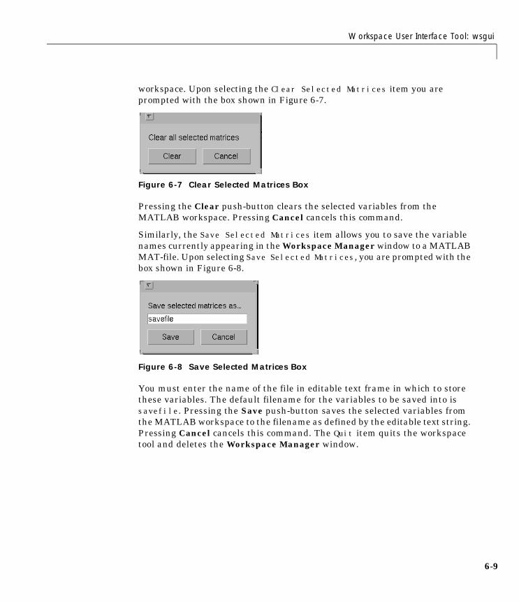
Workspace User Interface Tool: wsgui
workspace. Upon selecting the Clear Selected Matrices item you areprompted with the box shown in Figure 6-7.
Figure 6-7 Clear Selected Matrices Box
Pressing the Clear push-button clears the selected variables from theMATLAB workspace. Pressing Cancel cancels this command.
Similarly, the Save Selected Matrices item allows you to save the variablenames currently appearing in the Workspace Manager window to a MATLABMAT-file. Upon selecting Save Selected Matrices, you are prompted with thebox shown in Figure 6-8.
Figure 6-8 Save Selected Matrices Box
You must enter the name of the file in editable text frame in which to storethese variables. The default filename for the variables to be saved into issavefile. Pressing the Save push-button saves the selected variables fromthe MATLAB workspace to the filename as defined by the editable text string.Pressing Cancel cancels this command. The Quit item quits the workspacetool and deletes the Workspace Manager window.
6-9

6 Graphical User Interface Tools
6-1
Options MenuThe Options menu at the top of the Workspace Manager window has threemenu items, as seen in Figure 6-9.
Figure 6-9 Options Menu
The CleanUp item redisplays the variable names and data appearing in theWorkspace Manager window. The other two menu items are Font and # of Lines. These items correspond to the font type and number of items shown inthe workspace window. The Font menu item allows you to select a font size of7 to 12 to display the data (see Figure 6-10). The # of Lines menu item allowsyou to select the number of lines of data displayed in the workspace window.You can select between [12 20 28 36 44] lines of data. This is especially usefulsince the Workspace Manager window is resizable.
Figure 6-10 Font and # of Lines Menu Items
Note: You must select the CleanUp item from the Options menu afterresizing.
0

Workspace User Interface Tool: wsgui
Export ButtonThe Export button and editable text boxes at the bottom of the WorkspaceManager window allow you to export data from other µ-Tools user interfacesto the MATLAB workspace. The Export button also allows you to copyworkspace variables, although it is just as easy to do this at the MATLABcommand line.
Consider the following example of how to copy variables. Select all theSYSTEM matrices currently in your MATLAB workspace. To copy the wpSYSTEM matrix to the variable TEMP, type wp in the editable text box to theright of the Export button and TEMP in the editable text box to the right of As.Your Workspace Manager window should correspond to Figure 6-11.
Pressing the Export button copies wp to the variable TEMP in your MATLABworkspace. The text display in the message bar shows the MATLAB commandand the time and date it was executed. Your Workspace Manager windowshould look like Figure 6-12 after the Refresh Variables button is pressed. Thedrop box to the right of the Export button provides another manner to depositinformation to be copied into the workspace. For more information about howto use µ-Tools drop boxes see the “Dragging and Dropping Icons” section of thischapter.
6-11
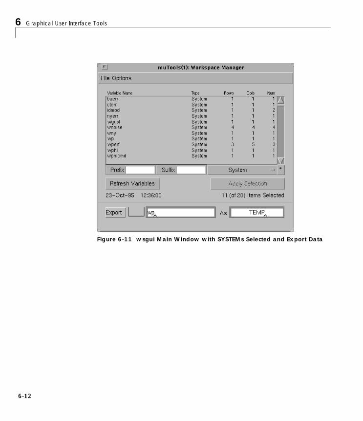
6 Graphical User Interface Tools
6-1
Figure 6-11 wsgui Main Window with SYSTEMs Selected and Export Data
2

Workspace User Interface Tool: wsgui
Figure 6-12 wsgui Main Window After Refreshing Exported Data
6-13

6 Graphical User Interface Tools
6-1
Spinning Satellite Example: Problem StatementIn this section we describe an example application that will be used in thefollowing two sections to demonstrate µ-analysis and synthesis methods usingµ-Tools graphical user interfaces.
Consider a satellite spinning about its z-axis with a control objective tominimize the x and y-axes rotations due to x and y-axes disturbances. Thecontrol inputs are torque actuators in the x and y-axis and the feedbackmeasurements are angular sensors. In this example the sensor measurementsare poorly aligned with the axis of rotation being measured. The pooralignment of the sensor measurements is introduced on purpose to illustratethe importance of direction in a multivariable control problem.
The following are the linear, state equations of the satellite:
Therefore, the nominal state-space model for the spinning satellite is defined as
ddt------
Θx
Θy
0 1010– 0
Θx
Θy
0 11 0
u1
u2
+=
y1
y2
1 1010– 1
Θx
Θy
=
GAG BG
CG DG
0 10 1 010– 0 0 11 10 0 010– 1 0 0
= =
4

Spinning Satellite Example: Problem Statement
The spinning satellite has the following characteristics that need to be includedin the control problem formulation:
• The model of the channel 1 actuator has uncertainty or error of 20% at lowfrequency, below 1 rad/sec. This modeling error reaches 100% uncertainty at20 rad/sec with very large potential errors in this actuator model above 200rad/sec. We choose to model this in the µ framework as a multiplicative inputuncertainty. A frequency domain weight is constructed to describe thepercentage modeling error as a function of frequency. The multiplicativeuncertainty weight associated with the first actuator is
A frequency response plot of this weight is shown in Figure 6-13.
Figure 6-13 Uncertainty Weights: Wdel1 (solid), Wdel2 (dashed)
Wdel1 := 10 s 4+( )s 200+
------------------------
102
101
100
101
102
103
104
101
100
101
Frequency (rad/sec)
Mag
nitu
de
W_del1 (solid) and W_del2 (dashed)
6-15
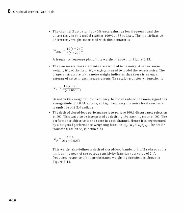
6 Graphical User Interface Tools
6-1
• The channel 2 actuator has 40% uncertainty at low frequency and theuncertainty in this model reaches 100% at 58 rad/sec. The multiplicativeuncertainty weight associated with this actuator is
A frequency response plot of this weight is shown in Figure 6-13.
• The two sensor measurements are assumed to be noisy. A sensor noiseweight, Wn, of the form Wn = wnI2×2 is used to model the sensor noise. Thediagonal structure of the noise weight indicates that there is an equalamount of noise in each measurement. The scalar transfer wn function is
Based on this weight at low frequency, below 20 rad/sec, the noise signal hasa magnitude of ± 0.01radians, at high frequency the noise level reaches amagnitude of ± 2.4 radians.
• The desired closed-loop performance is to achieve 100:1 disturbance rejectionat DC. This can also be interpreted as desiring 1% tracking error at DC. Theperformance objective is the same in each channel. Hence it is representedby a diagonal performance weighting function Wp, Wp = wpI2×2. The scalartransfer function wp is defined as
This weight also defines a desired closed-loop bandwidth of 2 rad/sec and alimit on the peak of the output sensitivity function to a value of 2. Afrequency response of the performance weighting functions is shown inFigure 6-14.
Wdel2 := 10 s 24+( )3 s 200+( )---------------------------
wn := 12 s 25+( )5 s 6000+( )------------------------------
wp =s 4+
2 s 0.02+( )-----------------------------
6

Spinning Satellite Example: Problem Statement
Figure 6-14 Performance Weights: Wp (solid), Wn (dashed)
The control design block diagram for the spinning satellite is shown in Figure6-15. The uncertainty weights, Wdel1 and Wdel2, and the performance weights,Wp and Wn, are design parameters that you, the control engineer, canmanipulate. These weights are used to incorporate information about thephysical system into the control design.
102
101
100
101
102
103
104
102
101
100
101
102
Frequency (rad/sec)
Mag
nitu
de
W_p (solid) and W_n (dashed)
6-17
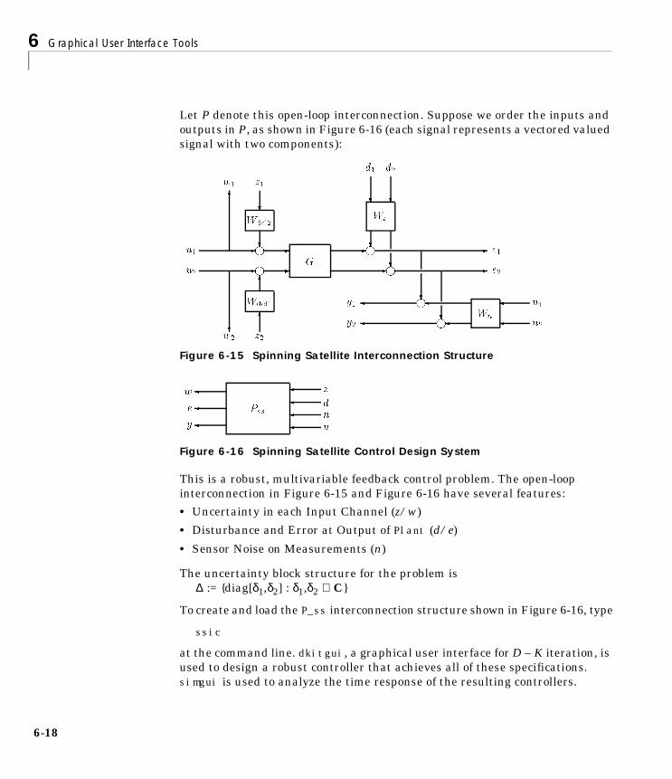
6 Graphical User Interface Tools
6-1
Let P denote this open-loop interconnection. Suppose we order the inputs andoutputs in P, as shown in Figure 6-16 (each signal represents a vectored valuedsignal with two components):
Figure 6-15 Spinning Satellite Interconnection Structure
Figure 6-16 Spinning Satellite Control Design System
This is a robust, multivariable feedback control problem. The open-loopinterconnection in Figure 6-15 and Figure 6-16 have several features:
• Uncertainty in each Input Channel (z/w)
• Disturbance and Error at Output of Plant (d/e)
• Sensor Noise on Measurements (n)
The uncertainty block structure for the problem is∆ := diag[δ1,δ2] : δ1,δ2 ∈ C
To create and load the P_ss interconnection structure shown in Figure 6-16, type
ssic
at the command line. dkitgui, a graphical user interface for D – K iteration, isused to design a robust controller that achieves all of these specifications.simgui is used to analyze the time response of the resulting controllers.
u1
u2
e1
e2
n1
n2
y1
y2
d1 d2
w1 z1
w2 z2
G
Wdel1
Wdel2Wp
Wn
-
-
-
-
-
-
-
-
6
?6
6g
?
?g
? ?
?g
?g
?g
?g
z
dn
u
w
e
y
Pss
8

D-K Iteration User Interface Tool: dkitgui
D-K Iteration User Interface Tool: dkitguiIn this section we describe the graphical user interface for µ-synthesis viaD – K iteration, an approach to robust control design. The GUI-tool for D – Kiteration is created by the command dkitgui. There are five windowsassociated with this tool. They are the:
• Main Iteration window, which is the main interface for the user during theiteration.
• Setup window, where initial data is entered.
• Parameter window, which is occasionally used to modify properties of the D– K iteration, such as H∞ parameters, and to select the variables that areautomatically exported to the workspace each iteration.
• Frequency Response window, where the plots of µ and of the closed-looptransfer function matrix are displayed.
• Scaling window, where the rational fits of the frequency-dependent D-scaledata are shown, and can be modified.
The spinning satellite control design example from the previous section is usedto illustrate the basic features of dkitgui. Start the tool by typing
dkitgui
Depending on the computer, dkitgui takes up to a minute to start. The main interactive window finally displays the message
Ready for data, Press SETUP to begin
in its lower left corner, as shown in Figure 6-17. This is the location of themessage bar where information about the D – K iteration is displayed.
σ
6-19

6 Graphical User Interface Tools
6-2
Figure 6-17 Initial dkitgui Main Window
Press the SETUP button as instructed. This brings the Setup window to theforeground. The Setup window is shown in Figure 6-18.
0

D-K Iteration User Interface Tool: dkitgui
Figure 6-18 Initial dkitgui Setup Window
To start an iteration, you must enter the following items:
• Open-loop interconnection structure
• Number of uncertainty blocks
• Sizes of the uncertainty blocks
• Sizes of the performance transfer functions (errors and disturbances)
6-21

6 Graphical User Interface Tools
6-2
• Sizes of the feedback signals (measurements and controls)
• Frequency response range
You can enter this information in any order, except that the dimensions of theuncertainty blocks can only be specified after entering the number ofuncertainty blocks. All data entry points are uicontrol editable text objects,and operate in a machine dependent manner with which you should befamiliar. As before, when we instruct you to enter data in an editable textobject, this implicitly means enter the text, and complete the action (bypressing Return, by pressing the mouse on another object, by moving themouse pointer out of the text object, etc.). See the MATLAB Function Referenceonline for more details on completing a text entry.
Notice that three items in the Setup window — Controller, Iteration Suffix, and Iteration Name — are enclosed in < >. This notation denotes avariable that is optional, and no action is necessary.
Enter P_ss (the open-loop interconnection) in the open-loop editable text frame(see Figure 6-19). Press the Open-Loop IC checkbox to load the data into theOpen-Loop IC variable. The pointer turns into an hourglass while MATLABloads the data. Upon loading the data, the pointer turns back into an arrow,and the matrix type (S for System, C for Constant, and V for Varying) of theOpen-Loop IC variable and its dimensions are displayed to the right of theeditable text. In this example the variable P_ss is a SYSTEM matrix with sixoutputs, eight inputs, and eight states. The <Controller> data is optional.This allows you to load an initial controller to start the D – K iteration or duringthe D – K iteration you may want to load a reduced order controller.
Figure 6-19 Open-Loop/Controller Input Frame
Since there are two uncertain actuators in the spinning satellite problem, theuncertainty structure has 2, 1-by-1 uncertainty blocks. Enter a 2 in theUncertainty Structure # of Blocks text field. This opens a 2-by- 3 editablematrix, as seen in Figure 6-20, where the dimensions of the uncertainty blocksare entered. Enter a 1 for each row and column dimension. The third column,labeled Fac, is used for scaling the size of the uncertainty during the iteration.
2

D-K Iteration User Interface Tool: dkitgui
The value of Fac may be varied from.1 to 10, effectively reducing or increasingthe size of the uncertainty by a factor of 10. Leave these factors as 1 for the timebeing.
Figure 6-20 Uncertainty Structure Frame
In the spinning satellite problem (Figure 6-16), there are four exogenousdisturbances (two disturbance torques and two measurement noises) and twopenalized errors (two tracking errors). Enter a 2 in the # of Errors editable textand a 4 into the # of Disturbances editable text in the PerformanceStructure frame. The spinning satellite has two measured variables forfeedback and two control actuators. Enter these in the # of Measurements and# of Controls editable text, respectively, in the Feedback Structure frame.
Drop Box DataIn the right column of the Setup window are push-button with the variablesnames Uncertainty, Performance, Feedback, and Omega, as seen in Figure6-21.
Figure 6-21 Uncertainty, Performance, Feedback, and Omega Frame
Entering data with these push-button is optional. These push-button are usedto enter the same data as SIGNAL DIMENSIONS and Frequency Range
6-23

6 Graphical User Interface Tools
6-2
data. To the left of each push-button is a drop box and to the right of eachpush-button is an editable text box. Data that is dropped into the drop boxes orentered in the editable text overwrites the data in the left column of the Setupwindow. (See the “Dragging and Dropping Icons” section at the end of thischapter for more details.) For example, instead of entering a 2 into the # ofBlocks text and 1, 1, 1, and 1 into each block structure, you could typeones(2,2) in the Uncertainty editable text and press the Uncertaintypush-button. This action overloads this data into the Uncertainty Structure byredrawing the Uncertainty Structure frame and filling out the correspondingeditable text locations. Similarly the Performance data overwrites thePerformance Structure data, Feedback overwrites the Feedback Structuredata, and Omega overwrites the Frequency Range data.
Completing Problem SetupTo complete the problem setup, enter the frequency response informationappropriate for the problem in the Frequency Range frame. Keep theLogspace option, and enter 0.001 for the Low frequency, 100 for the Highfrequency, and 60 in the # Points editable text. Selecting the Custom optionallows you to enter any valid MATLAB expression in the editable text frame.
This completes the input of the data required by dkitgui to start a D – Kiteration. Upon correctly entering the required data, the message
Mu-Synthesis Problem Specification Complete...
appears in the message bar of the Setup window.
Enter text in the optional fields Iteration Suffix and Iteration Name.Iteration Suffix is used for data that is automatically exported to theworkspace. This string is appended to default names for the variables as theyare exported to the workspace. Enter ss in the editable text suffix box. We willsee the precise effect of this later in the example. The Iteration Name modifiesthe title of each figure. Enter Spinning Satellite in the editable text frame,and notice its effect. The Setup window should appear as in Figure 6-22.
4

D-K Iteration User Interface Tool: dkitgui
Figure 6-22 dkitgui Setup Window After Entering Data
To continue with the D – K iteration, first hide the Setup window. This is doneby pulling down the Window menu and selecting Hide Setup from the menuand returning to the main window. Now select the Parameters window fromthe Window menu.
6-25

6 Graphical User Interface Tools
6-2
DK Iteration Parameters WindowThe fifth window titled Parameters, shown in Figure 6-23, contains additionaldata you may want to enter for the D – K iteration. This window is shown ifParameters is selected from the Windows menu. All of the parameters in thiswindow are set to default values. No data entry is required and you can returnto the main Iteration window to initiate the first iteration. The Parameterswindow contains five settings you can change. They are:
• HinfSyn Parameters
• Structured Singular Value (Mu)
• Riccati Solver
• D-scale Prefit
• Each Iteration Export
Figure 6-23 D – K Iteration Parameter Window
6

D-K Iteration User Interface Tool: dkitgui
The HinfSyn Parameters and Riccati Solver settings, shown in Table 6-1,correspond to the inputs of the H∞ control design program hinfsyn. GammaMin and Gamma Max are the minimum and maximum γ values.
The Suboptimal Tol is how close to the optimal γ value is desired. TheImaginary Tol and Positive Def Tol are epr and epp in the hinfsyn program.They correspond to the measure of when the real part of an eigenvalue of theHamiltonian matrices is zero and determination of the positive definiteness ofthe X∞ and Y∞ solutions. The current default value for each parameter is shownin parentheses, ( ), to the right of each label. The Riccati Solver has a mutuallyexclusive set of buttons for selecting either the Schur or Eigenvalue method tobe used to solve the H∞ Riccati equations.
The HinfSyn Parameters frame also allows you to deselect the measurementsand controls used during the control design process. For the spinning satelliteexample there are two controls and two measurements. The MeasurementsUtilized frame indicates that all measurements are currently being used. Youcan input to the Measurements Utilized editable text a standard MATLABvector to denote the measurements that are to be used. Similarly, you canselect in the Controls Utilized frame which control inputs are to be used. Theresulting control design will have zeros in the state space B or C matrix of thecontroller corresponding to the measurements inputs or control outputs thathave been deselected.
The Structured Singular Value (Mu) settings frame has two sets of options.These options correspond to calculation of the structured singular value (µ)using the mu program during D – K iteration. The first set of buttons ismutually exclusive. You can either select to use greatest accuracy or a less
Table 6-1 HinfSyn Parameters and Riccati Solver Frames
Hinfsyn Parameters Riccati Solver
• Gamma Min • Schur Method
• Gamma Max • Eigenvalue Method
• Suboptimal Tol
• Imaginary Tol
• Pos Def Tol
6-27

6 Graphical User Interface Tools
6-2
accurate but faster technique for calculating µ. (The Optimal method calls themu program with the option 'c,' Fast method calls mu with the 'f' option). Youcan also select to calculate only an upper bound for µ which calls mu with the 'U'option. Selecting this option speeds up the µ calculation, but you will be unableto see how different the upper and lower µ bounds are when they are calculatedand plotted in the Mu/SVD Plot window.
The D-Scale Prefit frame contains settings for calculation of the rationalD-scales. The Max Auto-Order defines the maximum D-scale state order to beused to fit an individual D-scaling during the prefitting part of the D-scalesfitting routine. The Max Auto-Order default is five states. The Auto-FitTolerance scroll bar allows you to define how close the rational scaled µ upperbound is to approximate the actual µ upper bound in a norm sense. SelectingLoose will result in lower order D-scales being used in the D-scale prefitting,whereas selecting Tight will likely result in higher order D-scales during theD-scale prefit computation. This setting can play an important role indetermining which minimum of the D – K iteration is achieved. Currently thisis done by trial and error.
The Each Iteration: Export... frame shows data in the form of radio buttonsthat is available to be exported to the MATLAB workspace. In the followinglist, a subscript i denotes that the integer iteration number is added to thevariable’s name. These variables are:
• Controller, which is exported as Ki.
• Mu Analysis exports mubndi, ddatai, dsensi, and perti. The mubndi variableis selected based on the Structured Singular Value (Mu) frame. This isnormally the upper and lower bounds for µ. The ddatai is the D-scale data,dsensi is the sensitivity, and perti is the worst-case perturbation as afunction of frequency. These are the standard outputs of the mu function.
• Closed-Loop Freq Response exports the closed-loop system, clpi, and itsfrequency response clpig.
• Rational D-scalings exports the left, dli, and right, dri, rational D-scalings.
• Open-Loop Interconnection is exported as olici.
The Iteration Suffix string, which was input in the Setup window, is appendedto the end of all the output variables selected in the Each Iteration: Export...frame. In this example, the Controller and the Mu Analysis data is selectedfor output. Therefore after the Control Design button executes for the firsttime, the variable K1ss will be in the workspace.
8
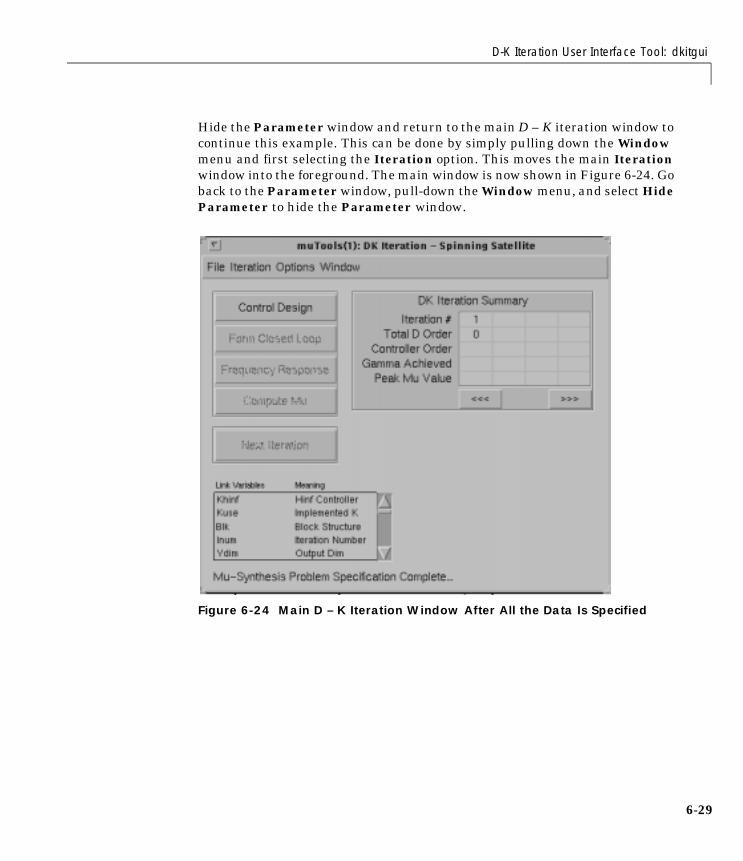
D-K Iteration User Interface Tool: dkitgui
Hide the Parameter window and return to the main D – K iteration window tocontinue this example. This can be done by simply pulling down the Windowmenu and first selecting the Iteration option. This moves the main Iterationwindow into the foreground. The main window is now shown in Figure 6-24. Goback to the Parameter window, pull-down the Window menu, and select HideParameter to hide the Parameter window.
Figure 6-24 Main D – K Iteration Window After All the Data Is Specified
6-29
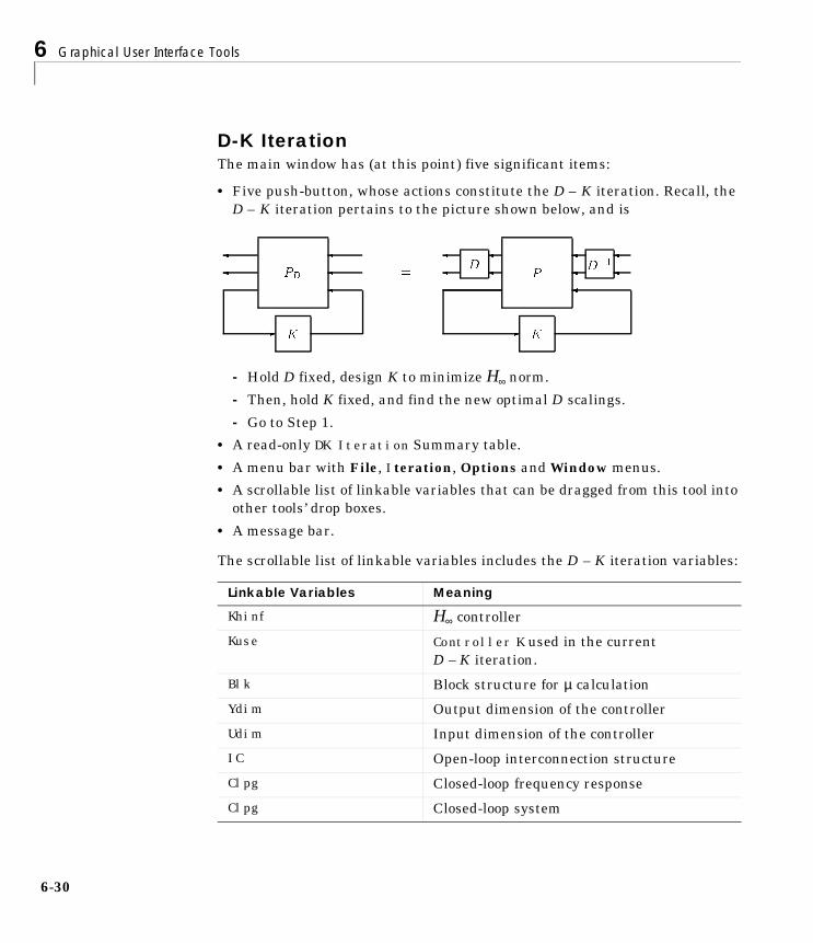
6 Graphical User Interface Tools
6-3
D-K IterationThe main window has (at this point) five significant items:
• Five push-button, whose actions constitute the D – K iteration. Recall, theD – K iteration pertains to the picture shown below, and is
- Hold D fixed, design K to minimize H∞ norm.
- Then, hold K fixed, and find the new optimal D scalings.
- Go to Step 1.
• A read-only DK Iteration Summary table.
• A menu bar with File, Iteration, Options and Window menus.
• A scrollable list of linkable variables that can be dragged from this tool intoother tools’ drop boxes.
• A message bar.
The scrollable list of linkable variables includes the D – K iteration variables:
Linkable Variables Meaning
Khinf H∞ controller
Kuse Controller K used in the currentD – K iteration.
Blk Block structure for µ calculation
Ydim Output dimension of the controller
Udim Input dimension of the controller
IC Open-loop interconnection structure
Clpg Closed-loop frequency response
Clpg Closed-loop system
PD
- K
= P
D
D1
- K
0

D-K Iteration User Interface Tool: dkitgui
These variables can be dragged and dropped at anytime into other µ-Tools userinterface commands.
The Control Design push-button is enabled, and is the first step of theiteration. At this point, the D matrices are set to identity (of appropriatedimension). Design the first H∞ controller by pressing the Control Designbutton. The standard gamma iteration data from hinfsyn is displayed in theMATLAB command window. The DK Iteration Summary table is updated atthe end of the control design, and the Form Closed-Loop button is enabled.
The next two steps are simple — form the closed-loop system, and calculateclosed-loop frequency response. Press the Form Closed-Loop and FrequencyResponse buttons as they are enabled. As the frequency response of theclosed-loop system is calculated, a running tab of the number of frequencypoints calculated is shown in the message frame of the main window. The normof the closed-loop transfer function as a function of frequency is plotted in theFrequency Response window as seen in Figure 6-25. (Note that Figure 6-25includes the µ plot, which is not accurate at this point in the D – K iteration.)In general, this transfer function has the D-scalings from the previous iteration(for the first iteration it’s just identity) and the controller which was justdesigned. Upon completing the frequency response the Compute Mu button isenabled.
Now, compute the structured singular value, µ, of the closed-loop frequencyresponse by pressing the Compute Mu button. The block structure was definedin the Setup window, in the Block Structure field. Recall (see Chapter 4) thatthe upper bound for µ is computed by determining the optimal D-scalings as afunction of frequency. Like the frequency response, a running tab of the µcalculation is shown in the message frame of the main window. The results areshown in Figure 6-25.
6-31

6 Graphical User Interface Tools
6-3
Figure 6-25 µ Upper Bound and Maximum Singular Value for First D – K Iteration
You have now completed one D – K iteration. The DK Iteration Summary tableis completely updated for the first iteration, as shown in Figure 6-26. The NextIteration button is highlighted. Once the Next Iteration button is pushed youcannot effectively return to the previous iteration.
Suppose you desire a more refined frequency response for the µ calculation.You can do this before you move to the second iteration by changing the datain the Frequency Range frame in the Setup window. Changing the number offrequency response points from 60 to 80 results in the <Frequency Response>button being enabled. Note that the sideways carrots < > around the buttonname denote that you may select the frequency response or go to the nextiteration. Continuing to the next iteration without pressing the Frequencybutton will not change any of the data calculated during the first iteration.
2
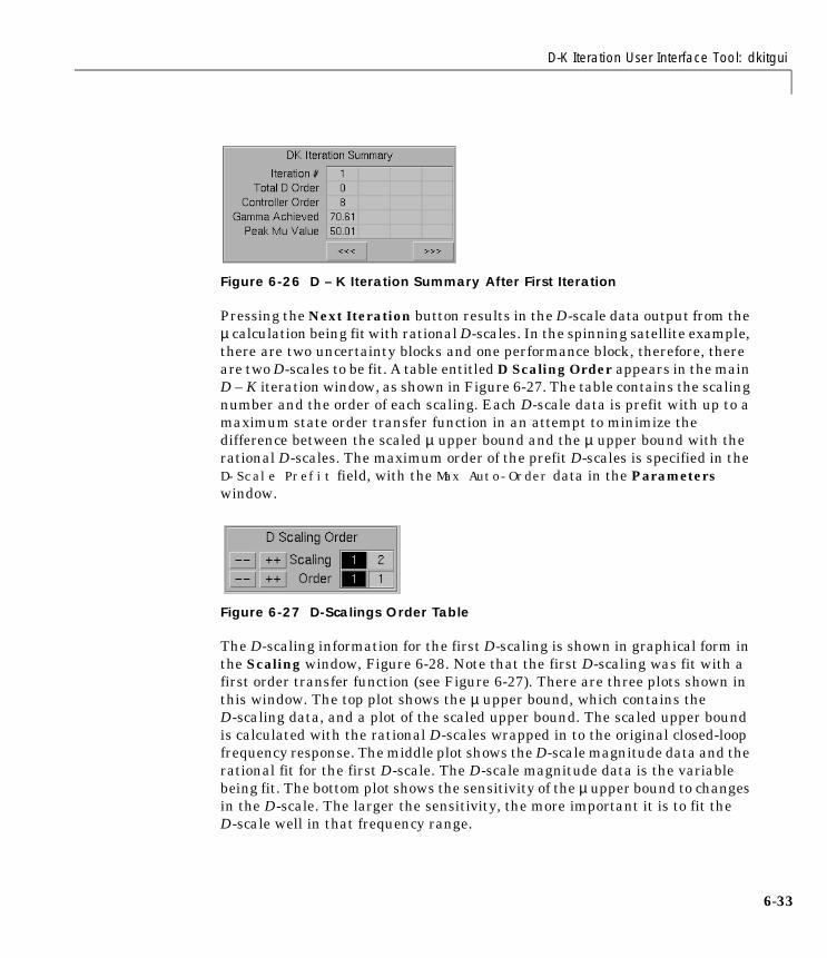
D-K Iteration User Interface Tool: dkitgui
Figure 6-26 D – K Iteration Summary After First Iteration
Pressing the Next Iteration button results in the D-scale data output from theµ calculation being fit with rational D-scales. In the spinning satellite example,there are two uncertainty blocks and one performance block, therefore, thereare two D-scales to be fit. A table entitled D Scaling Order appears in the mainD – K iteration window, as shown in Figure 6-27. The table contains the scalingnumber and the order of each scaling. Each D-scale data is prefit with up to amaximum state order transfer function in an attempt to minimize thedifference between the scaled µ upper bound and the µ upper bound with therational D-scales. The maximum order of the prefit D-scales is specified in theD-Scale Prefit field, with the Max Auto-Order data in the Parameterswindow.
Figure 6-27 D-Scalings Order Table
The D-scaling information for the first D-scaling is shown in graphical form inthe Scaling window, Figure 6-28. Note that the first D-scaling was fit with afirst order transfer function (see Figure 6-27). There are three plots shown inthis window. The top plot shows the µ upper bound, which contains theD-scaling data, and a plot of the scaled upper bound. The scaled upper boundis calculated with the rational D-scales wrapped in to the original closed-loopfrequency response. The middle plot shows the D-scale magnitude data and therational fit for the first D-scale. The D-scale magnitude data is the variablebeing fit. The bottom plot shows the sensitivity of the µ upper bound to changesin the D-scale. The larger the sensitivity, the more important it is to fit theD-scale well in that frequency range.
6-33
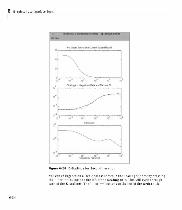
6 Graphical User Interface Tools
6-3
Figure 6-28 D-Scalings for Second Iteration
You can change which D-scale data is shown in the Scaling window by pressingthe '- -' or '++' buttons to the left of the Scaling title. This will cycle througheach of the D-scalings. The '- -' or '++' buttons to the left of the Order title
4

D-K Iteration User Interface Tool: dkitgui
decrement or increment the order of the D-scale fit by 1. You can also changethe order of the D-scale fit by editing the D-scale order directly. Changing theD fit order will affect the middle plot, which shows the magnitude data (solidline) and the rational fit (dashed line) and will also affect the current scaledupper bound (dashed line) shown in the top figure of the Scaling window. Notethat the goal of D – K iteration is to reduce the µ upper bound. It is usuallyimportant that the current scaled upper bound, which incorporates the rationalD-scalings, closely matches the calculated µ upper bound. This is especiallytrue in the frequency range where µ is large.
The D-scale data for this example are both fit with first order transferfunctions. These fits appear to be sufficient, therefore we will go on to thesecond control design. Pressing the Control Design button wraps the rationalD-scalings into the original interconnection structure, P_ss, and designs a newH∞ controller. For this second D – K iteration, a γ value of 7.89 is achieved.
We now desire to run the next three buttons in sequence. This can be done bypulling down the Iteration menubar in the main Iteration window. SelectingAuto Steps, dragging the mouse to the right of Auto Steps allows you to choosethe menu item Next 3 Steps, as shown in Figure 6-29. This automatically runsthe next three steps of the D – K iteration. Selecting either the Auto Steps orAuto Iterate will result in the appearance of a Stop button in the mainIteration window below the DK Iteration Summary table. Pressing the Stopbutton terminates the automated D – K iteration after the current buttonrunning has completed.
Figure 6-29 Main Window Iteration Pull-down Menu
Under the Iteration menu, the Restart option allows you to restart a D – Kiteration at the very beginning while leaving the Setup window data intact.This is often useful if the incorrect weights were selected and you would like toreload the system interconnection structure and start over.
6-35

6 Graphical User Interface Tools
6-3
Note that after two complete D – K iterations we have achieved a µ value of 2.11(Figure 6-30). The objective is to achieve a µ value less than 1. Therefore,several more D – K iterations may be required. User interaction can beeliminated from the D – K iteration by selecting the Auto Iterate menu itemfrom the DK Iteration window, Iteration menubar, as shown in Figure 6-31.Dragging the mouse to the right of the Auto Iterate menu item allows you toselect up from one to eight automated D – K iterations. During each iteration,the rational D-scale order is selected automatically by the dkitgui program.Again, the Stop button allows you to terminate the Auto Iterate option at anytime. After three complete D – K iterations, a µ value of 1.03 is achieved.Selecting one more automated D – K iteration results in a µ value of 0.91 afterfour iterations (Figure 6-32).
Figure 6-30 D – K Iteration Summary After Two Iterations.
Figure 6-31 Main Window Iteration Pull-down Menu
6

D-K Iteration User Interface Tool: dkitgui
Figure 6-32 D – K Iteration Summary After Four Iterations
Based on the setting of the Each Iteration Export radio buttons in theParameter window, the controller designed each iteration has been exportedto the MATLAB workspace. Therefore, after four D – K iterations controllersK1ss, K2ss, K3ss, and K4ss are present in your workspace. We also have datafrom the µ analysis, ddataiss, desnsiss, mubndiss, and pertiss in theworkspace. If you have your Workspace Manager open, press the RefreshVariables button. The results are shown in Figure 6-33.
6-37

6 Graphical User Interface Tools
6-3
Figure 6-33 Data in the MATLAB Workspace After Four D – K Iterations
We have successfully designed a controller to achieve our objectives since µ isless than 1. To quit the D – K iteration graphical user interface, pull down theFile menu from the main Iteration window and highlight the Quit option.
Options MenuThe Options menu in the main dkitgui window allows you to perform twospecialized operations. Selecting the Auto_Refresh K item from the Optionsmenu will refresh the <Controller> editable text in the Setup window after
8

D-K Iteration User Interface Tool: dkitgui
successful completion of the Control Design button. Any valid MATLABexpression can be typed in the <Controller> editable text space. This allowsyou to perhaps have an automated controller reduction scheme that would getexecuted after the design of the H∞ controller.
Figure 6-34 D – K Options Menu
Selecting the Auto_Refresh Olic item from the Options menu will refresh theOpen-Loop IC editable text in the Setup window after successful completionof the fitting the D-scale data. Any valid expression can be typed in theOpen-Loop IC editable text space. This allows you to have an automatedprogram that modifies the open-loop interconnection weightings based on thevalue of µ from the previous iteration.
6-39

6 Graphical User Interface Tools
6-4
LFT Time Simulation User Interface Tool: simguiThe GUI-tool for time simulations is created by the command simgui. simguihas two interface windows and up to six plot windows:
• Main Simulation Tool window, which is the main interface for thesimulation.
• Parameter window, which is used to modify properties of the timesimulation, such as the final time, integration step size, initial conditions,and variables automatically exported to the workspace.
• Plot windows, where the plots of time responses are displayed. You can openup to six of these windows.
Spinning Satellite Example: Time SimulationSeveral controllers for the spinning satellite example have been designed in theprevious dkitgui section. We will modify the spinning satellite open-loopinterconnection shown in Figure 6-15, to include additional outputs forsimulation purposes. Let Ptss denote this new open-loop interconnection, withthe inputs/outputs in Ptss, as shown in Figure 6-35 (each signal shown belowrepresents a vectored valued signal with two components):
Figure 6-35 Time Simulation Interconnection System: Ptss
z
d
n
u
w
e
y
d
u
y
Ptss
0

LFT Time Simulation User Interface Tool: simgui
Two controllers to be analyzed are K1ss and K4ss. K1ss is the controller designfrom the first D – K iteration and K4ss was designed in the fourth D – Kiteration. They are either present in your current workspace or they can beloaded by typing
load ss_cont
at the command line. The function simgui will be used to analyze the timeresponse of these controllers. Typing the command tssic creates and loads thePtss interconnection structure.
tssic
Setting Up simguiStart the LFT time simulation tool by typing
simgui
Depending on the computer, this takes up to a minute to start. The message
Setting Up Simulation GUI....
appears in the lower left corner of the main window. This is the location of themessage bar where information about the time simulation is displayed. Uponcompletion of the simgui setup, the main window displays the message
Done with Set up
in the message bar, as shown in Figure 6-36.
6-41

6 Graphical User Interface Tools
6-4
Figure 6-36 Initial simgui Main Window
The simgui tool simulates linear fractional models and plots their responses.simgui is based on the standard linear fractional model shown in Figure 6-37.
Figure 6-37 Standard Linear Fractional Model
P
K
w
e d
z
y u
-
-
2

LFT Time Simulation User Interface Tool: simgui
The P block corresponds to the open-loop plant interconnection model, referredto as the Plant in simgui. The K block corresponds to a state-space controller,Controller in simgui. The ∆ block corresponds to the perturbation to themodel, Perturbation in simgui. The Input Signal to the time simulation isdenoted by d. The individual systems are formed using the starp command.The time simulation outputs available for plotting correspond to the variable e.Three types of simulation are possible: continuous-time (default) using trsp,discrete-time using dtrsp and sample-data using sdtrsp. In this example, wediscuss the continuous-time simulation. This requires the open-loopinterconnection, Plant, Controller, and Perturbation to be continuous-timesystems, or constants.
To start the time simulation, you must at least enter the following items:
• Open-loop plant interconnection model, Plant
• Input excitation time signal, Input Signal.
If this is the only data entered, the input dimension of the Plant matrix mustmatch the row dimension of the Input Signal VARYING or CONSTANTmatrix. In addition you can enter a
• Controller
• Perturbation
Note: The dimensions of the respective systems and inputs corresponding tothose in Figure 6-37 must match one another. If they do not match oneanother, simgui will display an error message in the message bar.
The Plant, Controller, Perturbation, and Input Signal variables can beentered in any order. For this example enter P_tss (the open-loopinterconnection) in the Plant text entry, (see Figure 6-36), and press the Plantpush-button to load the plant data. The MATLAB pointer turns into anhourglass while MATLAB loads the data. After the data is loaded, theMATLAB pointer turns back into an arrow, and the Plant data matrix type (Sfor System, C for Constant, and V for Varying) and its dimensions aredisplayed to the right of the Plant text entry box. Similarly, enter K1ss in theController text entry and press the Controller push-button. K1ss was one ofthe controllers loaded with the load ss_cont command. Enter [0.1 0;0
6-43

6 Graphical User Interface Tools
6-4
-0.1]) in the Perturbation text entry and press the Perturbationpush-button.
Plant, Perturbation, and Controller correspond directly to P, ∆, and K inFigure 6-37. Based on the dimensions of these matrices, the Input Signal musthave four rows of signals for the system to have the correct dimensions. Anerror message will be displayed if the dimensions of the interconnected systemare incorrect. The resulting closed-loop, perturbed system has a total of eightoutputs. They are e, y, d, and u, as shown in Figure 6-35.
Let’s create an input signal for the spinning satellite example. The first twoinputs are disturbances, and the third and fourth inputs are sensor noise. Forthis example, input a unit step command into channel 1, zero input to channel2, and a normally distributed random noise signal into channels 3 and 4 whichis scaled by 0.05. Typing the following commands at the MATLAB prompt willgenerate this input signal.
u1 = step_tr(0,1,.01,5); u2 = mscl(u1,0); t = getiv(u1); u34 = siggen(’0.05*randn(2,1)’,t); u = abv(u1,u2,u34);
Enter u in the Input Signal text entry and press its push-button. Thesuccessful entry of the input signal results in the appearance of the Plots andLine Types scroll table in the main simulation window, as shown in Figure6-38.
4

LFT Time Simulation User Interface Tool: simgui
Figure 6-38 Main Simulation Window with Data
6-45
6 Graphical User Interface Tools
6-4
Plots and Line Types Scroll TableThe Plots and Line Types scroll table allows you to select the time responsesand outputs desired. The four checkboxes on the left side of the scroll tablecorrespond to the four time simulations that can be performed. These are:
• Open-Loop Nominal: response of the open-loop plant, Plant, without acontroller or perturbation included.
• Open-Loop Perturbed: response of the open-loop plant, Plant, with theperturbation, Perturbation, included but no controller.
• Closed-Loop Nominal: response of the closed-loop plant,starp(Plant,Controller), without the perturbation included.
• Closed-Loop Perturbed: response of the closed-loop plant,starp(Plant,Controller),with the perturbation, Perturbation, included.
Currently each checkbox name is enclosed by ( ). This indicates that the timeresponse data for these four is either not current or does not exist. Also eachbutton is not highlighted and no line type data appears in the scroll table. Thisindicates that currently no time response data is desired. Pressing theOpen-Loop Nominal and Closed-Loop Nominal checkboxes enables theCompute button and Ready to Simulate appears in the message bar. Thisaction also displays the checkboxes associated with the Open-Loop andClosed-Loop Nominal responses.
The scroll table contains information corresponding to the eight outputs. Thescroll bar at the bottom of the table (see Figure 6-39) allows you to scroll thetable to select or deselect output channels. The scroll table contains the fourresponse types and output channels and line type information corresponding tothese outputs. Each response and output channel has a correspondingcheckbox. The Plots and Line Types scroll table also has a pull-down buttonto denote the Grouped or Free Form operation of the checkboxes (see Figure6-40). The default is Grouped, which means that only one output channel, andall four types of responses, are selected when an output checkbox is pressed.Initially the first output checkboxes of the selected responses are enabled.Therefore, currently in this example, pressing the Compute button wouldresult in the first output of the Open-Loop and Closed-Loop Nominalresponses being plotted in the Plot Page #1.
6

LFT Time Simulation User Interface Tool: simgui
Figure 6-39 simgui Plots and Line Types Scroll Table
Figure 6-40 Grouped/Free Form Button
Leaving the Grouped pull-down menu selected, as seen in Figure 6-40, andpressing the third output of the Closed-Loop Nominal response results in thethird output of all four responses being selected. Therefore, currently in thisexample, this would result in the third output of the Open-Loop andClosed-Loop Nominal responses being plotted in the Plot Page #1. The FreeForm option decouples the responses. Pressing on any output channelcheckbox only selects or deselects that checkbox.
The text in the checkbox corresponds to a MATLAB color type, next to aMATLAB line type. For example, the default line types and colors for a colormonitor are: Open-Loop Nominal outputs are yellow (y) and solid lines (–).Closed-Loop Nominal outputs are magenta (m) and dotted lines (:).
The LineStyle menu provides a way of modifying the line color and type(Figure 6-41). Selecting edit from the LineStyle menu changes the checkboxesinto uicontrol editable text objects, and operates in a machine dependentmanner with which you should be familiar. As before, when we instruct you toenter data in an editable text object, this implicitly means enter the text, andcomplete the action (by pressing Return, by pressing the mouse on anotherobject, by moving the mouse out of the text object, etc.). See the onlineMATLAB Function Reference for more details on completing a text entry.
6-47

6 Graphical User Interface Tools
6-4
Figure 6-41 LineStyle Pulldown Menu
You can modify the first output of the Closed-Loop Nominal channels to bewhite (w) and dashed (--), as shown in Figure 6-42.
Figure 6-42 Modified Plots and Line Types Scroll Table
Press the Done Edit button in the top right corner of the Plots and Line Typestable to return the table to checkboxes for output selection. The Defaultselection of the LineStyle menu provides four different line type defaults.
• Color
1 Open-Loop Nominal outputs: yellow, solid (y-)2 Open-Loop Perturbed outputs: red, dashed (r--)3 Closed-Loop Nominal outputs: magenta, dotted (m:)4 Closed-Loop Perturbed outputs: white, dashed-dotted (w-.)
• B/W (Black and White)
1 Open-Loop Nominal outputs: white, solid (w-)2 Open-Loop Perturbed outputs: white, dashed (w--)3 Closed-Loop Nominal outputs: white, dotted (w:)4 Closed-Loop Perturbed outputs: white, dashed-dotted (w-.)
8

LFT Time Simulation User Interface Tool: simgui
• Color Symbols
1 Open-Loop Nominal outputs: yellow, x (yx)2 Open-Loop Perturbed outputs: red, star (r*)3 Closed-Loop Nominal outputs: magenta, plus (m+)4 Closed-Loop Perturbed outputs: white, circle (wo)
• B/W (Black and White) Symbols
1 Open-Loop Nominal outputs: white, x (wx)2 Open-Loop Perturbed outputs: white, star (w*)3 Closed-Loop Nominal outputs: white, plus (w+)4 Closed-Loop Perturbed outputs: white, circle (wo)
Plotting Window Setup and TitlesThe output data selected in the scroll table is displayed in a single plotdetermined by the information in the Current Plotting Figure Informationframe, as shown in Figure 6-44. You can format up to six pages (MATLAB plotfigures) to display output data. The simgui tool initializes to have one plot page(figure) and one set of plot axes on that page, as shown in Figure 6-43. Setup ofthe plotting pages and titles are controlled via the Current Plotting FigureInformation frames in Figure 6-44.
6-49

6 Graphical User Interface Tools
6-5
Figure 6-43 Simulation Plot Page #1
Figure 6-44 Plotting Data Frames and Titles
The Plot Figure frame, Plot Fig#, corresponds to the plotting window numberdisplayed. There can be a maximum of six plotting windows. Pressing theincrement ++ and decrement -- buttons changes the page number and bringsthe new plot window to the foreground. If the page number is incremented to apage that previously didn’t exist, a new page is created with one plot axes. You
0

LFT Time Simulation User Interface Tool: simgui
can also change the Plot Fig# editable text to reflect the plot page desired. Theinput to this editable text must be a positive integer between 1 and 6.
The row number, Row# frame, has two editable texts and a decrement -- andincrement ++ button as seen in Figure 6-44. The far right editable text, afterof, corresponds to the number of subplot axes rows desired for the current page(Plot Fig#). The first editable text, after Row#, indicates the row number of thecorresponding subplot on the given Plot Fig#. The minimum Row# editabletext value is 1, and its maximum values correspond to the value shown in thesecond editable text of Row#. The increment and decrement buttons increaseor decrease the row number by 1. This is shown in the first Row# editable text.The minimum row number is 1 and the maximum is the value of the secondRow# editable text.
Similarly, the column number, Col# frame, has two editable texts and adecrement -- and increment ++ button (see Figure 6-46). The second editabletext, after of, corresponds to the number of subplot axes columns desired forthe current page (Plot Fig#). The first editable text, after Col#, indicates thecolumn number of the corresponding subplot on the given Plot Fig#. Theincrement and decrement buttons increase or decrease by 1 the column numbershown in the first Col# editable text. The minimum column number is 1 andthe maximum is the value of the second Col# editable text.
For example, selecting the second editable text of Row# to be 2 and Col# to be 3would result in six subplots, two rows of three columns. Changing either thesecond editable text of Row# or Col# will display the result in a push-buttonlabel Apply, appearing in the right of these two frames, as shown in Figure6-44. The new desired subplot description is applied after this button is pushed.As before, the inputs to the editable text frames must be positive, nonzerointegers.
The Plot Fig# and the second editable text frames of the Row#/Col# framesindicate the layout of the current simulation plot page. The Plot Fig#, and firsteditable text of the Row#, and Col# frames indicate which plot data iscurrently in the Plots and LineTypes scroll table and their corresponding plotlabels and fonts. The first editable text in the Row# and Col# frames indicatethe row and column number of the corresponding subplot in the Plot Fig#. Theminimum first editable text values of Row#, and Col# are 1, and theirmaximum values correspond to the values shown in the second editable textframes in Row# and Col# respectively. In this example, let’s include two plotson the first page, Plot Fig# 1, one above the other. Enter a 2 in the # of rowseditable text frame and press the Apply button, as seen in Figure 6-45.
6-51

6 Graphical User Interface Tools
6-5
Figure 6-45 Current Plotting Figure Information with Apply Button Enabled
Increment the Row# to 2, to indicate the bottom plot.
The remaining seven editable text frames and pull down button correspond tolabeling and marking the subplot denoted by the data in the Plot Fig#, and thefirst editable text in the Row#, and Col# frames. The editable text stringassociated with the Title frame is the same as a string entered using theMATLAB title command for the given subplot. The font size of the title canbe entered to the right of the Title frame editable text. The default font size forall the labels is 10. Input to the font editable text must be a positive integer.Similarly the Xlabel and Ylabel editable text strings correspond to theMATLAB xlabel and ylabel commands. The axes font editable text allowsyou to change the font of the subplot axes fonts. This data is restricted to be apositive, nonzero integer. The button labeled Grid Off toggles between GridOff and Grid On for the current subplot.
For the top subplot in the current example, enter Plant Error Output 1 in theTitle editable text, an x-axis label of Time and a y-axis label of Degrees. Selectthe font size to be 13 for all the text and the axes, grid off. Select output 1 of theOpen-Loop Nominal and Closed-Loop Nominal responses in the Plots andLineType scroll table to be plotted.
Selecting an output from the Plots and LineType scroll table results in theenabling of the Compute push-button in the main simgui simulation windowand the appearance of the string Ready to Simulate in the main windowmessage bar. After entering this data, the main simulation window should looklike Figure 6-46.
2
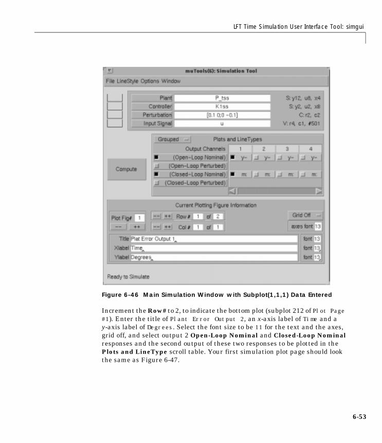
LFT Time Simulation User Interface Tool: simgui
Figure 6-46 Main Simulation Window with Subplot(1,1,1) Data Entered
Increment the Row# to 2, to indicate the bottom plot (subplot 212 of Plot Page #1). Enter the title of Plant Error Output 2, an x-axis label of Time and ay-axis label of Degrees. Select the font size to be 11 for the text and the axes,grid off, and select output 2 Open-Loop Nominal and Closed-Loop Nominalresponses and the second output of these two responses to be plotted in thePlots and LineType scroll table. Your first simulation plot page should lookthe same as Figure 6-47.
6-53

6 Graphical User Interface Tools
6-5
Figure 6-47 First Simulation Plot Page
Increment the Plot Fig# to 2. This creates a new page with one plot axes andbrings it to the foreground. The Window pull-down menu in any simguiwindow shows all the current simgui windows and allows you to hide thecurrent window or bring any of the other windows to the foreground. For Plot Fig# 2, enter the title of Closed-loop plant outputs and controls, an x-axislabel of Time and a y-axis label of Degrees - Newtons. Select the font size to be9 for the title, and 10 for all the text and the axes, grid off, and select theClosed-Loop Nominal responses. Change the Grouped button in the Plotsand LineType scroll table to Free Form and select the y and u and outputs 3,4, 5 and 6 be plotted. Change the line types of the output 3 to be white, solid(w-), output 4 to be white, dashed (w--), output 5 to be white, dashed-dotted(w-.), and output to be white, dotted (w:). You have now finished setting up theplotting data and labeling the plots. Its now time to calculate thecontinuous-time simulation.
4

LFT Time Simulation User Interface Tool: simgui
Pull down the Window menu from any simgui window and select theParameters window. Select an integration time of 0.01 seconds by entering0.01 into the Integration Step Size editable text, as seen in Figure 6-48.
Figure 6-48 Simulation Parameter Window
Pull down the Window menu in the Parameter window and hide theParameter window. Press the Compute button in the main window to initiatethe simulations. Immediately the message Computing appears in the messagebar and the label on the Compute button changes to Stop. By pressing theStop button, the time simulation will terminate at the next available executionof a break. After the Computing message appears in the message bar, andassuming that the Stop button was not pressed, one of two pieces ofinformation will appear in the message bar. If each simulation is estimated totake less than 3 minutes to compute then a running tab of simulation as itprogresses is shown. If a simulation is estimated to take more than threeminutes to compute the message:
Simulation will take approx. X seconds: check Integration Step Size
6-55

6 Graphical User Interface Tools
6-5
appears in the message bar. The variable X is an estimate of the number ofseconds it will take to calculate the given time simulation. After one second thischanges into a running tab of simulation as it progresses.
Each time simulation in this example should take less than three minutes eachto calculate unless the default Integration Step Size was selected. The resultsof these simulations are shown in Figure 6-49. Note that the time simulationsare calculated for all of the system outputs. Therefore other outputs, notinitially selected, can be displayed by selecting their respective checkboxwithout having to resimulate the system. Similarly outputs can be deselectedwithout deleting them. You should try to select other outputs, change the colorand linetype of the plotted lines, and simulate the open-loop and closed-loopperturbed systems.
6
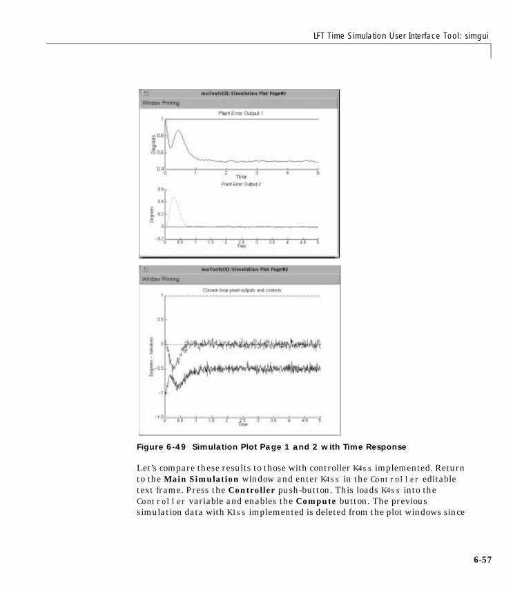
LFT Time Simulation User Interface Tool: simgui
Figure 6-49 Simulation Plot Page 1 and 2 with Time Response
Let’s compare these results to those with controller K4ss implemented. Returnto the Main Simulation window and enter K4ss in the Controller editabletext frame. Press the Controller push-button. This loads K4ss into theController variable and enables the Compute button. The previoussimulation data with K1ss implemented is deleted from the plot windows since
6-57

6 Graphical User Interface Tools
6-5
it is no longer current. Simulate the open-loop and closed-loop nominal systemsby pressing the Compute button. The time responses are shown in Figure 6-50.Comparing this response to the response of K1ss (Figure 6-49), you can see theimproved performance with K4ss implemented.
Figure 6-50 Simulation Plot Page 1 and 2 with Time Response
8

LFT Time Simulation User Interface Tool: simgui
Printing MenuEach Simulation Plot Page has a Printing menu for sending that figure to aprinter or saving it to a file. Selecting the Print option from the Printing menuwill pop up a Print dialog box, as shown in Figure 6-51. This window has threeeditable text boxes across from Device, Options, and Filename, and a Printand Cancel button. The Device, Options, and Filename correspond to theexact same inputs you would provide to the standard MATLAB printcommand. Therefore, the exact string -dps and a filename have to be enteredinto the Device and Filename editable text respectively, to output the plot toa postscript file.
Leaving the three editable text boxes empty and pressing the Print button willsend the current figure to the printer. This is similar to the MATLAB printcommand. Pressing the Cancel button will not execute any print command.After filling in any or all of the three editable text boxes, pressing the Printbutton will execute the MATLAB print command. Pressing either Print orCancel executes that command and hides this window.
Figure 6-51 Printing Dialog Box
Loading and Saving Plot InformationThe File menu of the main simulation window contains a Load Setup, Save Setup, and Quit as seen in Figure 6-52.
Figure 6-52 File Pull-down Menu
6-59

6 Graphical User Interface Tools
6-6
Selecting the Load Setup from the menu will pop up a Load Setup dialog box,as shown in Figure 6-53. The Load Setup option is used to load plot setupinformation that was previously saved using the Save Setup option. You canenter a Variable name, (the default is SAVESET), and a Filename. If theFilename editable text is left empty, the variable is loaded from the currentworkspace. Pressing the Load button loads the data from the locationdescribed by the Variable and Filename data and hides the window. PressingCancel hides the window and loads no data. The data loaded includes all thePlots and LineTypes Table information, plotting information and labels, finaltime, integration time, sample time, initial conditions, export suffix, andsimulation name if available. If an error occurs during the load operation, anerror message will appear in the main window message bar.
Selecting Save Setup from the File menu will pop up a Save Setup dialog box,very similar to Figure 6-53 except with the Save button replacing the Loadbutton. This option saves all the current plot and line type data along with thelabels, final time, integration time, sample time, initial conditions, exportsuffix, and simulation name, if available, to the Variable string name.
The Variable and Filename editable text and the Cancel button operate in theexact same manner as in the Load Setting dialog box. Pressing the Savebutton saves the data to the current workspace in the Variable editable textstring. If this is empty, the default variable name is set to SAVESET. The data issaved to the filename defined by the Filename editable text, or to the filenameSAVESET if there is no Filename string.
The Load Setup and Save Setup options are extremely useful. They allow youto customize simulation plots for use with many plants, controllers,perturbations, and input signals.
The Quit button of the File menu exits the simgui tool and deletes all the dataand windows opened by simgui.
Figure 6-53 Load Setup Dialog Box
0

LFT Time Simulation User Interface Tool: simgui
Simulation TypeYou can select three different time simulations from the Options menu on themain window, as seen in Figure 6-54.
Figure 6-54 Options Pull-down Menu
The default is continuous-time simulation which assumes that the Plant,Controller, and Perturbation variables are either continuous-timeSYSTEMs, CONSTANTs, or not entered. Continuous-time simulations areperformed using the trsp command and make use of the Final Time andIntegration Step Size if you have input them in the Parameter window. Thedefault final time is the last time data in the Input Signal. An integration stepsize is calculated by trsp if you do not provided one. See trsp for moreinformation.
Note: The trsp command is conservative in its selection of an integrationtime; therefore, not inputting an Integration Step Size may lead to verytime-consuming simulations!
Discrete-time simulations assume that the Plant, Controller, andPerturbation variables are either discrete-time SYSTEMs with the samesample rate, CONSTANTs, or not entered. Discrete-time simulations areperformed using the dtrsp command and make use of the Final Time andSample Time if you input them in the Parameter window. The default finaltime is the last time data in the Input Signal. The default sample time is 1.See dtrsp for more information.
A sample-data time simulation assumes that the Plant and Perturbationvariables are either continuous-time SYSTEMs or CONSTANTs. TheController variable is assumed to be either a discrete-time SYSTEM,CONSTANT, or not entered. Sample-data time simulations are performedusing the sdtrsp command and make use of the Final Time, Integration Step Size and Sample Time if you input them in the Parameter window. The
6-61

6 Graphical User Interface Tools
6-6
default final time and integration step size are the same as in thecontinuous-time case. The default sample time is the same as the discrete-timecase, 1. See sdtrsp for more information.
Progress of all these simulations is shown in the message bar of the mainwindow during their computation.
Simulation Parameter WindowThe initial Parameter window is shown in Figure 6-48. The Simulation Dataframe contains data that is used in the calculation of the time responses. TheFinal Time data is used by all the simulations to define the final simulationtime and overrides the final time of the Input Signal data. The default, anempty Final Time editable text string, is the final time of the Input Signaldata. The Integration Step Size data defines the integration step size usedby the continuous and sampled-data simulations. The default, an emptyIntegration Step Size editable text string, is to have the trsp calculate theintegration step size. The Sampled Time is the sample rate used by thediscrete-time and sampled-data simulations. The default Sampled Time is 1.All three variables must be positive, nonzero numbers.
Note that all the variables with editable text to the right of them are encasedin < >. This notation denotes that these variables are optional and are notrequired. The simgui program either calculates the value, Final Time andIntegration Step Size, or assigns them a default value.
The Plant open-loop plant, Controller, and Perturbation initial conditionsmay be entered in their respective editable text boxes. These must be a single,real column vector whose size is the same as the number of states of therespective variable. You can input any workspace variable or valid MATLABexpression to define the initial conditions. The default, with the editable textboxes left empty, is for all the initial conditions to be zero. Incorrect initialcondition data will result in an error message in the main window message bar.
The second column of data in the Parameter window corresponds to theExport Suffix, Simulation Tool Name and the linkable variables frame.Export Suffix is used for data that is automatically exported to the MATLABworkspace upon computation. This string is appended to default names for thevariables as they are exported to the workspace. The Simulation Tool Namemodifies the title of each simgui figure. The linkable variable frame contains alist of simgui variables that can be dragged, using the mouse button, to otherµ-Tools user interface tools. Table 6-2 contains a list of the linkable variables
2

LFT Time Simulation User Interface Tool: simgui
and their meaning. See “Dragging and Dropping Icons” for more informationon how to drag and drop µ-Tools linkage variables.
Table 6-2 Linkable Variables for simgui
The Export to Workspace frame contains variables that you can export to theMATLAB workspace. Each variable is a radio button, which you can select ordeselect. If a variable is selected, the variable is exported to the MATLABworkspace each time that simulation is performed. The default setting is toexport YOLN, YOLP, YCLN, and YCLP every time they are calculated. The Exportto Workspace names and variables are:
• Open-Loop Nominal time response, YOLN.
• Open-Loop Perturbed time response, YOLP.
• Closed-Loop Nominal time response, YCLN.
• Closed-Loop Perturbed time response, YCLP.
• Plant, the open-loop interconnection SYSTEM.
• Controller
• Perturbation
• Input Signal
Linkable Variable Meaning
Plant Open-loop interconnection SYSTEM
K The Controller variable
Pert The Perturbation variable
Input The Input Signal variable
YOLN Open-Loop Nominal time response
YOLP Open-Loop Perturbed time response
YCLN Closed-Loop Nominal time response
YCLP Closed-Loop Perturbed time response
6-63

6 Graphical User Interface Tools
6-6
The Iteration Suffix string is appended to the end of all the output variablesselected. The default is to export the time simulation data YOLN, YOLP, YCLN,and YCLP as they are computed.
Note: These exported variables are overwritten with their new outputresponses after the individual time responses are calculated.
Returning to the example, press the Refresh Variables button in theWorkspace Manager if it is currently open. We can see from the WorkspaceManager that the open-loop nominal time response, YOLN, and the closed-loopnominal time response, YCLN, are saved in the MATLAB workspace (see Figure6-56). This is based on the setting of the Export to Workspace radio buttons.YOLP and YCLP are not in the MATLAB workspace since the open-loop andclosed-loop perturbed responses were not calculated in this example.
4
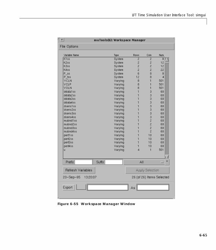
LFT Time Simulation User Interface Tool: simgui
Figure 6-55 Workspace Manager Window
6-65

6 Graphical User Interface Tools
6-6
Dragging and Dropping IconsAll the µ-Tools graphical user interface (GUI) programs, wsgui, dkitgui, andsimgui have a drag and drop facility. The data icons that can be dragged comefrom a scroll table of linkable variable names in each program. In wsgui, theMATLAB workspace variable names currently in the main scroll table (seeFigure 6-57) are the icons that are dragable. In dkitgui, the scroll table shownin Figure 6-56 contains the linkable variable names that are dragable. Thesimgui scroll table shown in Figure 6-56 contains the variables from simguithat are dragable. The left column shows the names of the link variables andthe right column describes their meaning.
Figure 6-56 dkitgui (left) and smgui (right) Linkable Variables Icon Tables for Dragging
To drag an icon, which is a variable name, position the mouse arrow over thevariable name to be dragged. Press the left mouse button and hold the buttondown. You have now selected the variable name for dragging. For example,select the idmod variable for dragging from the wsgui scroll table and move themouse button slightly. (Note: the wsgui workspace has just loaded the mk_wtsfile from the MATLAB workspace.) Your screen should look similar to Figure6-57.
6

Dragging and Dropping Icons
Figure 6-57 Dragging the Controller Variable Name in dkitgui
There are several important facts regarding the dragging and dropping of iconsthat should be noted:
• Icons being dragged are only visible in windows, and they are not visiblewhen the icons are over a frame or other MATLAB uicontrol objects.
• Dragging an icon may be slow on networked computers. This is due to theoverhead of transferring the information about the icon being dragged.
• The drag and drop operation is only completed if the icon is deposited in adrop box.
6-67

6 Graphical User Interface Tools
6-6
Items being dragged need to be deposited directly inside a drop box. Anexample of a drop box is shown in Figure 6-59; it’s to the left of the Controllerpush-button in the simgui main window. To do this, position the icon beingdragged in the center of a drop box and release the mouse button.
Figure 6-58 Drag Khinf from dkitgui to simgui
For example, you can select to drag the fourth D – K iteration controller fromthe spinning satellite example in the “D-K Iteration User Interface Tool:dkitgui” section to the LFT time simulation tool, simgui. Select the Khinf linkvariable in the dkitgui main window and move the mouse button slightly(Figure 6-57). Drag the Khinf link variable over to the main simgui window(Figure 6-58) and drop it in the Controller drop box, as shown in Figure 6-59.Upon successfully dragging and dropping the data, the stringgrabvar(1,’Khinf’) appears in the main simgui window Controller editabletext frame.
8

Dragging and Dropping Icons
Figure 6-59 Drop Khinf into simgui Controller Drop Box
6-69
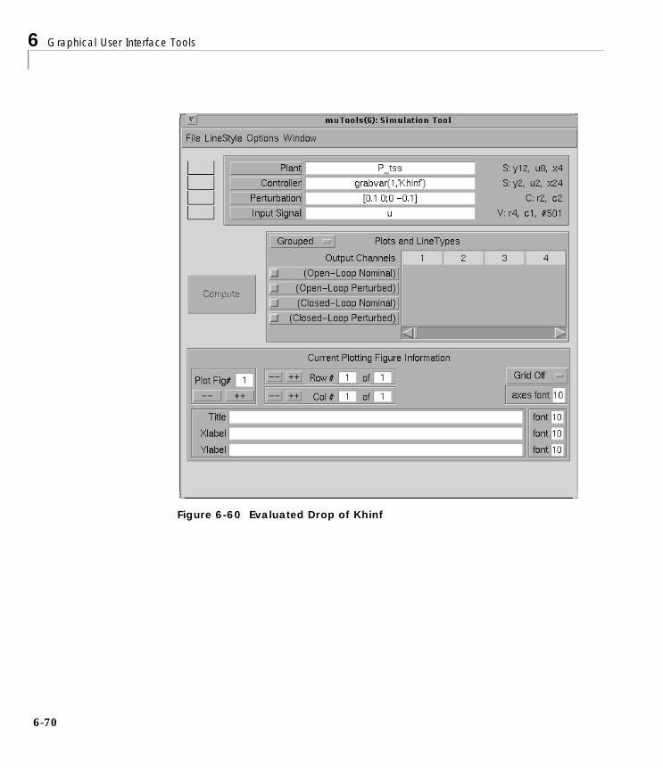
6 Graphical User Interface Tools
6-7
Figure 6-60 Evaluated Drop of Khinf
0

Dragging and Dropping Icons
In simgui and dkigui the linkable variables are to be extracted from a largestorage matrix. The program grabvar performs this operation. The inputs tothe grabvar function are the µ-Tools GUI figure number and the variable namein the originating function. In this example, the variable dragged from dkitguito simgui is Kinf. The dkitgui figure number is 1, which corresponds to the 1in the simgui editable text: grabvar(1,’Khinf’), as seen in Figure 6-60. Thedrag and drop operation is responsible for entering the required input data andrequires no additional input from you.
6-71

6 Graphical User Interface Tools
6-7
2
7
Robust Control Examples
7 Robust Control Examples
7-2
This chapter has a number of examples to show how to apply the µ-Analysisand Synthesis Toolbox (µ-Tools) to robust control problems. These examplesinclude:
• SISO Gain and Phase Margins
• MIMO Loop-at-a-Time Margins
• Analysis of Controllers for an Unstable System
• MIMO Margins Using µ• Space Shuttle Robustness Analysis
• HIMAT Robust Performance Design Example
• F–14 Lateral-directional Control Design
• A Process Control Example: Two Tank System

SISO Gain and Phase Margins
SISO Gain and Phase MarginsGain and phase margins play an important role in control by definingrobustness margins for systems. Unfortunately these margins, by themselves,may be misleading in some cases.
Consider the plant
G = nd2sys([1 –2],[2 –1],–1);minfo(G)
and four different controllers that stabilize the plant
Construct the controller K1 and form the closed-loop using formloop.
k1 = 1;T1 = formloop(G,k1,'neg','pos');spoles(T1)
The command formloop produces a 2-input, 2-output system T1, as shown inFigure 7-1. The third input argument 'neg' denotes that there is negativefeedback on the y2 channel. The fourth input argument 'pos' denotes that thefeedback forward input u2 is positive. These are the default values forformloop.
G s( ) s 2–2s 1–---------------=
K1 s( ) 1=
K2 s( ) s β+βs 1+---------------- β 0 as,> β 2→( )=
K3 s( ) βs 1+s β+
---------------- β 0 as,> β 2→( )=
K4 s( ) s 2.5+2.5s 1+---------------------
1.7s2 1.5s 1+ +
s2
1.5s 1.7+ +-----------------------------------------=
7-3

7 Robust Control Examples
7-4
Figure 7-1 formloop Interconnection Structure
For the problem at hand, form the closed-loop system and calculate the poles ofthe closed-loop system.
K2 = nd2sys([1 1.9],[1.9 1]);clp2 = formloop(G,K2);spoles(clp2)k3 = nd2sys([1.9 1],[1 1.9]);clp3 = formloop(G,k3);spoles(clp3) k4 = nd2sys([1 2.5],[2.5 1]);k4 = mmult(k4,nd2sys([1.7 1.5 1],[1 1.5 1.7]));clp4 = formloop(G,k4);spoles(clp4)
For gain and phase margins, we are interested in the loop transfer functionL(s) := G(s) K(s). Select a frequency range of 0.01 rad/sec to 100 rad/sec with100 points. Calculate the frequency response of the loop transfer function andplot the Bode and Nyquist diagrams of L. The command add_disk adds a unitdisk to the Nyquist plot. The results are shown in Figure 7-2.
omega = logspace(–2,2,100);G_g = frsp(G,omega);k1_g = frsp(k1,omega);L1 = mmult(G_g,k1_g);K2_g = frsp(K2,omega);L2 = mmult(G_g,K2_g);k3_g = frsp(k3,omega);L3 = mmult(G_g,k3_g);k4_g = frsp(k4,omega);L4 = mmult(G_g,k4_g);vplot('nyq',L1,'-',L2,'--',L3,'-.',L4,'.'), add_diskaxis([–4 1 –1 1])vplot('bode',L1,'-',L2,'--',L3,'-.',L4,'.'), grid
u1
u2
y1
y2
T u1 y1
u2
y2
+
+
+- - - - -
?K Gg g
6

SISO Gain and Phase Margins
Controller K1 provides a compromise between a large gain and phase margin.Controller K2 optimizes the gain margin for this example, whereas controllerK3 optimizes the phase margin. Controller K4 tries to optimize both gain andphase margins, resulting with about 50° phase margin, and a gain margin of 3(it can tolerate increase or decrease in gain by a factor of 3). These margins,though, are very sensitive to small changes in the plant (a 50% gain change, toeither 1.5 or 0.67, reduces the phase margin to less than 10°) illustrating thatgain and phase margins are not always an accurate measure of the robustnessof a control design even for single-input/single-output systems.
7-5

7 Robust Control Examples
7-6
Figure 7-2 Nyquist and Bode Plots of the Loop Gain with k1, k2, k3, and k4
4 3.5 3 2.5 2 1.5 1 0.5 0 0.5 11
0.8
0.6
0.4
0.2
0
0.2
0.4
0.6
0.8
1
Real
Imag
inar
y
Nyquist Plot
102
101
100
101
102
200
150
100
Pha
se (
degr
ees)
Frequency (radians/sec)
102
101
100
101
102
101
100
101
Log
Mag
nitu
de
Frequency (radians/sec)
Bode Plot
k1 (solid line) k2 (dashed line) k3 (dash-dotted line) k4 (dotted line)

MIMO Loop-at-a-Time Margins
MIMO Loop-at-a-Time MarginsThis example is designed to illustrate that loop-at-a-time margins (gain, phase,and/or distance to –1) can be inaccurate measures of multivariable robustnessmargins. We will see that margins of the individual loops may be very sensitiveto small perturbations within other loops.
The nominal closed-loop system considered here is shown in Figure 7-3.
Figure 7-3 Nominal Closed-Loop System
G and K are 2 × 2 multi-input/multi-output (MIMO) systems, defined as
Set α := 10, construct G in state-space form and compute its frequencyresponse.
a = [0 10;–10 0];b = eye(2);c = [1 10;–10 1];G = pck(a,b,c);K = eye(2);omega = logspace(–3,2,50);Gg = frsp(G,omega);minfo(Gg);
We want to consider perturbations to both input channels, as shown in Figure7-4.
K G
d - -
6 -d -6
G := 1
s2 α2+
------------------ s α2– α s 1+( )
α– s 1+( ) s α2–
K I2=,
7-7
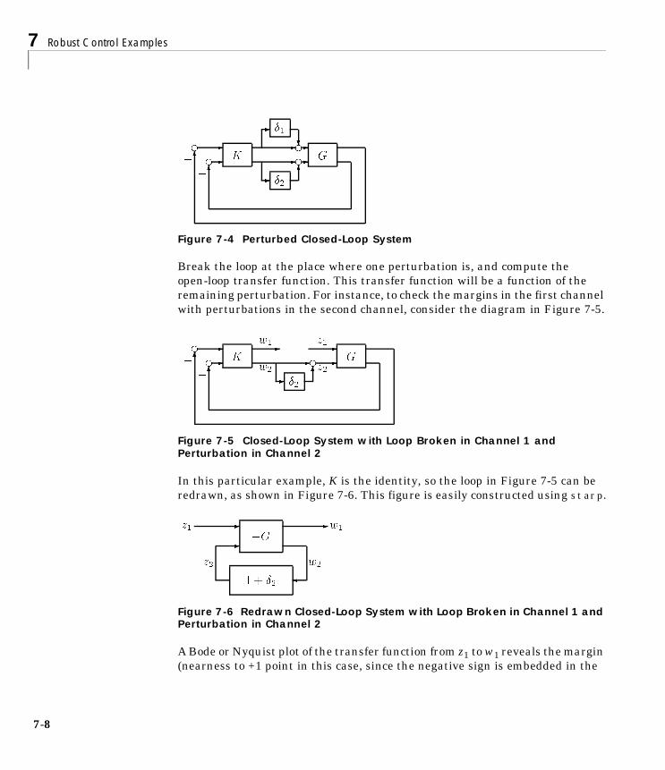
7 Robust Control Examples
7-8
Figure 7-4 Perturbed Closed-Loop System
Break the loop at the place where one perturbation is, and compute theopen-loop transfer function. This transfer function will be a function of theremaining perturbation. For instance, to check the margins in the first channelwith perturbations in the second channel, consider the diagram in Figure 7-5.
Figure 7-5 Closed-Loop System with Loop Broken in Channel 1 and Perturbation in Channel 2
In this particular example, K is the identity, so the loop in Figure 7-5 can beredrawn, as shown in Figure 7-6. This figure is easily constructed using starp.
Figure 7-6 Redrawn Closed-Loop System with Loop Broken in Channel 1 and Perturbation in Channel 2
A Bode or Nyquist plot of the transfer function from z1 to w1 reveals the margin(nearness to +1 point in this case, since the negative sign is embedded in the
K G
d - - d-
- 1
?
- 66 -d - d-
26
K G
z1w1
z2w2
d - - -
6 -d - d -
2- 66

MIMO Loop-at-a-Time Margins
transfer function from z to w) in the first channel as a function of perturbationsin the second channel. Refer to Figure 7-6 and calculate the nominal transferfunction obtained by breaking the loop in the 1st channel. A Bode plot of thetransfer function is shown in Figure 7-7. Note that this loop is an integrator, sothe single-loop margin is great. In a similar manner, calculate the nominaltransfer function obtained by breaking the loop in the second channel. Theresults are shown in Figure 7-7.
nom_ch1_lb = starp(mscl(Gg,–1),1,1,1);nom_ch2_lb = starp(1,mscl(Gg,–1),1,1);vplot('bode',nom_ch1_lb,'-',nom_ch2_lb,'--');
Figure 7-7 Bode Plot the Single-Loop Transfer Functions
The previous Bode plots show that each channel can tolerate large,loop-at-a-time, gain variations. Now though, consider a simultaneous 10%variation in each loop. Specifically, check the internal stability of the perturbedclosed-loop shown in Figure 7-4, redrawn in Figure 7-8, with ,and .
103
102
101
100
101
102
0
100
Pha
se (
degr
ees)
Frequency (radians/sec)
103
102
101
100
101
102
102
100
102
104
Log
Mag
nitu
de
Frequency (radians/sec)
Bode Plot: Single Loop Broken in Channel 1 and 2
δ1 1– 101⁄=δ2 1 101⁄=
7-9
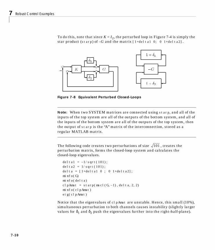
7 Robust Control Examples
7-1
To do this, note that since K = I2, the perturbed loop in Figure 7-4 is simply thestar product (starp) of –G and the matrix [1+delta1 0; 0 1+delta2].
Figure 7-8 Equivalent Perturbed Closed-Loops
Note: When two SYSTEM matrices are connected using starp, and all of theinputs of the top system are all of the outputs of the bottom system, and all ofthe inputs of the bottom system are all of the outputs of the top system, thenthe output of starp is the “A” matrix of the interconnection, stored as aregular MATLAB matrix.
The following code creates two perturbations of size , creates theperturbation matrix, forms the closed-loop system and calculates theclosed-loop eigenvalues.
delta1 = –1/sqrt(101);delta2 = 1/sqrt(101);delta = [1+delta1 0 ; 0 1+delta2];minfo(G)minfo(delta)clpAmat = starp(mscl(G,–1),delta,2,2)minfo(clpAmat)eig(clpAmat)
Notice that the eigenvalues of clpAmat are unstable. Hence, this small (10%),simultaneous perturbation to both channels causes instability (slightly largervalues for δ1 and δ2 push the eigenvalues further into the right-half-plane).
101
0

MIMO Loop-at-a-Time Margins
We can see the effect of simultaneous perturbations with the help of a Nyquistplot. Refer back to Figure 7-6 and calculate the transfer function obtained bybreaking the loop in the first channel, with a perturbation of δ2 = 0.001. Thesingle-loop margin in channel 1 is still quite large, since the Nyquist plot, solidline in Figure 7-9 intersects the real axis around 11. Try a slightly larger valuefor δ2 (again, note that the +1 point is of interest due to the extra minus (–) signon G).
delta2 = 0.001;pert_ch1_lb1 = starp(mscl(Gg,–1),1+delta2,1,1);vplot('nyq',pert_ch1_lb1);delta2 = 0.01;pert_ch1_lb2 = starp(mscl(Gg,–1),1+delta2,1,1);vplot('nyq',pert_ch1_lb1,'-',pert_ch1_lb2,'--');add_disk
Note the significant degradation in the margin due to a 1% variation inchannel 2.
Figure 7-9 Nyquist Plot of Simultaneously Perturbed Closed-Loop System
2 0 2 4 6 8 10 121
0
1
2
3
4
5
6Nyquist Plot: Loop Broken in Channel 1, Delta2 =.001, .01
Real
Imag
inar
y
unit disk (solid) δ2 = 0.001 (solid) δ2 = 0.01 (dashed)
7-11

7 Robust Control Examples
7-1
It is easy to write a for loop (as in ex_ml1) that calculates the open-loopfrequency response in channel 1 for several values of δ2. Six δ2 values areconstructed from 0.001 to 0.1. A for loop calculates the perturbed loop transferfunction in channel 1 for the six values of δ2 and their responses are plotted ona Nyquist diagram.
file:ex_ml1.mdelta2values = logspace(–3,–1,6);pert_ch1_lb = [];for i=1:length(delta2values)
delta2 = delta2values(i);pert_ch1_lb = ...sbs(pert_ch1_lb,starp(mscl(Gg,–1),1+delta2,1,1));
endxa = vpck([–2; 12],[1 2]);ya = vpck([-sqrt(–1); 6*sqrt(–1)],[1 2]);vplot('nyq',pert_ch1_lb,xa,ya);title('Loop Broken in Channel 1, Delta2 in [.001 .1]')xlabel('Real')ylabel('Imag')
Typing
ex_ml1
at the command line generates Figure 7-10. Note that the margin in channel 1rapidly disappears due to small perturbations in channel 2.
2
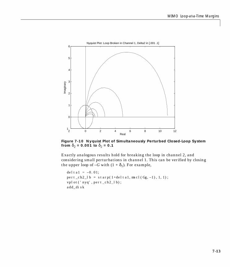
MIMO Loop-at-a-Time Margins
Figure 7-10 Nyquist Plot of Simultaneously Perturbed Closed-Loop System from δ2 = 0.001 to δ2 = 0.1
Exactly analogous results hold for breaking the loop in channel 2, andconsidering small perturbations in channel 1. This can be verified by closingthe upper loop of –G with (1 + δ1). For example,
delta1 = –0.01;pert_ch2_lb = starp(1+delta1,mscl(Gg,–1),1,1);vplot('nyq',pert_ch2_lb);add_disk
2 0 2 4 6 8 10 121
0
1
2
3
4
5
6Nyquist Plot: Loop Broken in Channel 1, Delta2 in [.001 .1]
Real
Imag
inar
y
7-13

7 Robust Control Examples
7-1
Figure 7-11 Nyquist Plot of Simultaneously Perturbed Closed-Loop System for δ1 = –0.01
Hence, in a multivariable system the single loop margins may be good thoughsimultaneous interaction of perturbations in each loop may lead to instability,even for small perturbations. The structured singular value, µ, can be used todetect the nonrobustness in this feedback system. To see this we will reanalyzethis example using µ in the “MIMO Margins Using µ” section in this chapter.
2 1.5 1 0.5 0 0.5 12
1.5
1
0.5
0
0.5
1
1.5
2Nyquist Plot: Loop Broken in Channel 2, Delta1 = 0.01
Real
Imag
inar
y
4

Analysis of Controllers for an Unstable System
Analysis of Controllers for an Unstable SystemUnstable example Recall from the “Unmodeled Dynamics” section in Chapter4, the example with the nominal plant model
and the multiplicative input uncertainty model
G and Wu describe a set M(G, Wu) of plant models defined by
(7-1)
with the restriction that the number of right-half plane poles of perturbed plantequal the number of right-half plane poles of G. The nominal model G,weighting function Wu, and the unknown transfer function ∆G are used toparameterize all the possible models.
We are interested in the stability and performance of the closed-loop system forall possible plant models in the set M(G, Wu). In this example, we choose theperformance objective to be a stable, closed-loop system, and outputdisturbance rejection up to 0.6 rad/sec, with at least 100:1 disturbance rejectionat DC.
This objective can approximately be represented as a weighted H∞ normconstraint on the sensitivity function,
for all ∈ M(G, Wu), using the weighting function
G :=1
s 1–------------
Wu :=14---
12---s 1+( )
132-------s 1+
----------------------
M G Wu,( ) := G I ∆GWu+( ) : max ∆G jω( ) 1≤ .ω
Wp
1 GK–------------------
∞
1≤
G
7-15

7 Robust Control Examples
7-1
A block diagram of this uncertain closed-loop system illustrating theperformance objective (closed-loop transfer function from d → e) is shown inFigure 7-12.
Figure 7-12 Uncertain Closed-Loop System
Grouping G, Wu, and Wp together (as P), the uncertain closed-loop system isredrawn in Figure 7-13.
Figure 7-13 General Interconnection for Uncertain System
Type
ex_unic
to create the plant model, weighting functions and the open-loopinterconnection P. The commands in ex_unic are as follows:
Wp:=14---s 0.6+
s-------------------- s 0.006+=
- K -u 6
Wu
- G
?- G - g?
d
- Wp- eg
+
+
Plant model set
P
G
K
w
e d
z
y u
-
-
6

Analysis of Controllers for an Unstable System
file: ex_unic.mG = nd2sys(1,[1 –1]);Wu = nd2sys([0.5 1],[0.03125 1],.25);WP = nd2sys([.25 0.6],[1 0.006]);systemnames = 'G Wu WP';
sysoutname = 'P';inputvar = '[ z; d; u ]';input_to_p = '[ z + u ]';input_to_Wu = '[ u ]';input_to_WP = '[ G + d ]';outputvar = '[ Wu; WP; G + d ]';cleanupsysic = 'yes';
sysic
Next, consider two controllers, K1 and K2 which stabilize the nominal plantmodel G.
For each controller, define M := FL(P,K). M22 is the nominal d → e transferfunction, and hence, nominal performance is characterized by ||M22||∞ ≤ 1. Themagnitude of the M22 transfer function with K1 and K2 implemented is shownin Figure 7-14. Both controllers easily achieve the nominal performanceobjective.
M11 is the transfer function that the perturbation ∆ sees, so that robuststability over M(G, Wu) is equivalent to ||M11||∞ < 1. The magnitude of the M11transfer function is shown in Figure 7-15. Both controllers achieve the robuststability objective.
K1 10–0.9s 1+
s--------------------- K2 1–
2.8s 1+s
---------------------==
7-17
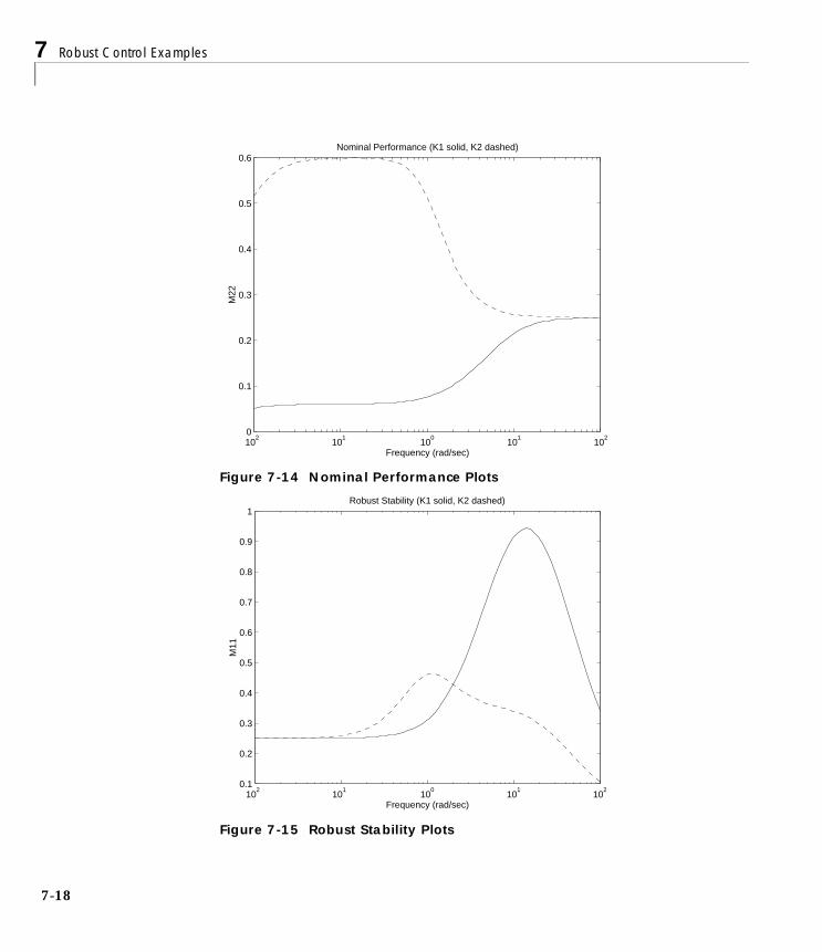
7 Robust Control Examples
7-1
Figure 7-14 Nominal Performance Plots
Figure 7-15 Robust Stability Plots
102
101
100
101
102
0
0.1
0.2
0.3
0.4
0.5
0.6
Frequency (rad/sec)
M22
Nominal Performance (K1 solid, K2 dashed)
102
101
100
101
102
0.1
0.2
0.3
0.4
0.5
0.6
0.7
0.8
0.9
1
Frequency (rad/sec)
M11
Robust Stability (K1 solid, K2 dashed)
8
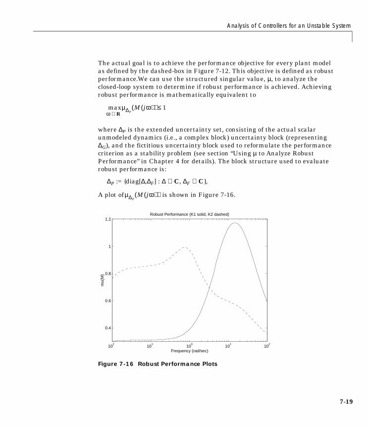
Analysis of Controllers for an Unstable System
The actual goal is to achieve the performance objective for every plant modelas defined by the dashed-box in Figure 7-12. This objective is defined as robustperformance.We can use the structured singular value, µ, to analyze theclosed-loop system to determine if robust performance is achieved. Achievingrobust performance is mathematically equivalent to
where ∆P is the extended uncertainty set, consisting of the actual scalarunmodeled dynamics (i.e., a complex block) uncertainty block (representing∆G), and the fictitious uncertainty block used to reformulate the performancecriterion as a stability problem (see section “Using µ to Analyze RobustPerformance” in Chapter 4 for details). The block structure used to evaluaterobust performance is:
∆P := diag[∆,∆F] : ∆ ∈ C, ∆F ∈ C,
A plot of is shown in Figure 7-16.
Figure 7-16 Robust Performance Plots
maxµ∆PM jω( )( ) 1≤
ω R∈
µ∆PM jω( )( )
102
101
100
101
102
0.4
0.6
0.8
1
1.2
Frequency (rad/sec)
mu(
M)
Robust Performance (K1 solid, K2 dashed)
7-19

7 Robust Control Examples
7-2
Note that while K1 achieves better nominal performance than K2, the closed-loop system with K2 has better robust performance properties than with K1. Infact, the controller K2 does, just barely, achieve robust performance. Hence, forevery plant , the closed-loop system, with K2 is stable, andmoreover
This is not true for the closed-loop system with K1, as the robust performancetest, using µ is not satisfied for FL(P,K1).
The script-file
ex_usrp
constructs the controllers, forms the closed-loop systems, calculates theclosed-loop frequency responses, performs the analysis, and generates theplots. A listing of ex_usrp is as follows:
G M G Wu,( )∈
Wp
1 GK2–---------------------
∞
< 1
0
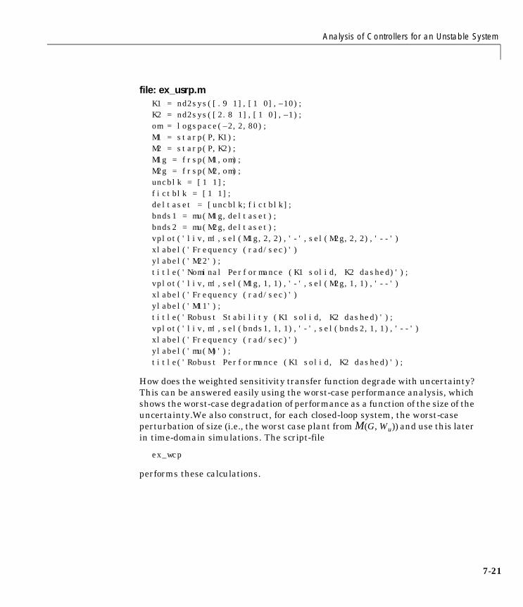
Analysis of Controllers for an Unstable System
file: ex_usrp.mK1 = nd2sys([.9 1],[1 0],–10);K2 = nd2sys([2.8 1],[1 0],–1);om = logspace(–2,2,80);M1 = starp(P,K1);M2 = starp(P,K2);M1g = frsp(M1,om);M2g = frsp(M2,om);uncblk = [1 1];fictblk = [1 1];deltaset = [uncblk;fictblk];bnds1 = mu(M1g,deltaset);bnds2 = mu(M2g,deltaset);vplot('liv,m',sel(M1g,2,2),'-',sel(M2g,2,2),'--')xlabel('Frequency (rad/sec)')ylabel('M22');title('Nominal Performance (K1 solid, K2 dashed)');vplot('liv,m',sel(M1g,1,1),'-',sel(M2g,1,1),'--')xlabel('Frequency (rad/sec)')ylabel('M11');title('Robust Stability (K1 solid, K2 dashed)');vplot('liv,m',sel(bnds1,1,1),'-',sel(bnds2,1,1),'--')xlabel('Frequency (rad/sec)')ylabel('mu(M)');title('Robust Performance (K1 solid, K2 dashed)');
How does the weighted sensitivity transfer function degrade with uncertainty?This can be answered easily using the worst-case performance analysis, whichshows the worst-case degradation of performance as a function of the size of theuncertainty.We also construct, for each closed-loop system, the worst-caseperturbation of size (i.e., the worst case plant from M(G, Wu)) and use this laterin time-domain simulations. The script-file
ex_wcp
performs these calculations.
7-21

7 Robust Control Examples
7-2
file: ex_wcp.m[deltabad1,wcp_l1,wcp_u1] = wcperf(M1g,uncblk,1,8);[deltabad2,wcp_l2,wcp_u2] = wcperf(M2g,uncblk,1,8);vplot(wcp_l1,wcp_u1,wcp_l2,'--',wcp_u2,'--')xlabel('Size of Delta_G')ylabel('Weighted Sensitivity')title('Performance Degradation (K1 solid, K2 dashed)')
The performance degradation curve is shown in Figure 7-17. The fourthargument to wcperf, in this case 8, means that there will be at least 8 pointsin the performance degradation curve.
Figure 7-17 Performance Degradation
This clearly shows that for perturbations ∆G satisfying
0 0.2 0.4 0.6 0.8 1 1.2 1.4 1.6 1.80
0.5
1
1.5
2
2.5
3
3.5
Size of Delta_G
Wei
ghte
d S
ensi
tivity
Performance Degradation (K1 solid, K2 dashed)
k1 (solid line) k2 (dashed line)
max ∆G jω( ) Š 0.76,ω
2

Analysis of Controllers for an Unstable System
the robust closed-loop performance using K2 is better than that obtained usingK1. The perturbations deltabad1 and deltabad2 are the worst-caseperturbations ∆G, of size 1.They each cause the weighted sensitivity to degradea maximal amount, over all perturbations of size 1. In the case of K1, theperturbation deltabad1 causes the weighted sensitivity to degrade toapproximately 3.5, while in the case of K2, deltabad2 causes the weightedsensitivity to degrade to approximately 1.0. We will use these worst-caseperturbations in time-domain simulations.
Based on the robust performance analysis results, K2 will stabilize the nominalplant and the seven extreme plant models discussed in the “UnmodeledDynamics” section in Chapter 4. Also, the performance degradation, in termsof the weighted sensitivity function, should be small. Using controller K1,stability is also guaranteed. However, since FL(P,K1)(jω) has a peak µ-value ofabout 1.2, it is clear that K1 does not have robust performance over the setM(G,Wu) and we expect the performance degradation over the seven extremeplants to be worse than that using K2.
These seven plants, all of which are members of the set M(G,Wu) and theworst-case plant from M(G,Wu), are
and are constructed via
ex_mkpl
The contents of ex_mkpl are listed below.
Gwc G 1 ∆wcWu+( )[ ]=
G51
s 1–------------
702
s2 2 0.15 70s 702+⋅ ⋅+
-------------------------------------------------------------
=
G71
s 1–------------
50s 50+---------------
=6
G61
s 1–------------
702
s2 2 5.6 70s 702+⋅ ⋅+
----------------------------------------------------------
=
G11
s 1–------------
6.1s 6.1+-----------------
= G21.425
s 1.425–-----------------------=
G3.67
s 0.67–--------------------= G4
1s 1–------------
0.07s– 1+0.07s 1+
---------------------------- =
7-23
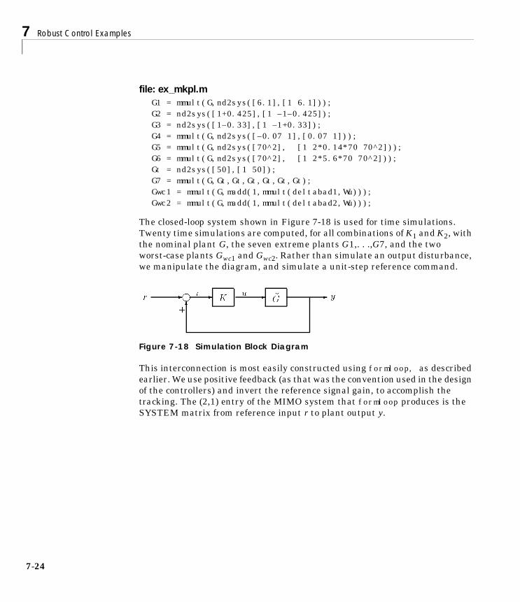
7 Robust Control Examples
7-2
file: ex_mkpl.mG1 = mmult(G,nd2sys([6.1],[1 6.1]));G2 = nd2sys([1+0.425],[1 –1–0.425]);G3 = nd2sys([1–0.33],[1 –1+0.33]);G4 = mmult(G,nd2sys([–0.07 1],[0.07 1]));G5 = mmult(G,nd2sys([70^2], [1 2*0.14*70 70^2]));G6 = mmult(G,nd2sys([70^2], [1 2*5.6*70 70^2]));Gt = nd2sys([50],[1 50]);G7 = mmult(G,Gt,Gt,Gt,Gt,Gt,Gt);Gwc1 = mmult(G,madd(1,mmult(deltabad1,Wu)));Gwc2 = mmult(G,madd(1,mmult(deltabad2,Wu)));
The closed-loop system shown in Figure 7-18 is used for time simulations.Twenty time simulations are computed, for all combinations of K1 and K2, withthe nominal plant G, the seven extreme plants G1,. . .,G7, and the twoworst-case plants Gwc1 and Gwc2. Rather than simulate an output disturbance,we manipulate the diagram, and simulate a unit-step reference command.
Figure 7-18 Simulation Block Diagram
This interconnection is most easily constructed using formloop, as describedearlier. We use positive feedback (as that was the convention used in the designof the controllers) and invert the reference signal gain, to accomplish thetracking. The (2,1) entry of the MIMO system that formloop produces is theSYSTEM matrix from reference input r to plant output y.
4

Analysis of Controllers for an Unstable System
Typing
ex_mkclp
forms the 20 SISO systems, as below:
file: ex_mkclp.mclpg_k1 = sel(formloop(G,K1,'pos','neg'),2,1);clpg1_k1 = sel(formloop(G1,K1,'pos','neg'),2,1);clpg2_k1 = sel(formloop(G2,K1,'pos','neg'),2,1);clpg3_k1 = sel(formloop(G3,K1,'pos','neg'),2,1);clpg4_k1 = sel(formloop(G4,K1,'pos','neg'),2,1);clpg5_k1 = sel(formloop(G5,K1,'pos','neg'),2,1);clpg6_k1 = sel(formloop(G6,K1,'pos','neg'),2,1);clpg7_k1 = sel(formloop(G7,K1,'pos','neg'),2,1);clpgwc1_k1 = sel(formloop(Gwc1,K1,'pos','neg'),2,1);clpgwc2_k1 = sel(formloop(Gwc2,K1,'pos','neg'),2,1);clpg_K2 = sel(formloop(G,K2,'pos','neg'),2,1);clpg1_K2 = sel(formloop(G1,K2,'pos','neg'),2,1);clpg2_K2 = sel(formloop(G2,K2,'pos','neg'),2,1);clpg3_K2 = sel(formloop(G3,K2,'pos','neg'),2,1);clpg4_K2 = sel(formloop(G4,K2,'pos','neg'),2,1);clpg5_K2 = sel(formloop(G5,K2,'pos','neg'),2,1);clpg6_K2 = sel(formloop(G6,K2,'pos','neg'),2,1);clpg7_K2 = sel(formloop(G7,K2,'pos','neg'),2,1);clpgwc1_K2 = sel(formloop(Gwc1,K2,'pos','neg'),2,1);clpgwc2_K2 = sel(formloop(Gwc2,K2,'pos','neg'),2,1);
These closed-loop systems are simulated with a unit-step reference input at t =0.5. The time response with controllers K1 (top) and K2 (bottom) implementedare shown in Figure 7-19.
Typing
ex_ustr
runs the simulations, and generates the time response plots.
7-25

7 Robust Control Examples
7-2
file: ex_ustr.m stepref = step_tr([0 0.5 10],[0 1 1],.01,10);Tfinal = 10;tinc = 0.01;yg_k1 = trsp(clpg_k1,stepref,Tfinal,tinc);yg1_k1 = trsp(clpg1_k1,stepref,Tfinal,tinc);yg7_k1 = trsp(clpg7_k1,stepref,Tfinal,tinc);ygwc1_k1 = trsp(clpgwc1_k1,stepref,Tfinal,tinc);ygwc2_k1 = trsp(clpgwc2_k1,stepref,Tfinal,tinc);yg_k2 = trsp(clpg_k2,stepref,Tfinal,tinc);yg1_k2 = trsp(clpg1_k2,stepref,Tfinal,tinc);ygwc2_k2 = trsp(clpgwc2_k2,stepref,Tfinal,tinc);subplot(211)vplot(vdcmate(yg_k1,5),'+',yg1_k1,yg2_k1, yg3_k1,yg4_k1,...
yg5_k1,yg6_k1,yg7_k1,ygwc1_k1,ygwc2_k1);xlabel('Time (seconds)')title('Closed-loop responses using k1') subplot(212)vplot(vdcmate(yg_k2,5),'+',yg1_k2,yg2_k2, yg3_k2,yg4_k2,...
yg5_k2,yg6_k2,yg7_k2,ygwc1_k2,ygwc2_k2);xlabel('Time (seconds)')title('Closed-loop responses using K2')
Both controllers stabilize all plant models. The closed-loop performanceprovided by K2 is very similar for all the plants. This is expected based on therobust performance analysis using µ, which showed that every plant in the setM(G,Wu) is stabilized and effectively controlled with K2. The closed-loopperformance provided by K1 is not very robust. The large overshoot, undershootand oscillations for some of the responses reinforces the notion that K1 does notachieve robust performance, as defined by the uncertain plant model setM(G,Wu), and the weighted sensitivity transfer function.
6
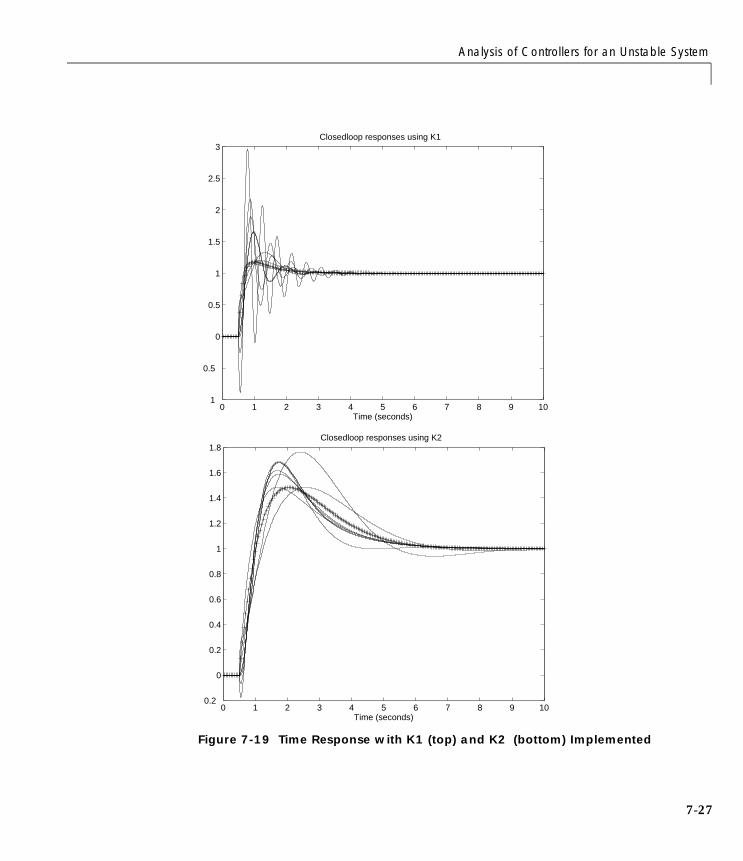
Analysis of Controllers for an Unstable System
Figure 7-19 Time Response with K1 (top) and K2 (bottom) Implemented
0 1 2 3 4 5 6 7 8 9 101
0.5
0
0.5
1
1.5
2
2.5
3
Time (seconds)
Closedloop responses using K1
0 1 2 3 4 5 6 7 8 9 100.2
0
0.2
0.4
0.6
0.8
1
1.2
1.4
1.6
1.8
Time (seconds)
Closedloop responses using K2
7-27

7 Robust Control Examples
7-2
Redesign Controllers Using D – K IterationThe D – K iteration, using dkitgui, can be used to design a robust controllerfor the uncertain plant model M(G,Wu) and weighted sensitivity performanceobjective implied by the interconnection structure in Figure 7-12. Startdkitgui, and enter the data as shown in the dkitgui Setup window, Figure7-20.
Figure 7-20 Unstable System dkitgui Setup Window
Return to the main Iteration window, as shown in Figure 7-21, and pull downthe Iteration menu and select 3 from the Auto Iterate submenu. Figure 7-21shows the main Iteration window after the third iteration has completed.
8

Analysis of Controllers for an Unstable System
Figure 7-21 Main dkitgui Window After Three Iterations
Controller K1dk corresponds to the first D – K iteration H∞ design andcontroller K3dk corresponds to the third D – K iteration design.
Controller K1dk stabilizes all seven plant models, though the performance ispoor, with large settling times, and large overshoot. This is not surprising,based on the robust performance analysis using µ. The value of µ with K1dkimplemented was 1.55(> 1).
Controller K3dk achieves a closed-loop, robust performance µ-value of about0.7, guaranteeing stability and good closed-loop performance for all seven plantmodels (as these are contained in the set M(G,Wu)). The simulations agree withthis conclusion. Note the improvement in overshoot and settling time (andgreater insensitivity) over all of the previous closed-loop simulations (using K1,K2 and K1dk). The nominal responses are denoted by the “+” symbol linetype.Typing
ex_ustrd
generates the plots shown in Figure 7-22.
7-29

7 Robust Control Examples
7-3
Figure 7-22 Time Response with K1dk (top) and K3dk (bottom) Implemented
0 1 2 3 4 5 6 7 8 9 101
0.5
0
0.5
1
1.5
2
2.5
3
Time (seconds)
Closedloop responses using K1
0 1 2 3 4 5 6 7 8 9 100.4
0.2
0
0.2
0.4
0.6
0.8
1
1.2
1.4
1.6
Time (seconds)
Closedloop responses using K3dk
0

Analysis of Controllers for an Unstable System
Near the H∞ optimal solution, the controller tends to have high bandwidth,providing some argument against using the H∞ norm as the sole measure ofperformance. For this reason, we often back off from optimality, leading to alower bandwidth, and more reasonable controller. In the Parameter window,change Gamma Min to 0.78, and change Gamma Max to 0.78. This fixes the nextcontrol design to be at γ = 0.78, which is approximately 10% above the optimalvalue of 0.71. Then, in the Iteration window, press Control Design to produceK4dk. This controller will sacrifice some (about 10%) H∞ performance, but havemuch lower bandwidth. You should repeat the time-domain simulations forthis controller.
You can also do simple model reduction on this controller, using sysbal andstrunc. In the Setup window, type
reducek(
in the <Controller> data entry box. Then, drag, from the Iteration window,the linkable variable Khinf into the Setup window drop box for the controller.Finally, type
,3)
in the controller data entry box, which should now read
reducek(grabvar(2,'Khinf'),3)
The 2 corresponds to the MATLAB figure number associated with theIteration window. In your case, it may not be 2. However, the dragging actionwill put the correct number in this place. Next, press the <Controller>pushbutton. This will grab the current H∞ controller, balance it, and reduce itto third order using a simple M-file reducek, and place the reduced ordercontroller back into Kuse. Kuse is the controller for which all analysis indkitgui takes place (in dkitgui, the variable Kuse is automatically set toKhinf immediately after Khinf is designed). This reenables the Form ClosedLoop pushbutton, which will implement the controller stored in Kuse. Pressingthe Frequency Response and Compute Mu pushbuttons, you can determinethe effectiveness of the reduced order controller, and repeat the process fordifferent choice of controller order. In this example, a third order controller issuitable.
Time responses using this suboptimal, reduced order controller are shown inFigure 7-23.
7-31

7 Robust Control Examples
7-3
Figure 7-23 Time Response with K4dkreduced Implemented
0 1 2 3 4 5 6 7 8 9 100.2
0
0.2
0.4
0.6
0.8
1
1.2
1.4
1.6
1.8
Time (seconds)
Closedloop responses using K4reduced
2

MIMO Margins Using µ
MIMO Margins Using µRecall the conclusions of the “MIMO Loop-at-a-Time Margins” sectionconcerning loop-at-a-time margins in MIMO systems. These margins can beinaccurate measures of multivariable robustness margins. In this exercise, wecompare two controllers for a weighted robust stability problem similar to thatin the“MIMO Loop-at-a-Time Margins” section, and see that the structuredsingular value, µ, accurately predicts their robust stability characteristics.
Consider an uncertainty model consisting of multiplicative uncertainty at theplant input in each channel. A block diagram of the model of the open-loopplant, with perturbations, is shown Figure 7-24.
Figure 7-24 Plant Model with Multiplicative Uncertainty
The linear, time-invariant perturbations, represented by transfer functionsδ1 and δ2, are used to model the uncertainty in the plant, and are assumed tosatisfy
• δi(s) is stable
• ,
but otherwise be unknown. Everything inside the dashed box, in particular, thetransfer functions G, Wδ1 and Wδ2, along with the specific interconnection, areassumed given and known. Since the uncertainty represented by the δi is
G
W2
W1
2
1
u1
u2
c
c
y1
y2
6
z1w1
?
?
?
z2w2
6
6
max δi jω( ) 1<ω R∈
7-33

7 Robust Control Examples
7-3
normalized to 1, the transfer functions Wδi reflect the frequency-dependentsize of the uncertainty.
The first input channel is modeled with 10% uncertainty at low frequency,increasing to 100% uncertainty at approximately 20 rads/sec, and largeruncertainty for higher frequencies. In channel 2, the low frequency uncertaintyis 20%, rising to 100% at approximately 45 rads/sec. Type in the following datafor the problem.
a = [0 10;–10 0];b = eye(2);c = [1 10;–10 1];G = pck(a,b,c);wdel1 = nd2sys([1 2],[1/60 20]);wdel2 = nd2sys([1 9],[1/40 45]);omega = logspace(–3,2,50);wdel1_g = frsp(wdel1,omega);wdel2_g = frsp(wdel2,omega);vplot('liv,lm',wdel1_g,wdel2_g)title('Multiplicative Uncertainty Weights')
Figure 7-25 Multiplicative Uncertainty Weights
101
100
101
102
103
104
101
100
101
102
Multiplicative Uncertainty Weights
Frequency (rad/sec)
Mag
nitu
de
4

MIMO Margins Using µ
To use the µ theory, we need to isolate the perturbations from the knowncomponents. We do this by constructing a four input, four output system, withtwo fictitious input/output pairs (w,z), as well as two actual input/output pairs(u,y). The fictitious inputs and outputs are used to model the multiplicativeuncertainty at the plant input. The system is called P, and is shown below.
The internal structure of P is shown in Figure 7-26.
Figure 7-26 Plant Model with Multiplicative Uncertainty Blocks Pulled Out
The SYSTEM matrix P can be constructed easily from the components, usingthe SYSTEM interconnection program, sysic.
systemnames = 'G wdel1 wdel2';inputvar = '[w2; u2]';input_to_G = '[u(1) + wdel1; u(2) + wdel2]';input_to_wdel1 = '[w(1)]';input_to_wdel2 = '[w(2)]';outputvar = '[u; G]';sysoutname = 'P';sysic;
7-35

7 Robust Control Examples
7-3
The feedback controller for this problem will measure the variables y, andgenerate control signals, u. In a block diagram, the perturbed closed-loopsystem appears as shown in Figure 7-27. In terms of P, the perturbedclosed-loop system appears as Figure 7-28.
Figure 7-27 Closed-Loop System with δ1 and δ2 Uncertainty
Figure 7-28 Closed-Loop System with Uncertainty
Next, we need to construct the transfer function that the 2 × 2 perturbationmatrix ∆ sees, namely M := FL(P,K). This transfer function is computed by
G
W2
W1
2
1
P
K
c
c
6
6
6
z1w1
?
?
?
z2w2
6
6
P
1 0
0 2z1z2
-
w1
w2
K
y1y2
-
u1u2
6
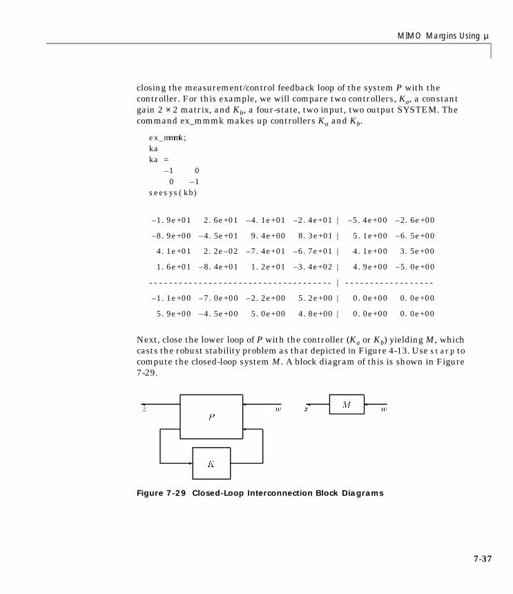
MIMO Margins Using µ
closing the measurement/control feedback loop of the system P with thecontroller. For this example, we will compare two controllers, Ka, a constantgain 2 × 2 matrix, and Kb, a four-state, two input, two output SYSTEM. Thecommand ex_mmmk makes up controllers Ka and Kb.
ex_mmmk;kaka =
–1 00 –1
seesys(kb)
Next, close the lower loop of P with the controller (Ka or Kb) yielding M, whichcasts the robust stability problem as that depicted in Figure 4-13. Use starp tocompute the closed-loop system M. A block diagram of this is shown in Figure7-29.
Figure 7-29 Closed-Loop Interconnection Block Diagrams
–1.9e+01 2.6e+01 –4.1e+01 –2.4e+01 | –5.4e+00 –2.6e+00
–8.9e+00 –4.5e+01 9.4e+00 8.3e+01 | 5.1e+00 –6.5e+00
4.1e+01 2.2e–02 –7.4e+01 –6.7e+01 | 4.1e+00 3.5e+00
1.6e+01 –8.4e+01 1.2e+01 –3.4e+02 | 4.9e+00 –5.0e+00
------------------------------------- | ------------------
–1.1e+00 –7.0e+00 –2.2e+00 5.2e+00 | 0.0e+00 0.0e+00
5.9e+00 –4.5e+00 5.0e+00 4.8e+00 | 0.0e+00 0.0e+00
P
z
w
K-
M
z
w
7-37
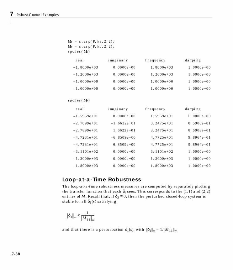
7 Robust Control Examples
7-3
Ma = starp(P,ka,2,2);Mb = starp(P,kb,2,2);spoles(Ma)
spoles(Mb)
Loop-at-a-Time RobustnessThe loop-at-a-time robustness measures are computed by separately plottingthe transfer function that each δi sees. This corresponds to the (1,1) and (2,2)entries of M. Recall that, if δ2 ≡ 0, then the perturbed closed-loop system isstable for all δ1(s) satisfying
and that there is a perturbation δ1(s), with ||δ1||∞ = 1/||M11||∞
real imaginary frequency damping
–1.8000e+03 0.0000e+00 1.8000e+03 1.0000e+00
–1.2000e+03 0.0000e+00 1.2000e+03 1.0000e+00
–1.0000e+00 0.0000e+00 1.0000e+00 1.0000e+00
–1.0000e+00 0.0000e+00 1.0000e+00 1.0000e+00
real imaginary frequency damping
–1.5959e+01 0.0000e+00 1.5959e+01 l.0000e+00
–2.7899e+01 –1.6622e+01 3.2475e+01 8.5908e–01
–2.7899e+01 1.6622e+01 3.2475e+01 8.5908e–01
–4.7231e+01 –6.8509e+00 4.7725e+01 9.8964e–01
–4.7231e+01 6.8509e+00 4.7725e+01 9.8964e–01
–3.1101e+02 0.0000e+00 3.1101e+02 1.0000e+00
–1.2000e+03 0.0000e+00 1.2000e+03 1.0000e+00
–1.8000e+03 0.0000e+00 1.8000e+03 1.0000e+00
δ1 ∞1
M11 ∞-------------------<
8

MIMO Margins Using µ
that causes instability. This is the robustness test for perturbations in channel1, with no uncertainty in channel 2. Similar comments apply for the robustnesstest for perturbations in channel 2, with no uncertainty in channel 1.
The results for Ma_g (solid) and Mb_g (dashed) are computed below, and shownin Figure 7-30.
Ma_g = frsp(Ma,omega);Mb_g = frsp(Mb,omega);vplot('liv,m',sel(Ma_g,1,1),'-',sel(Mb_g,1,1),'--');vplot('liv,m',sel(Ma_g,2,2),'-',sel(Mb_g,2,2),'--');
With respect to these uncertainty weights, the closed-loop system associatedwith controller Ka (solid) has better loop-at-a-time margins than the closed-loopsystem associated with controller Kb (dashed) since the peak is lower. Note thatthis holds for both channels.
The robustness measure for simultaneous perturbations in channels 1 and 2requires the structured singular value, µ. Recall from Chapter 4 that thestructured singular value of the matrix that the perturbation sees gives anonconservative bound on the allowable simultaneous perturbations.
In this example there are two, scalar, unmodelled dynamics perturbations (i.e.,complex blocks), so the uncertainty structure is
The µ-Tools representation of the uncertainty set, along with the µ calculationsyntax are given as follows.
∆ :=δ1 0
0 δ2
: δ1 C δ2 C∈,∈
7-39

7 Robust Control Examples
7-4
Figure 7-30 Loop-at-a-Time Robustness Tests
deltaset = [1 1;1 1];[bnds_a,dvec_a,sens_a,pvec_a] = mu(Ma_g,deltaset);[bnds_b,dvec_b,sens_b,pvec_b] = mu(Mb_g,deltaset);vplot('liv,m',bnds_a,'-',bnds_b,'--');
Plots of µ∆(M(jω)) for both closed-loop systems are shown in Figure 7-31. Notethat bnds_a and bnds_b each contain upper and lower bounds for µ, hence thereare a total of four plots in Figure 7-31. In the case of two complex uncertainties,the upper and lower bound for µ are guaranteed to be equal, so it appears thatthere are only 2 plots in the figure.
The peak associated with controller ka is much larger than the peak associatedwith controller kb. Again, the size of the smallest block-diagonal perturbationwhich causes instability is equal to
Hence, although the margins to loop-at-a-time perturbations are better withcontroller ka, the margins with respect to simultaneous perturbations aresignificantly better using controller kb.
101
100
101
102
103
104
0
0.05
0.1
0.15
0.2
0.25
0.3
0.35
0.4
0.45Channel 1 robustness: ka (solid), kb (dashed)
Frequency (rad/sec)
Mag
nitu
de
101
100
101
102
103
104
0
0.05
0.1
0.15
0.2
0.25
0.3
0.35Channel 2 robustness: ka (solid), kb (dashed)
Frequency (rad/sec)
Mag
nitu
de
1maxωµ∆ M jω( )( )--------------------------------------------
0

MIMO Margins Using µ
Figure 7-31 Structured Singular Value Plot
Constructing Destabilizing PerturbationsConstructing the smallest destabilizing perturbation for a closed-loop systemis quite useful. This perturbation can provide physical insight to the types ofvariations for which the closed-loop system is very sensitive. The commanddypert is used to construct the smallest destabilizing perturbation from theoutput of mu. The program dypert is a block-structured version of sisorat. Thedata required from the mu calculation is the perturbation vector, pvec, the blockstructure, deltaset, and the bounds for µ, bnds. Based on this data, dypertcreates a real-rational, block structured perturbation that causes instability.The ||⋅ ||∞ norm of the block diagonal perturbation is equal to 1/(peak value µ)from the associated µ plot. From the µ plot in Figure 7-31, the peak lower boundµ value for Ma_g is about 1.47 and for Mb_g, 0.64. Therefore, the H∞ norm of thesmallest destabilizing perturbation for Ma_g is , while for Mb_g we get
. The following commands illustrate this fact.
101
100
101
102
103
104
0
0.5
1
1.5Structured singular value with: ka(solid), kb (dashed)
Frequency (rad/sec)
mu
11.47----------- 0.68≈
10.64----------- 1.55≈
7-41

7 Robust Control Examples
7-4
perta = dypert(pvec_a,deltaset,bnds_a);pertb = dypert(pvec_b,deltaset,bnds_b);[pkvnorm(sel(bnds_a,1,2)) 1/pkvnorm(sel(bnds_a,1,2))]ans =
1.4657 0.6823[pkvnorm(sel(bnds_b,1,2)) 1/pkvnorm(sel(bnds_b,1,2))]ans =
0.6435 1.5540hinfnorm(perta)norm between 0.6823 and 0.6829achieved near 0hinfnorm(pertb)norm between 1.554 and 1.556achieved near 2.182
The destabilizing perturbations, perta and pertb, have the same structure as∆, block-diagonal. Therefore, the diagonal entries of perta and pertb will havenorms of 0.68 and 1.55, respectively, with zero off diagonal entries. Thefollowing commands verify this fact. The output of these functions is notshown.
hinfnorm(sel(perta,1,1))hinfnorm(sel(perta,1,2))hinfnorm(sel(perta,2,1))hinfnorm(sel(perta,2,2))hinfnorm(pertb)hinfnorm(sel(pertb,1,1))hinfnorm(sel(pertb,1,2))hinfnorm(sel(pertb,2,1))hinfnorm(sel(pertb,2,2))
2

MIMO Margins Using µ
The perturbed closed-loop can be formed with starp. Each perturbation resultsin a pair of imaginary axis eigenvalues at the frequency associated with thepeak (across frequency) of µ∆(M(jω)).
pertclpa = starp(perta,Ma,2,2);pertclpb = starp(pertb,Mb,2,2);rifd(eig(pertclpa))
rifd(eig(pertclpb))
real imaginary frequency damping
–1.0201e–04 0.0000e+00 1.0201e–04 l.0000e+00
1.0394e–14 –l.0000e–01 l.0000e–01 –1.0394e–13
1.0394e–14 l.0000e–01 l.0000e–01 –1.0394e–13
–1.4313e+00 0.0000e+00 1.4313e+00 l.0000e+00
–1.0808e+03 0.0000e+00 1.0808e+03 l.0000e+00
–1.9334e+03 0.0000e+00 1.9334e+03 l.0000e+00
real imaginary frequency damping
-1.0550e+00 0.0000e+00 1.0550e+00 l.0000e+00
-8.0315e+00 -1.1012e+01 1.3630e+01 5.8927e-01
-8.0315e+00 1.1012e+01 1.3630e+01 5.8927e-01
2.2808e-12 -3.5565e+01 3.5565e+01 -6.4132e-14
2.2808e-12 3.5565e+01 3.5565e+01 -6.4132e-14
-9.6571e+01 0.0000e+00 9.6571e+01 l.0000e+00
-3.3746e+02 -9.4865e+01 3.5054e+02 9.6268e-01
-3.3746e+02 9.4865e+01 3.5054e+02 9.6268e-01
-1.2000e+03 0.0000e+00 1.2000e+03 l.0000e+00
-1.8000e+03 0.0000e+00 1.8000e+03 l.0000e+00
7-43

7 Robust Control Examples
7-4
Space Shuttle Robustness AnalysisThis section outlines a robust stability and robust performance analysis of theSpace Shuttle lateral axis flight control system during re-entry. It serves as ageneral illustration of the usefulness of the real and complex µ analysismethods.
The system is a simplified model of the Space Shuttle, in the final stages oflanding, as it transitions from supersonic to subsonic speeds. The material inthis chapter is based on the paper:
Doyle, J., K. Lenz, and A. Packard, “Design Examples Using µ Synthesis: SpaceShuttle Lateral Axis FCS During Re-entry,” NATO ASI Series, Modelling,Robustness, and Sensitivity Reduction in Control Systems, vol. 34,Springer-Verlag, 1987.
The analysis procedure involves several steps:
1 Build uncertain model of plant.
2 Define performance specifications and uncertainty bounds.
3 Construct open-loop interconnection.
4 Close feedback loop with controller.
5 Perform a variety of real and complex µ analysis tests on the closed-loopsystem, and explore the impact of the uncertainty model (real vs. complex)on the robust stability and robust performance requirements.
6 Construct worst-case perturbations, and see their effect on the closed-loopsystem in the frequency and time domain.
4

Space Shuttle Robustness Analysis
Aircraft Model: Rigid-BodyThe rigid body model for the aircraft at Mach 0.9 is a four-state system, withstates
An input/output block diagram of the aircraft is shown in Figure 7-32.
Figure 7-32 Input-Output Description of the Aircraft
The three inputs to the aircraft are denoted by u,
The first input is the actual angular deflection of the elevon surface. The secondis the actual deflection of the rudder surface. Finally, there is a lateral windgust disturbance input, due to the winds that occur at this altitude.
There are four output variables of the aircraft. Three of these are states, whilethe fourth is the lateral acceleration at the pilot's location, denoted ny (units ofny are ft/sec2).
x
βprφ
sideslip angle (rad)roll rate (rad/s)yaw rate (rad/s)bank angle (rad)
= =
AC
ele
rud
dgust
p
r
ny
u
θele(rad)
θrud(rad)
dgust(ft/sec)
=
y
pr
ny
φ
=
7-45

7 Robust Control Examples
7-4
All variables in y are measured with inertial devices (gyroscopes andaccelerometers) whose individual noise characteristics are discussed later.
Aircraft Model: Aerodynamic UncertaintyThe major source of uncertainty in the aircraft model (AC) is in the aerodynamiccoefficients. These are standard aerodynamic parameters which expressincremental forces and torques generated by incremental changes in sideslip,elevon, and rudder angles. This is a linear relationship, expressed as
The coefficients c•• are typically estimated based on theoretical predictions,numerical calculations, experiments in wind tunnels, and flight tests. At Mach0.9, the shuttle is in a transonic regime involving a combination of subsonic andsupersonic flows. Theoretical, computational, and wind tunnel techniques areinaccurate at this flight condition, so with extremely limited flight data (earlyin the shuttle program), the coefficient uncertainty for the shuttle model isunusually large.
Uncertainty in these coefficients is modeled as a nominal value, plus aperturbation.
where the values of the r•• are
side forceyawing momentrolling moment
cyβ cya cyr
cηβ cηa cηr
clβ cla clr
βθele
θrud
=
cyβ cya cyr
cηβ cηa cηr
clβ cla clr
cyβ cya cyr
cηβ cηa cηr
clβ cla clr
ryβδyβ ryaδya ryrδyr
rηβδηβ rηaδηa rηrδηr
rlβδlβ rlaδla rlrδlr
+=
6

Space Shuttle Robustness Analysis
and the perturbations δ•• are assumed to be fixed, unknown, real parameters,with each satisfying |δ••| ≤ 1. We use the notation r••. * δ•• to denote the 3 ×3 perturbation matrix in the model for the aero coefficients, c••.
The aircraft model acnom has the nominal aerodynamic coefficients absorbedinto the state-space data. In addition to the inputs µ and outputs y describedearlier, acnom has three fictitious inputs and outputs such that the uncertainbehavior of the aircraft AC is given by the linear fractional transformation inFigure 7-33.
The state-space model for acnom is created by the M-file mk_acnom. A listing ofstate-space model acnom is given in “Shuttle Rigid Body Model” at the end ofthis section.
Figure 7-33 Uncertain Aircraft Model
ryβ rya ryr
rηβ rηa rηr
rlβ rla rlr
2.19 1.33– 0.37–
1.52– 1.35 0.870.72– 0.52 0.24
=
7-47

7 Robust Control Examples
7-4
Actuator ModelsThe aircraft has two controlled inputs, rudder command, and elevon command.Each actuator is modeled with a second order transfer function, as well as asecond order delay approximation to model the effects of the digitalimplementation.
The model for the rudder is
Here, urud is the electrical command that the controller will generate to movethe rudder. The transfer function Wdelay is a second order approximation of adelay, to model the effects of the digital implementation of the control system.In particular
with ωdel = 173 rad/s, and ξdel = 0.866. The transfer function
models the physical devices (motors, inertias, etc.) involved in actually movingthe rudder. The variable θrud is the actual deflection of the rudder surface,while urud represents the command to the rudder system. The values of theparameters are ξrud = 0.75, ωrud =21 rads/sec.
A similar model is used for the elevon actuation system. The parameters inthat case are ξele = 0.72, ωele =14 rads/sec, with an identical second order delaymodel.
The state-space models for the actuators are created by the M-file mk_act.Since the closed-loop performance objectives include penalties on the
!2ruds2+2rud!ruds+!
2rud
Wdelay
urudvrudrud
Wdelay s( )1 2ξdel– s ωdel⁄( ) s2 ωdel
2⁄( )+
1 2ξdel+ s ωdel⁄( ) s2 ωdel2⁄( )+
------------------------------------------------------------------------------=
ωrud2
s2 2ξrudωruds ωrud2
+ +------------------------------------------------------------
8
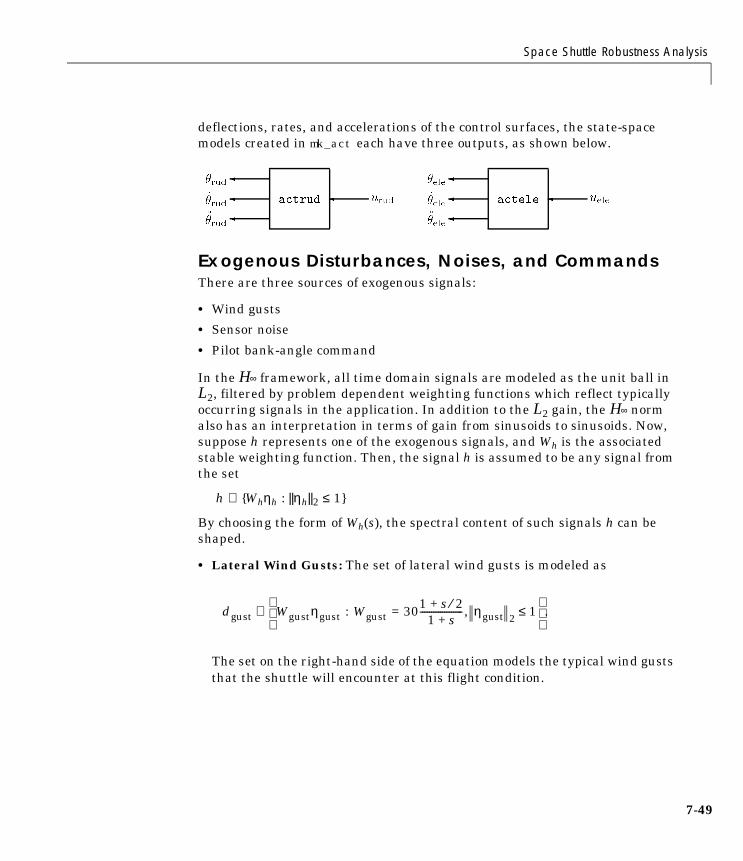
Space Shuttle Robustness Analysis
deflections, rates, and accelerations of the control surfaces, the state-spacemodels created in mk_act each have three outputs, as shown below.
Exogenous Disturbances, Noises, and CommandsThere are three sources of exogenous signals:
• Wind gusts
• Sensor noise
• Pilot bank-angle command
In the H∞ framework, all time domain signals are modeled as the unit ball inL2, filtered by problem dependent weighting functions which reflect typicallyoccurring signals in the application. In addition to the L2 gain, the H∞ normalso has an interpretation in terms of gain from sinusoids to sinusoids. Now,suppose h represents one of the exogenous signals, and Wh is the associatedstable weighting function. Then, the signal h is assumed to be any signal fromthe set
h ∈ Whηh : ||ηh||2 ≤ 1
By choosing the form of Wh(s), the spectral content of such signals h can beshaped.
• Lateral Wind Gusts: The set of lateral wind gusts is modeled as
The set on the right-hand side of the equation models the typical wind guststhat the shuttle will encounter at this flight condition.
actrud
urud
rud
_rud
rud
actele
uele
ele
_ele
ele
dgust Wgustηgust : Wgust 30=1 s 2⁄+
1 s+------------------- , ηgust 2 1≤
.∈
7-49

7 Robust Control Examples
7-5
• Sensor Noise: Each measurement is corrupted with sensor noise whichbecomes more severe with increasing frequency. Since p and r are measuredwith comparable gyroscopes, their sensor noise weights are identical,
These weighting functions imply a low frequency measurement error in pand r of 0.0003 rads/sec, and a high frequency error of 0.015 rads/sec. Themodel of the measured value of p, denoted pmeas, is given by
pmeas = p + Wpηp
where ηp is an arbitrary signal, with ||ηp||2 ≤ 1. This type of weighted, additiveL2 sensor noise is assumed for each of the 4 measured variables.
The measurement of φ is obtained from a navigation package at a reducedsample rate, so its weight is chosen to be
which is relatively large in the mid-to-high frequency range. The sensornoise weight on the ny accelerometer is
For the variables r, φ, and ny, we have
• Pilot Bank-Angle Command: In this problem, the pilot (or autopilot) takesthe shuttle through a series of sweeping “S” turns to slow the vehicle down.
WP Wr 0.00031 s/0.01+1 s/0.5+
--------------------------= =
Wφ 0.00071 s/0.01+1 s/2+
--------------------------=
Wny0.25
1 s/0.05+1 s/10+
--------------------------=
rmeas r Wrηr+=
φmeas φ Wφηφ+=
nymeasny Wny
ηny+=
0

Space Shuttle Robustness Analysis
These require accurate tracking of a bank-angle command. Typicalbank-angle commands are modeled as
φcmd = Wφcmdηφcmd,
where ηφcmd is assumed to be an arbitrary signal with ||ηφcmd||2 ≤ 1. In thisexample, the weight on the bank-angle command is chosen as
The particular choice roughly implies that the bank-angle commands aredominated by low frequency signals, with a maximum magnitude ofapproximately 0.5 radians.
The noise weighting functions are denoted by Wnoise = diagWp, Wr, Wφ, in the control block diagram.
ErrorsThere are several variables that are to be kept small in the face of theexogenous signals listed in the previous section. In this context, these variableswill be considered errors.
Actuator signal levels: the angular position, angular rates, and angularaccelerations of the rudder (⋅ rud) and elevon (⋅ ele) surfaces should remainreasonably small in the face of the exogenous signals. The signals are weightedto give an actuator error vector of
Wφcmd := 0.5 1 s/2+1 s/0.5+----------------------
Wny
eact
ee
ee·
ee
er
er·
er
:=
4 θele
θ·ele
0.005 θele
2 θrud
0.2 θ·rud
0.009 θrud
=..
..
..
..
7-51

7 Robust Control Examples
7-5
This performance specification can be loosely interpreted as a requirementthat the closed-loop system should, under the excitation of the modeledexogenous signals, maintain θele to below 0.25 radians, to below 1 rad/sec, to below 200 rads/sec2, and so on for the rudder variables. Fornotational purposes, let Wact be the 6 × 6 constant matrix so that
• Performance variables:
- The ideal bank angle response (φideal) of the shuttle to a bank-anglecommand (φcmd) is
where ω = 1.2 rad/sec, and ξ = 0.7. The bank-angle tracking error is definedas φ – φideal.
- Turn coordination: in an ideal turn, the bank angle, and the yaw rate arerelated. For this aircraft, a turn coordination error is defined as
rp := r – 0.037φ
- In a turn, it is desired that the pilot feel very little lateral acceleration,hence, the lateral acceleration variable, ny, is an error.
These error signals are weighted by frequency dependent weights to givea performance error vector as
θ·eleθele..
eact Wact
θele
θ·ele
θele
θrud
θ·rud
θrud
=
..
..
φideal :=1
1 2 ξ(s/ω ) (s/ω )2+⋅+
---------------------------------------------------------φcmd
2
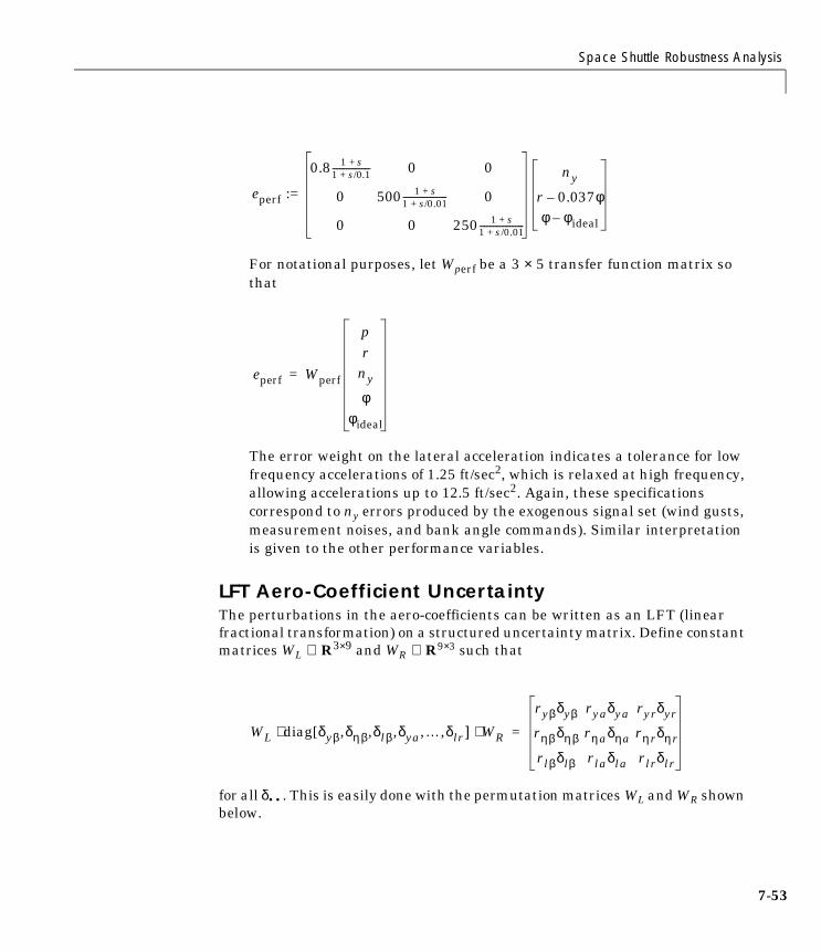
Space Shuttle Robustness Analysis
For notational purposes, let Wperf be a 3 × 5 transfer function matrix sothat
The error weight on the lateral acceleration indicates a tolerance for lowfrequency accelerations of 1.25 ft/sec2, which is relaxed at high frequency,allowing accelerations up to 12.5 ft/sec2. Again, these specificationscorrespond to ny errors produced by the exogenous signal set (wind gusts,measurement noises, and bank angle commands). Similar interpretationis given to the other performance variables.
LFT Aero-Coefficient UncertaintyThe perturbations in the aero-coefficients can be written as an LFT (linearfractional transformation) on a structured uncertainty matrix. Define constantmatrices WL ∈ R3×9 and WR ∈ R9×3 such that
for all δ••. This is easily done with the permutation matrices WL and WR shownbelow.
eperf :=
0.8 1 s+1 s/0.1+---------------------- 0 0
0 500 1 s+1 s/0.01+-------------------------- 0
0 0 250 1 s+1 s /0.01+--------------------------
ny
r 0.037φ–
φ φideal–
eperf Wperf
pr
ny
φφideal
=
WL diag[δyβ,δηβ,δlβ,δya,…,δlr ] WR⋅ ⋅
ryβδyβ ryaδya ryrδyr
rηβδηβ rηaδηa rηrδηr
rlβδlβ rlaδla rlrδlr
=
7-53

7 Robust Control Examples
7-5
Create Open-Loop InterconnectionThe aircraft model, actuator models, and weighting functions discussed in theprevious sections can be constructed from M-files.
mk_acnom;mk_act;mk_wts;
The open-loop interconnection structure, which includes the uncertainty modeland the performance objectives, is shown in Figure 7-34.
WRT
1 1 1 0 0 0 0 0 00 0 0 1 1 1 0 0 00 0 0 0 0 0 1 1 1
=
WL
2.19 0 0 1.33– 0 0 0.37– 0 00 1.52– 0 0 1.35 0 0 0.87 00 0 0.72– 0 0 0.52 0 0 0.24
=
4
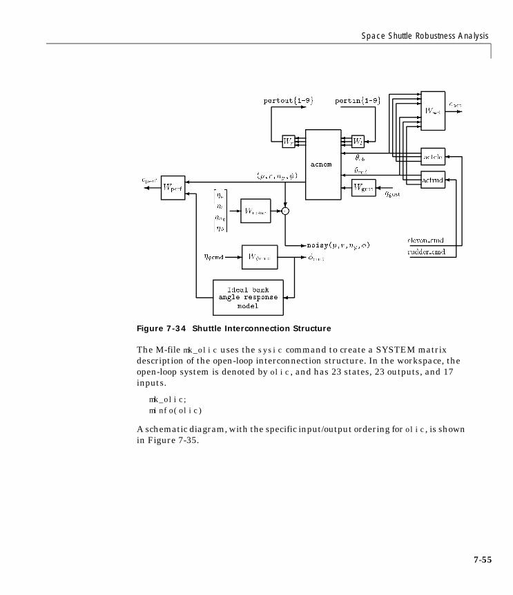
Space Shuttle Robustness Analysis
Figure 7-34 Shuttle Interconnection Structure
The M-file mk_olic uses the sysic command to create a SYSTEM matrixdescription of the open-loop interconnection structure. In the workspace, theopen-loop system is denoted by olic, and has 23 states, 23 outputs, and 17inputs.
mk_olic;minfo(olic)
A schematic diagram, with the specific input/output ordering for olic, is shownin Figure 7-35.
Ideal bankangle response
model
Wcmd-cmd - cmdcmd
noisy(p,r,ny,)rudder cmd
- elevon cmd
Wnoise-
26664
p
r
ny
37775
- h?
Wperf eperf
(p,r,ny,)
acnom
-pertoutf1-9g
Wr
Wl
pertinf1-9g
gust
Wgust
actrud
rud
acteleele
Wact
---
---
-eact
7-55

7 Robust Control Examples
7-5
Figure 7-35 Schematic Diagram of Space Shuttle olic
olic
pertinf1gpertinf2gpertinf3gpertinf4gpertinf5gpertinf6gpertinf7gpertinf8gpertinf9g
exogenous
disturbances
prnygustcmd
uelevon cmd
rudder cmd
1
2
3
4
5
6
7
8
9
10
11
12
13
14
15
16
17
pertoutf1gpertoutf2gpertoutf3gpertoutf4gpertoutf5gpertoutf6gpertoutf7gpertoutf8gpertoutf9g
eperf
weighted nyweighted r
weighted err
eact
weighted elevon acc
weighted elevon rate
weighted elevon pos
weighted rudder acc
weighted rudder rate
weighted rudder pos
y
cmd
noisy p
noisy r
noisy nynoisy
1
2
3
4
5
6
7
8
9
10
11
12
13
14
15
16
17
18
19
20
21
22
23
6

Space Shuttle Robustness Analysis
ControllersIn this section, the robustness properties of three different controllers areanalyzed using µ. The controllers receive four sensor measurements along withthe φ command signal and produce two control signals for the elevon andrudder commands. The controller block diagram is shown below.
In this example, each controller has different characteristics:
• k_h is designed to optimize H∞ performance, under the assumption thatthere is no model uncertainty;
• k_mu is designed with the D – K iteration approach to µ -synthesis;
• k_x is constructed to be a tradeoff between the two controllers
The µ-Tools commands to design the H∞ optimal controller, k_h, are:
olic_h = sel(olic,[10:23],[10:17]);minfo(olic_h)k_h = hinfsyn(olic_h,5,2,0,5,0.1);
The first command, sel, removes the aero-coefficient uncertainty channels,leaving only the exogenous signals and errors, and feedback signals. The thirdcommand, hinfsyn, designs a suboptimal H∞ controller for the open-loopsystem olic_h. This controller measures five signals, and generates twocontrol signals.
It is simple to check some characteristics of the controller and the closed-loopsystem
minfo(k_h)clp_h = starp(olic,k_h,5,2);rifd(spoles(clp_h))rifd(spoles(k_h))
K
cmd
noisy p
noisy r
noisy nynoisy
rudder cmd
elevon cmd
7-57

7 Robust Control Examples
7-5
The two other controllers have already been designed and stored in the fileshutcont.mat.
load shutcontminfo(k_x)minfo(k_mu)
Nominal Frequency ResponsesThe closed-loop system is constructed using the star product command starp.
In the closed-loop system, there are six exogenous signals (the six η signals:four sensor noises, wind gust, bank angle command) and nine errors (weightedperformance error vector and the weighted actuator error vector). The nominalperformance objective is that this multivariable transfer function matrixshould have an H∞ norm less than 1. Using µ-Tools, it is easy to evaluate thisperformance criterion. Simply form the closed-loop system, calculate itsfrequency response, and plot the norm of the appropriate transfer functionversus frequency.
8
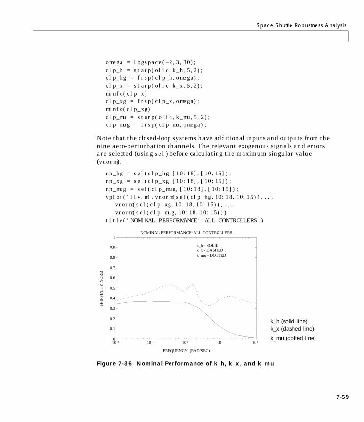
Space Shuttle Robustness Analysis
omega = logspace(–2,3,30);clp_h = starp(olic,k_h,5,2);clp_hg = frsp(clp_h,omega);clp_x = starp(olic,k_x,5,2);minfo(clp_x)clp_xg = frsp(clp_x,omega);minfo(clp_xg) clp_mu = starp(olic,k_mu,5,2);clp_mug = frsp(clp_mu,omega);
Note that the closed-loop systems have additional inputs and outputs from thenine aero-perturbation channels. The relevant exogenous signals and errorsare selected (using sel) before calculating the maximum singular value(vnorm).
np_hg = sel(clp_hg,[10:18],[10:15]);np_xg = sel(clp_xg,[10:18],[10:15]);np_mug = sel(clp_mug,[10:18],[10:15]);vplot('liv,m',vnorm(sel(clp_hg,10:18,10:15)),...
vnorm(sel(clp_xg,10:18,10:15)),...vnorm(sel(clp_mug,10:18,10:15)))
title('NOMINAL PERFORMANCE: ALL CONTROLLERS')
Figure 7-36 Nominal Performance of k_h, k_x, and k_mu
0
0.1
0.2
0.3
0.4
0.5
0.6
0.7
0.8
0.9
1
10-2 10-1 100 101 102
NOMINAL PERFORMANCE: ALL CONTROLLERS
FREQUENCY (RAD/SEC)
H-I
NF
INIT
Y N
OR
M
k_h - SOLIDk_x - DASHEDk_mu - DOTTED
k_h (solid line)k_x (dashed line)k_mu (dotted line)
7-59

7 Robust Control Examples
7-6
Note that the best nominal performance is achieved by controller k_h, as seenin Figure 7-36. This is not surprising, since it was designed specifically withthese disturbances and errors in mind. Relatively, the performance from k_muis poor, though it does meet the nominal performance objective. In latercalculations, it will become clear that the degradation in nominal performanceis offset by a much greater insensitivity to variations in the aerodynamiccoefficients.
Robust StabilityUsing µ, the robust stability characteristics of each closed-loop system can beevaluated. The uncertain parameters (δyβ,. . .,δlr) can be assumed to be real,representing uncertainty in the constant aerodynamic coefficients. However,the flow around the vehicle is very complex, and the quasi-steady implicationof constant aerodynamic coefficients is somewhat simplistic. Consequently, fora more conservative analysis, the uncertain parameters can be treated ascomplex. In this section, both models of uncertainty will be analyzed, andcompared. Refer to Chapter 4, “Modeling and Analysis of Uncertain Systems”for more detail on the interpretations.
This motivates two separate representations of the uncertainty set,
where the perturbations represent uncertainty in the aero-coefficients. Notethat the first set contains all complex perturbations, while the second setincludes only real perturbations.
In the µ-Tools syntax, these are represented as
delsetrs_C = ones(9,2);delsetrs_R = [-ones(9,1) zeros(9,1)];
Here, the lower case rs refers to robust stability (as opposed to robustperformance, rp, which will be addressed later).
The perturbation inputs/outputs from the frequency responses are selected fora robust stability µ test. The input/output channels associated with theperformance criterion are not used in the robust stability µ test. A diagram ofthe closed-loop system is shown in Figure 7-37.
∆C := diag δ1,δ2,…,δ9[ ] : δi C∈
∆R := diag δ1,δ2,… ,δ9[ ] : δi R∈
0
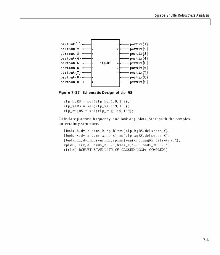
Space Shuttle Robustness Analysis
Figure 7-37 Schematic Design of clp_RS
clp_hgRS = sel(clp_hg,1:9,1:9);clp_xgRS = sel(clp_xg,1:9,1:9);clp_mugRS = sel(clp_mug,1:9,1:9);
Calculate µ across frequency, and look at µ plots. Start with the complexuncertainty structure.
[bnds_h,dv_h,sens_h,rp_h]=mu(clp_hgRS,delsetrs_C);[bnds_x,dv_x,sens_x,rp_x]=mu(clp_xgRS,delsetrs_C);[bnds_mu,dv_mu,sens_mu,rp_mu]=mu(clp_mugRS,delsetrs_C);vplot('liv,d',bnds_h,'-',bnds_x,'--',bnds_mu,'-.')title('ROBUST STABILITY OF CLOSED-LOOP: COMPLEX')
clp RS
pertinf1gpertinf2gpertinf3gpertinf4gpertinf5gpertinf6gpertinf7gpertinf8gpertinf9g
1
2
3
4
5
6
7
8
9
pertoutf1gpertoutf2gpertoutf3gpertoutf4gpertoutf5gpertoutf6gpertoutf7gpertoutf8gpertoutf9g
1
2
3
4
5
6
7
8
9
7-61
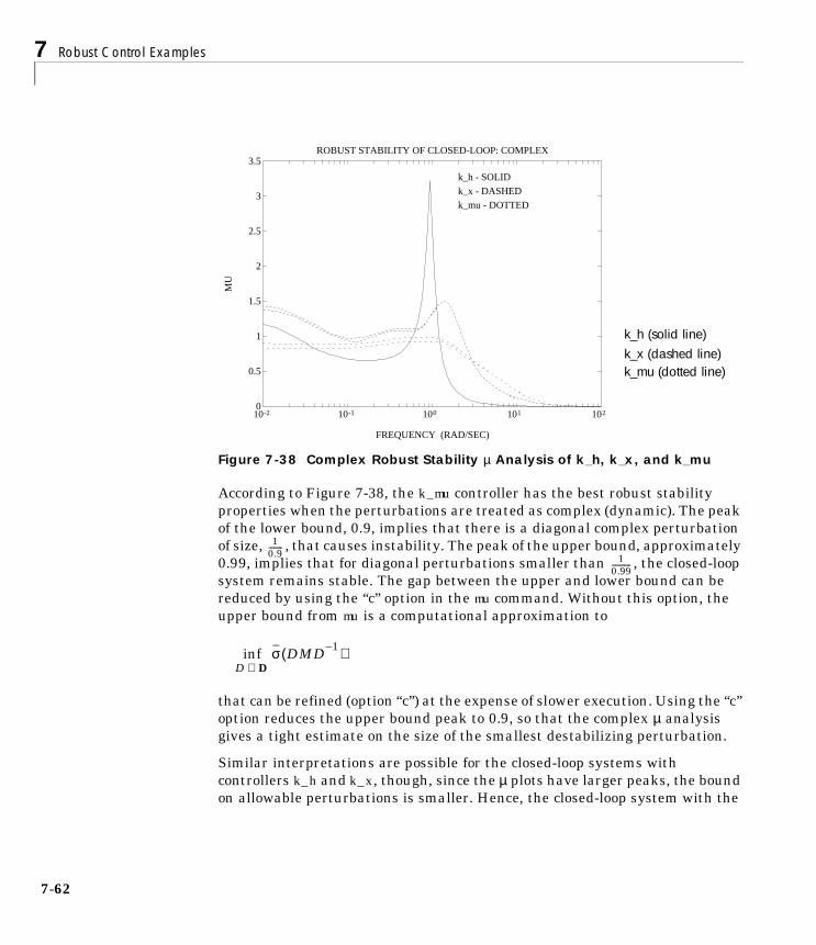
7 Robust Control Examples
7-6
Figure 7-38 Complex Robust Stability µ Analysis of k_h, k_x, and k_mu
According to Figure 7-38, the k_mu controller has the best robust stabilityproperties when the perturbations are treated as complex (dynamic). The peakof the lower bound, 0.9, implies that there is a diagonal complex perturbationof size, , that causes instability. The peak of the upper bound, approximately0.99, implies that for diagonal perturbations smaller than , the closed-loopsystem remains stable. The gap between the upper and lower bound can bereduced by using the “c” option in the mu command. Without this option, theupper bound from mu is a computational approximation to
that can be refined (option “c”) at the expense of slower execution. Using the “c”option reduces the upper bound peak to 0.9, so that the complex µ analysisgives a tight estimate on the size of the smallest destabilizing perturbation.
Similar interpretations are possible for the closed-loop systems withcontrollers k_h and k_x, though, since the µ plots have larger peaks, the boundon allowable perturbations is smaller. Hence, the closed-loop system with the
0
0.5
1
1.5
2
2.5
3
3.5
10-2 10-1 100 101 102
ROBUST STABILITY OF CLOSED-LOOP: COMPLEX
FREQUENCY (RAD/SEC)
MU
k_h - SOLID
k_x - DASHED
k_mu - DOTTED
k_h (solid line)k_x (dashed line)k_mu (dotted line)
10.9--------
10.99-----------
inf σ DMD 1–( )D D∈
2

Space Shuttle Robustness Analysis
controller k_mu achieves robust stability to complex perturbations, whereas theother controllers do not.
The closed-loop system is also analyzed treating the aerodynamic uncertaintyas real perturbations with the µ-Tools mu command.
[rbnds_h,rrp_h] = mu(clp_hgRS,delsetrs_R);[rbnds_x,rrp_x] = mu(clp_xgRS,delsetrs_R);[rbnds_mu,rrp_mu] = mu(clp_mugRS,delsetrs_R);vplot('liv,d',rbnds_h,'-',rbnds_x,'--',rbnds_mu,'-.')title('ROBUST STABILITY OF CLOSED-LOOP: REAL')
Figure 7-39 Real Robust Stability µ Analysis of k_h, k_x, and k_mu
The k_h controller has the best robust stability properties, when theperturbations are treated as real, as seen in Figure 7-39. This is in contrast tothe robust stability analysis with complex perturbation where k_mu exhibitedthe best properties. The peak of the upper bound, approximately 0.66, impliesthat for diagonal, real perturbations smaller than , the closed-loop systemremains stable. The lower bound in Figure 7-39 is often 0 and does not convergefor all values of frequency, leading to a large gap between the upper and lowerbound. This gap can be reduced by adding a small amount of complexperturbation to the pure real perturbation. A detailed discussion of this
0
0.2
0.4
0.6
0.8
1
1.2
1.4
10-2 10-1 100 101 102
ROBUST STABILITY OF CLOSED-LOOP: REAL
FREQUENCY (RAD/SEC)
MU
k_h - SOLID
k_x - DASHED
k_mu - DOTTED
k_h (solid line)k_x (dashed line)k_mu (dotted line)
10.66-----------
7-63

7 Robust Control Examples
7-6
approach can be found in the “Mixed Real/Complex Structured Singular Value”section in Chapter 4.
Robust PerformanceUsing µ, the robust performance characteristics of each closed-loop system canbe evaluated. The uncertain parameters are treated as real parameters in thisanalysis. These parameters can also be treated as complex perturbations,though this is not done in this section.
The appropriate block structure for the robust performance test is
∆P := diag[δ1,δ2,. . .,δ9,∆10] : δi ∈ R, ∆10 ∈ C6×9
which is simply an augmentation of the original real robust stabilityuncertainty set, ∆R, with a complex 6 × 9 full block to include the performanceobjectives. Recall from the “Using µ to Analyze Robust Performance” section inChapter 4: H∞ performance objectives are always represented with a full,complex block. Hence,
delsetrp_R = [delsetrs_R;6 9]
The µ calculations are performed on the entire 18 × 15 closed-loop matrix,which includes the perturbation channels and the exogenous signals anderrors. The command mu is called with both real and complex blocks.
[bnds_h,ph] = mu(clp_hg,delsetrp_R);[bnds_x,px] = mu(clp_xg,delsetrp_R);[bnds_mu,p_mu] = mu(clp_mug,delsetrp_R);vplot('liv,d',bnds_h,'-',bnds_x,'--',bnds_mu,'-.')title('ROBUST PERFORMANCE OF ALL CONTROLLERS')
4

Space Shuttle Robustness Analysis
Figure 7-40 Robust Performance µ Plots of k_h, k_x, and k_mu
The axis is selected in Figure 7-40 to show a comparison of controllers k_x andk_mu. At low frequency, the closed-loop robust performance with k_himplemented gets as bad as 14. The closed-loop system using controller k_xachieves a robust performance µ value of 1.56, while controller k_mu achieves arobust performance µ value of 1.22.
Worst-case PerturbationsUsing a µ calculation, we have seen that all controllers achieve robust-stabilityto the 9 × 9 real uncertainty matrix which represents uncertainty in theaero-coefficients. However, the performance of each closed-loop systemdegrades differently under LFT real, diagonal perturbations. We use wcperf tocompute the worst-case performance degradation as well as the worst-case,norm 1, perturbation. The worst-case perturbation of norm 1 will be used in thenext section for uncertain time-domain simulations.
[deltabadh,wcp_lowh,wcp_upph] = wcperf(clp_hg,delsetrs_R,.05,4);[deltabadx,wcp_lowh,wcp_upph] = wcperf(clp_xg,delsetrs_R,.05,10);[deltabadmu,wcp_lowmu,wcp_uppmu] = wcperf(clp_mug,delsetrs_R,.05,10);vplot(wcp_lowh,wcp_upph,wcp_lowx,wcp_uppx,wcp_lowmu,wcp_uppmu)
0
0.5
1
1.5
2
2.5
3
10-2 10-1 100 101 102
ROBUST PERFORMANCE OF ALL CONTROLLERS
FREQUENCY (RAD/SEC)
MU
k_h - SOLID
k_x - DASHED
k_mu - DOTTED
k_h (solid line)k_x (dashed line)k_mu (dotted line)
7-65
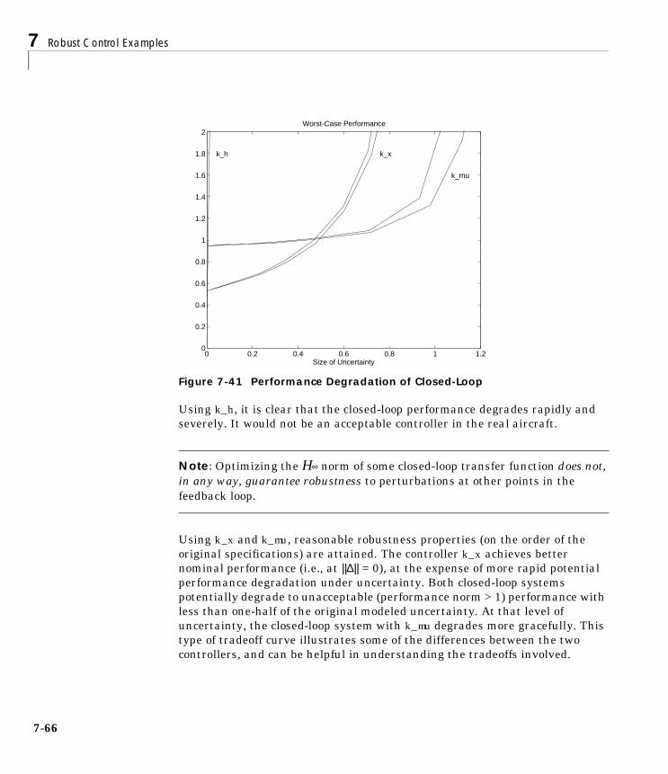
7 Robust Control Examples
7-6
Figure 7-41 Performance Degradation of Closed-Loop
Using k_h, it is clear that the closed-loop performance degrades rapidly andseverely. It would not be an acceptable controller in the real aircraft.
Note: Optimizing the H∞ norm of some closed-loop transfer function does not,in any way, guarantee robustness to perturbations at other points in thefeedback loop.
Using k_x and k_mu, reasonable robustness properties (on the order of theoriginal specifications) are attained. The controller k_x achieves betternominal performance (i.e., at ||∆|| = 0), at the expense of more rapid potentialperformance degradation under uncertainty. Both closed-loop systemspotentially degrade to unacceptable (performance norm > 1) performance withless than one-half of the original modeled uncertainty. At that level ofuncertainty, the closed-loop system with k_mu degrades more gracefully. Thistype of tradeoff curve illustrates some of the differences between the twocontrollers, and can be helpful in understanding the tradeoffs involved.
0 0.2 0.4 0.6 0.8 1 1.20
0.2
0.4
0.6
0.8
1
1.2
1.4
1.6
1.8
2
Size of Uncertainty
Worst-Case Performance
k_x
k_mu
k_h
6

Space Shuttle Robustness Analysis
Time SimulationsThe open-loop simulation interconnection, Figure 7-42, is similar to olic, butcontains none of the weighting functions. It is used exclusively for nominal andperturbed time-domain simulations, where unweighted time signals will becalculated and plotted.
mk_olsim;minfo(olsim)
Figure 7-42 Open-Loop Simulation Model
For the purposes of this exercise, the four sensor noises have been eliminatedfrom the simulation model. It is easy to modify mk_olsim.m to include these ifdesired.
The LFT time simulation GUI, simgui, is used to simulate the nominal andperturbed time response of the three controllers. For more details on simgui
olsim
pertinf1g
pertinf2gpertinf3g
pertinf4g
pertinf5g
pertinf6g
pertinf7g
pertinf8g
pertinf9gdgust
cmd
elevoncmd
ruddercmd
1
2
3
4
5
6
7
8
9
10
11
12
13
1
2
3
4
5
6
7
8
9
10
11
12
13
14
15
16
17
18
19
20
21
22
23
24
pertoutf1gpertoutf2g
pertoutf3g
pertoutf4g
pertoutf5g
pertoutf6g
pertoutf7g
pertoutf8g
pertoutf9g
ny
r c
ideal
ele_eleelerud_rudrudcmd
p
p
ny
7-67
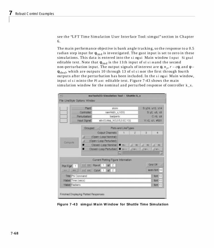
7 Robust Control Examples
7-6
see the “LFT Time Simulation User Interface Tool: simgui” section in Chapter6.
The main performance objective is bank angle tracking, so the response to a 0.5radian step input for φcmd is investigated. The gust input is set to zero in thesesimulations. This data is entered into the simgui Main window Input Signaleditable text. Note that φcmd is the 11th input of olsim and the secondnon-perturbation input. The output signals of interest are φ, ny, r – cφ, and φ –φideal, which are outputs 10 through 13 of olsim or the first through fourthoutputs after the perturbation has been included. In the simgui Main window,input olsim into the Plant editable text. Figure 7-43 shows the mainsimulation window for the nominal and perturbed response of controller k_x.
Figure 7-43 simgui Main Window for Shuttle Time Simulation
8

Space Shuttle Robustness Analysis
We are interested in the nominal and perturbed closed-loop response in thepresence of a worst-case, real perturbation. This corresponds to the top ninechannels of olsim, the aero-coefficient perturbations. Therefore, worst-casereal perturbations of size 1 in the aero-coefficients for k_x and k_mu arecalculated using the wcperf command. These perturbations are:
badpertx is used in the perturbed response for controller k_x and badpertmu isused as the worst-case real perturbation for controllers k_h and k_mu. This datais input into the Perturbation editable text in the simgui main window.
The controllers are implemented in discrete-time at a sample-rate of 20Hz onthe shuttle. To replicate the same implementation, a sample-data timesimulation is performed. This simulation is available under the Options menuin the Main simulation window. Therefore, the continuous-time controllers,k_x, k_h, and k_mu, must be discretized for the sampled-data time simulation.The continuous-time plant, olsim, is simulated at 200Hz and the controllers at20Hz as seen in the simgui parameter window, Figure 7-44.
Figure 7-44 simgui Parameter Window for Shuttle Time Simulation
badpertx = diag([ 1 1 1 –.87 1 1 –.28 –1 –1 ])
badpertmu = diag([ –1 –1 –1 1 1 1 –1 –1 –1 ])
7-69
7 Robust Control Examples
7-7
The nominal and perturbed closed-loop responses with k_x, k_h, and k_muimplemented are shown in Figure 7-45 and Figure 7-46. As expected, the timedomain simulations reinforce the conclusions that were reached in thefrequency domain analysis. The nominal performance associated with k_h issuperb, but degrades significantly with the aerodynamic uncertainty. In thatrespect, the controller k_mu performs the best, nearly achieving all of the robustperformance objectives. The nominal and perturbed time response of otherperformance variables can also be easily investigated.
0

Space Shuttle Robustness Analysis
Figure 7-45 Closed-Loop Nominal and Perturbed Time Response, k_x (top) and k_h
nominal (solid line) perturbed (dashed line)
7-71

7 Robust Control Examples
7-7
Figure 7-46 Closed-Loop Nominal and Perturbed Time Response, k_mu
ConclusionsThis exercise illustrated the use of the µ-Tools software to analyze the robuststability and robust performance objectives on a complicated, uncertain plantmodel.
There is an important feature of the mu software that cannot be overlooked oroveremphasized. These algorithms calculate both upper and lower bounds forµ, and produce worst-case perturbations which provide the lower bound. Theperturbations, and their effects, can be analyzed in both the frequency domainand time domain. In practice, the bad perturbations are also used in highfidelity, nonlinear simulations of the closed-loop system to discover limitationsand unforeseen problems.
Nominal (solid line) Perturbed (dashed line)
2

Space Shuttle Robustness Analysis
Although this problem did not have repeated uncertain parameters (each δ••appeared only once), the algorithms and software do handle these cases, andthe reader is referred back to the “Complex Structured Singular Value” sectionin Chapter 4 for details.
Space Shuttle ReferencesDoyle, J., K. Lenz, and A. Packard, “Design Examples Using µ Synthesis: SpaceShuttle Lateral Axis FCS During Reentry,” NATO ASI Series, Modelling,Robustness, and Sensitivity Reduction in Control Systems, vol. 34,Springer-Verlag, 1987.
7-73
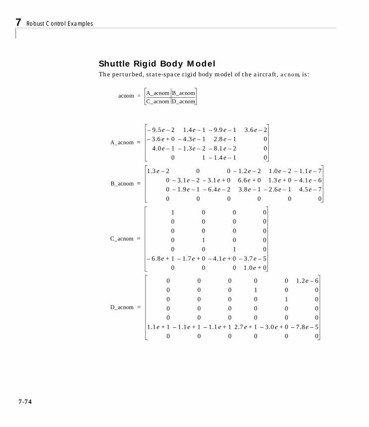
7 Robust Control Examples
7-7
Shuttle Rigid Body ModelThe perturbed, state-space rigid body model of the aircraft, acnom, is:
acnom A_acnom B_acnom
C_acnom D_acnom=
A_acnom
9.5e– 2– 1.4e 1– 9.9e– 1– 3.6e 2–
3.6e– 0+ 4.3e– 1– 2.8e 1– 04.0e 1– 1.3e– 2– 8.1e– 2– 0
0 1 1.4e– 1– 0
=
B_acnom
1.3e 2– 0 0 1.2e– 2– 1.0e 2– 1.1e– 7–
0 3.1e– 2– 3.1e– 0+ 6.6e 0+ 1.3e 0+ 4.1e– 6–
0 1.9e– 1– 6.4e– 2– 3.8e 1– 2.6e– 1– 4.5e 7–
0 0 0 0 0 0
=
C_acnom
1 0 0 00 0 0 00 0 0 00 1 0 00 0 1 0
6.8e– 1+ 1.7e– 0+ 4.1e– 0+ 3.7e– 5–
0 0 0 1.0e 0+
=
D_acnom
0 0 0 0 0 1.2e 6–
0 0 0 1 0 00 0 0 0 1 00 0 0 0 0 00 0 0 0 0 0
1.1e 1+ 1.1e– 1+ 1.1e– 1+ 2.7e 1+ 3.0e– 0+ 7.8e– 5–
0 0 0 0 0 0
=
4

HIMAT Robust Performance Design Example
HIMAT Robust Performance Design ExampleThis section contains an idealized example of µ-synthesis as applied to thedesign of a pitch axis controller of an experimental highly maneuverableairplane, HIMAT. The airplane model is taken from aerodynamic data for theHIMAT vehicle. The problem is posed as a robust performance problem, withmultiplicative plant uncertainty at the plant input and plant output weightedsensitivity function as the performance criterion. The design procedurepresented in this section involves several steps:
1 Specification of closed-loop feedback structure.
2 Specification of model uncertainty and performance objectives in terms offrequency-dependent weighting matrices.
3 Construction of open-loop interconnection for control synthesis routines.
4 Loop shape controller design for the open-loop interconnection.
5 H∞ optimal controller design for the open-loop interconnection.
6 Analysis of robust performance properties of the resulting closed-loopsystems using the structured singular value, µ (µ-analysis).
7 Use of frequency dependent similarity scalings, obtained in the µ-analysisstep, to scale the open-loop interconnection, and redesign H∞ controller(iterating on steps 5, 6, and 7 constitutes the approach to µ-synthesis called“D – K iteration,” which is described in detail in Chapter 5).
The main objective of this section is to illustrate µ-synthesis design methods(steps 1, 2, 3, 5, 6, 7). The loop shape controller (step 4) is included to illustratethat robust stability and nominal performance do not necessarily imply robustperformance.
Many of the command outputs are not displayed in the text, since it is assumedthat the reader is simultaneously working through the example on a computer.
7-75

7 Robust Control Examples
7-7
HIMAT Vehicle Model and Control ObjectivesThe HIMAT vehicle model and control objectives are taken from a paper bySafonov et al. (1981). The interested reader should consult this paper as wellas Hartman et al. (1979) and Merkel and Whitmoyer (1976) for more details.The HIMAT vehicle was a scaled, remotely piloted vehicle (RPV) version of anadvanced fighter, which was flight tested in the late 1970s. The actual HIMATvehicle is currently on display in the Smithsonian National Aerospace Museumin Washington, D.C. The design example will consider only the longitudinaldynamics of the airplane. These dynamics are assumed to be uncoupled fromthe lateral-directional dynamics. Linearized models for a collection of flightconditions can be found in [HartBG]. The state vector consists of the vehicle'sbasic rigid body variables:
xT = (δv, α, q, θ)
representing the forward velocity, angle-of-attack, pitch rate, and pitch angle,respectively. The flight path angle (γ) is defined as γ = θ – α. The state variablesused to describe motions in the vertical plane are given below:
δv — perturbations along the velocity vector
α — angle between velocity vector and aircraft's longitudinal axis
q — rate-of-change of aircraft attitude angle
θ — aircraft attitude angle
The control inputs are the elevon (δe) and the canard (δc). The variables to bemeasured are α and θ.
There are three longitudinal maneuvers to be considered:
Vertical Translation: Control the vertical velocity at a constant θ (α varies).This implies that the attitude is held constant as the velocity vector rotates.
Pitch Pointing: Control the attitude at a constant flight path angle (i.e., θ –α = constant). In this case the velocity vector does not rotate.
Direct Lift: Control the flight path angle at constant angle-of-attack (i.e.,γ = θ). This maneuver produces a normal acceleration response withoutchanging the angle-of-attack.
These control objectives are accounted for within the performancespecification.
6
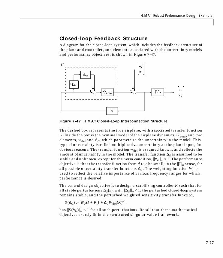
HIMAT Robust Performance Design Example
Closed-loop Feedback StructureA diagram for the closed-loop system, which includes the feedback structure ofthe plant and controller, and elements associated with the uncertainty modelsand performance objectives, is shown in Figure 7-47.
Figure 7-47 HIMAT Closed-Loop Interconnection Structure
The dashed box represents the true airplane, with associated transfer functionG. Inside the box is the nominal model of the airplane dynamics, Gnom, and twoelements, wdel and ∆G, which parametrize the uncertainty in the model. Thistype of uncertainty is called multiplicative uncertainty at the plant input, forobvious reasons. The transfer function wdel is assumed known, and reflects theamount of uncertainty in the model. The transfer function ∆G is assumed to bestable and unknown, except for the norm condition, ||∆G||∞ < 1. The performanceobjective is that the transfer function from d to e be small, in the ||⋅ ||∞ sense, forall possible uncertainty transfer functions ∆G. The weighting function WP isused to reflect the relative importance of various frequency ranges for whichperformance is desired.
The control design objective is to design a stabilizing controller K such that forall stable perturbations ∆G(s), with ||∆G||∞ < 1, the perturbed closed-loop systemremains stable, and the perturbed weighted sensitivity transfer function,
S(∆G) := WP(I + P(I + ∆GWdel)K)–1
has ||S(∆G)||∞ < 1 for all such perturbations. Recall that these mathematicalobjectives exactly fit in the structured singular value framework.
7-77
7 Robust Control Examples
7-7
Uncertainty ModelsThe airplane model we consider has two inputs: elevon command (δe) andcanard command (δc); and two measured outputs: angle-of-attack (α) and pitchangle (θ).
A first principles set of uncertainties about the aircraft model would include:
• Uncertainty in the canard and the elevon actuators. The electrical signalsthat command deflections in these surfaces must be converted to actualmechanical deflections by the electronics and hydraulics of the actuators.This is not done perfectly in the actual system, unlike the nominal model.
• Uncertainty in the forces and moments generated on the aircraft, due tospecific deflections of the canard and elevon. As a first approximation, thisarises from the uncertainties in the aerodynamic coefficients, which varywith flight conditions, as well as uncertainty in the exact geometry of theairplane. An even more detailed view is that surface deflections generate theforces and moments by changing the flow around the vehicle in very complexways. Thus there are uncertainties in the force and moment generation thatgo beyond the quasi-steady uncertainties implied by uncertain aerodynamiccoefficients.
• Uncertainty in the linear and angular accelerations produced by theaerodynamically generated forces and moments. This arises from theuncertainty in the various inertial parameters of the airplane, in addition toneglected dynamics such as fuel slosh and airframe flexibility.
• Other forms of uncertainty that are less well understood.
In this example, we choose not to model the uncertainty in this detailedmanner, but rather to lump all of these effects together into one full-blockuncertainty at the input of a four-state, nominal model of the aircraft rigidbody. This nominal model has no (i.e., perfect) actuators and only quasi-steadydynamics. The nominal model for the airplane is loaded from the mutools/subsdirectory.
8

HIMAT Robust Performance Design Example
The simple model of the airplane has four states: forward speed (v),angle-of-attack (α), pitch rate (q) and pitch angle (θ); two inputs: elevoncommand (δe) and canard command (δc); and two measured outputs:angle-of-attack (α) and pitch angle (θ).
mkhimat;minfo(himat)seesys(himat,'%9.le')
The partitioned matrix represents the [A B; C D] state space data. Given thisnominal model himat (i.e., Gnom(s)) we also specify a stable, 2 × 2 transfermatrix Wdel(s), called the uncertainty weight. These two transfer matricesparametrize an entire set of plants, G, which must be suitably controlled by therobust controller K.
G := Gnom(I + ∆GWdel) : ∆G stable, ||∆G||∞ ≤ 1.
All of the uncertainty in modeling the airplane is captured in the normalized,unknown transfer function ∆G. The unknown transfer function ∆G(s) is used toparametrize the potential differences between the nominal model Gnom(s), andthe actual behavior of the real airplane, denoted by G. The dependence onfrequency of the uncertainty weight indicates that the level of uncertainty inthe airplane's behavior depends on frequency.
In this example, the uncertainty weight Wdel is of the form Wdel(s) := wdel(s)I2,for a given scalar valued function wdel(s). The fact that the uncertainty weightis diagonal, with equal diagonal entries, indicates that the modeleduncertainty is in some sense a round ball about the nominal model Gnom. Thescalar weight associated with the multiplicative input uncertainty is
–2.3e–02 –3.7e+01 –1.9e+01 –3.2e+01 | 0.0e+00 0.0e+00
0.0e+00 –1.9e+00 9.8e–01 0.0e+00 | –4.1e–01 0.0e+00
1.2e–02 –1.2e+01 –2.6e+00 0.0e+00 | –7.8e+01 2.2e+01
0.0e+00 0.0e+00 1.0e+00 0.0e+00 | 0.0e+00 0.0e+00
------------------------------------ | -----------------
0.0e+00 5.7e+01 0.0e+00 0.0e+00 | 0.0e+00 0.0e+00
0.0e+00 0.0e+00 0.0e+00 5.7e+01 | 0.0e+00 0.0e+00
7-79

7 Robust Control Examples
7-8
constructed using the command nd2sys. The weight chosen for this problem is.
wdel = nd2sys([1 100],[1 10000],50);
The set of plants that are represented by this uncertainty weight is:
The weighting function is used to normalize the size of the unknownperturbation ∆G. At any frequency ω, |ωdel(jω)| can be interpreted as thepercentage of uncertainty in the model at that frequency.
omega = logspace(0,5,50);wdel_g = frsp(wdel,omega);vplot('liv,lm',wdel_g)title('Multiplicative Uncertainty Weighting Function')xlabel('Frequency (rad/s)')
The particular uncertainty weight chosen for this problem indicates that at lowfrequency, there is potentially a 50% modeling error, and at a frequency of 173rad/sec, the uncertainty in the model is up to 100%, and could get larger athigher and higher frequencies. A frequency response of wdel is shown in Figure7-48.
Specifications of Closed-loop PerformanceThe performance of the closed loop system will be evaluated using the outputsensitivity transfer function, (I + GK)–1. Good performance will becharacterized in terms of a weighted H∞ norm on this transfer function. Givena 2 × 2 stable, rational transfer matrix WP, we say that nominal performanceis achieved if ||WP(I + GK)–1||∞ < 1. As in the uncertainty modeling, theweighting function Wp is used to normalize specifications, in this case, to defineperformance as whether a particular norm is less than 1.
In this problem, we choose a simple weight of the form WP(s) = wp(s)I2, where
.
wdel50 s 100+( )s 10000+
-------------------------------=
G := Gnom I250 s 100+( )s 10000+
------------------------------∆G s( )+ : ∆G s( ) stable, ∆G ∞ 1≤
wp s( ) 0.5 s 3+( )s 0.03+
--------------------------=
0

HIMAT Robust Performance Design Example
Figure 7-48 HIMAT Multiplicative Uncertainty Weighting Function
wp = nd2sys([1 3],[1 0.03],0.5);
For performance to be achieved, ||WP(I + GK)–1||∞ < 1, and since WP is a scalar(times a 2 × 2 identity), the maximum singular value plot of the sensitivitytransfer function (I + GK)–1 must lie below the plot of at every frequency.That is, ||WP(I + GK)–1||∞ < 1, if and only if at all frequencies,
.
omega = logspace(–3,2,50);wp_g = frsp(wp,omega);vplot('liv,lm',minv(wp_g))title('Inverse of Performance Weighting function')xlabel('Frequency (rad/s)')
This sensitivity weight indicates that at low frequency, the closed-loop (bothnominal and perturbed) should reject disturbances at the output by a factor of50-to–1. Expressed differently, steady-state tracking errors in both channels,due to reference step-inputs in either channel should be on the order of 0.02 orsmaller. This performance requirement gets less and less stringent at higherand higher frequencies. The closed-loop system should perform better thanopen-loop for frequencies up to 1.73 radians/second, and for higher frequencies,the closed-loop performance should degrade gracefully, always lying
10-1
100
101
102
100 101 102 103 104 105
Multiplicative Uncertainty Weighting Function
Frequency (rad/s)
1wp----------
σ I GK+( ) 1– jω( )[ ] 1 wp⁄ jω( )<
7-81

7 Robust Control Examples
7-8
underneath the inverse of the weight, wp. The frequency response of isshown in Figure 7-49.
Figure 7-49 Inverse of the HIMAT Performance Weight
The 2 × 2 weighting matrices in the interconnection involve the scalar functionswe have discussed, and identity matrices of dimension 2. We can build thesematrices using the command daug, which stands for diagonal augmentation.Each new weight has two states, two inputs and two outputs as one can seeusing minfo.
wdel = daug(wdel,wdel);wp = daug(wp,wp);minfo(wdel)minfo(wp)
The engineering motivation for a performance specification like this mightcome from the desire to have independent tracking of the angle of attack andpitch angle. This allows the vehicle to be pointed in pitch independently fromvertical motions. We would expect this to be difficult to achieve, given that it isobviously easier for the vehicle to simultaneously pitch up and accelerate upthan it is to simultaneously pitch down and accelerate up.
1wp-------
10-2
10-1
100
101
10-3 10-2 10-1 100 101 102
Frequency (rad/s)
Inverse of Performance Weighting function
2
HIMAT Robust Performance Design Example
Robust Stability, Nominal Performance, Robust PerformanceThe phrases robust stability, nominal performance, and robust performanceare used in this framework extensively.
Nominal Performance. The closed-loop system achieves nominal performance ifthe performance objective is satisfied for the nominal plant model, Gnom.
In this problem, that is equivalent to:
Nominal Performance ⇔ ||WP(I + GnomK)–1||∞ < 1
Robust Stability. The closed-loop system achieves robust stability if the closedloop system is internally stable for all of the possible plant models G ∈ G.
In this problem, that is equivalent to a simple norm test on a particularnominal closed-loop transfer function.
Robust Stability ⇔ ||WdelKGnom(I + KGnom)–1||∞ < 1
Robust Performance. The closed-loop system achieves robust performance if theclosed-loop system is internally stable for all G ∈ G, and in addition to that, theperformance objective,
||WP(I + GK)–1||∞ < 1,
is satisfied for every G ∈ G. The property of robust performance is equivalentto a structured singular value test (a generalization of the two H∞ norm testsin the previous conditions) on a particular, nominal closed- loop transferfunction. This is discussed further in Chapter 4, “Modeling and Analysis ofUncertain Systems”.
Building the Open-Loop InterconnectionThe command sysic is used to construct the open-loop interconnection. We willoften refer to this open-loop system as the generalized plant. In this particularexample, we store the system in the MATLAB variable himat_ic. Thecommand sysic will build any specified interconnection of smaller subsystems,provided the correct information about the interconnection is in the MATLABworkspace.
A six-input, six-output SYSTEM matrix, himat_ic, (also referred to as P)
7-83
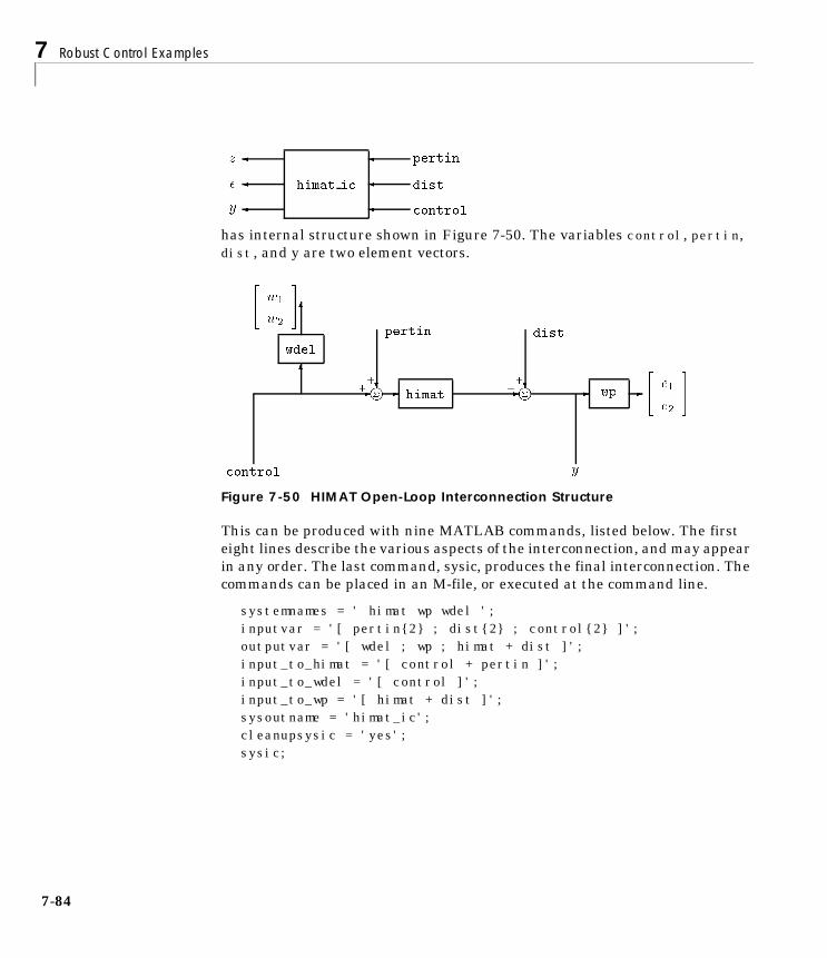
7 Robust Control Examples
7-8
has internal structure shown in Figure 7-50. The variables control, pertin,dist, and y are two element vectors.
Figure 7-50 HIMAT Open-Loop Interconnection Structure
This can be produced with nine MATLAB commands, listed below. The firsteight lines describe the various aspects of the interconnection, and may appearin any order. The last command, sysic, produces the final interconnection. Thecommands can be placed in an M-file, or executed at the command line.
systemnames = ' himat wp wdel ';inputvar = '[ pertin2 ; dist2 ; control2 ]';outputvar = '[ wdel ; wp ; himat + dist ]';input_to_himat = '[ control + pertin ]';input_to_wdel = '[ control ]';input_to_wp = '[ himat + dist ]';sysoutname = 'himat_ic';cleanupsysic = 'yes'; sysic;
pertinz
diste
controly
himat ic
4

HIMAT Robust Performance Design Example
Since the system himat_ic is still open-loop, its poles are simply the poles ofthe various components that make up the interconnection.
minfo(himat_ic)spoles(himat_ic) spoles(himat)spoles(wdel)spoles(wp)
µ-synthesis and D – K IterationFor notational purposes, let P(s) denote the transfer function of the six-input,six-output open-loop interconnection, himat_ic. Define a block structure ∆ as
The first block of this structured set corresponds to the full-block uncertainty∆G used in section to model the uncertainty in the airplane's behavior. Thesecond block, ∆2 is a fictitious uncertainty block, used to incorporate the H∞
performance objectives on the weighted output sensitivity transfer functioninto the µ-framework.
Using theorem 4.5 from the “Robust Performance” section in Chapter 4, astabilizing controller K achieves closed-loop, robust performance if and only iffor each frequency ω ∈ [0, ∞], the structured singular value
µ∆[FL(P,K)(jω)] < 1
Using the upper bound for µ, (recall that in this case, two full blocks, the upperbound is exactly equal to µ) we can attempt to minimize the peak closed-loop µvalue by posing the optimization problem
∆:=∆1 0
0 ∆2
: ∆1 C2 2×∈ ,∆2 C2 2×∈
C4 4×⊂ .
min d s( )I2 0
0 I2
FL P K,( ) d 1– s( )I2 0
0 I2 ∞K
stabilizing
mind s( )
stable,min–phase
7-85

7 Robust Control Examples
7-8
Finding the value of this minimum and constructing controllers K that achievelevels of performance arbitrarily close to the optimal level is called µ-synthesis.A more detailed discussion of D – K iteration is given in Chapter 5.
Before plunging into the D – K iteration design procedure, we begin with acontroller designed via basic MIMO loop shaping methods.
Loop Shaping Control DesignOne approach to control design for the HIMAT model is to synthesize a loopshaping controller. We want the loop shape controller, Kloop, to make theopen-loop gain act as an integrator at low frequency and at crossover. At highfrequencies, we won't worry too much about the details of the roll-off, providedthat it is at least first order. To achieve this, we'll roughly invert the plant G(s)(G has only 1 MIMO finite zero, at s ≈ −0.026; it also has zeros at s = ∞, so ourinverse is only approximate) and augment the desired loop gain dynamics tothe controller. The series of commands below constructs one such controllerand plots the open-loop gain (broken at the input to the controller), as seen inFigure 7-51. The interested reader may want to explore various alternativeschemes for constructing loop shape controllers discussed in Freudenberg andLooze (1988).
[a,b,c,d] = unpck(himat);cn = c*a*a + 1000*c*a;dn = c*a*b + 1000*c*b;kloop = mscl(minv(pck(a,b,cn,dn)),–9000);L = mmult(himat,kloop);omega = logspace(–1,4,50);Lg = frsp(L,omega);vplot('liv,lm',vsvd(Lg))title('Loop Gain Plot with Loop Shape Controller')xlabel('Frequency (rad/s)')
6

HIMAT Robust Performance Design Example
Figure 7-51 Loop Gain of the Loop Shaping Controller
The open-loop gain plot satisfies both the low frequency performance objectiveand the high frequency robustness goals. We have only plotted the singularvalues of GKloop, but KloopG looks similar. Hence, you would expect thecontroller to satisfy the robust stability and nominal performancerequirements.
The two 2 × 2 transfer functions associated with robust stability and nominalperformance can be evaluated for the loop shaping controller. Simply close theopen-loop interconnection P (himat_ic) with the loop shaping controller, Kloop(kloop) and evaluate the pertinent transfer functions using the command sel.
10-3
10-2
10-1
100
101
102
10-1 100 101 102 103 104
Loop Gain Plot with Loop Shape Controller
Frequency (rad/s)
7-87

7 Robust Control Examples
7-8
In using sel, the desired outputs (or rows) are specified first, followed by thedesired inputs (or columns). The results are seen in Figure 7-52.
clp = starp(himat_ic,kloop,2,2);spoles(clp)rs_loop = sel(clp,1:2,1:2);np_loop = sel(clp,3:4,3:4);rs_loopg = frsp(rs_loop,omega);np_loopg = frsp(np_loop,omega);vplot('liv,m',vnorm(rs_loopg),vnorm(np_loopg))tmp1 = 'ROBUST STABILITY (solid) and';tmp2 = ' NOMINAL PERFORMANCE (dashed)';title([tmp1 tmp2])xlabel('Frequency(rad/s)')
Figure 7-52 Robust Stability and Nominal Performance Plots for the Loop Shaping Controller
0.05
0.1
0.15
0.2
0.25
0.3
0.35
0.4
0.45
0.5
0.55
10-1 100 101 102 103 104
ROBUST STABILITY (solid) and NOMINAL PERFORMANCE (dashed)
Frequency (rad/s)
Robust stability (solid line) Nominal Performance (dashed line)
8

HIMAT Robust Performance Design Example
The interpretation of the plots in Figure 7-52 is as follows:
• The controlled system (with loop shaping controller) achieves nominalperformance. This conclusion follows from the singular value plot of thenominal weighted output sensitivity function, which has a peak value of0.50.
• The controlled system (with loop shaping controller) achieves robuststability. This conclusion stems from the singular value plot of the nominalweighted input complementary sensitivity function, which has a peak valueof 0.50.
H∞ Design on the Open-Loop InterconnectionIn this section, we carry out the first step of the D – K iteration, which is an H∞
(sub)optimal control, design for the open-loop interconnection, himat_ic. Interms of the iteration, this amounts to holding the d variable fixed (at 1), andminimizing the ||⋅ ||∞ norm of FL(P,K), over the controller variable K. Recall thatFL(P,K) is the nominal closed loop transfer function from the perturbationinputs and disturbances (sysic variables pertin and dist) to the perturbationoutputs and errors (z and e), shown in Figure 7-53.
Figure 7-53 Closed-Loop Linear Fractional Transformation
The function hinfsyn designs a (sub)optimal H∞ control law based on theopen-loop interconnection structure provided. Syntax, input and outputarguments of hinfsyn are:
[k,clp] = hinfsyn(p,nmeas,ncon,glow,ghigh,tol)
7-89

7 Robust Control Examples
7-90
The arguments are:
Inputs
Outputs
In this example, the open-loop interconnection is himat_ic, with twomeasurements, two control inputs, and the bisection algorithm will search forthe optimal achievable closed-loop norm, to an absolute tolerance of 0.06,between lower and upper limits of 0.8 and 6.0, respectively. Since we areplanning on performing several iterations of the D – K iteration procedure, welabel the resulting controller k1. The resulting closed loop system (4-input,4-output), from [pertin;dist] to [z;e] is labeled clp1.
[k1,clp1] = hinfsyn(himat_ic,2,2,0.8,6.0,.06);
The controller is stable, and its Bode plot is shown in Figure 7-54.
Properties of Controllerminfo(k1)omega = logspace(–1,4,50);spoles(k1)k1_g = frsp(k1,omega);vplot('bode',k1_g)subplot(211), title('Frequency Response of k1')
open-loop interconnection (SYSTEM matrix) p
number of measurements nmeas
number of controls ncons
lower bound for bisection glow
upper bound for bisection ghigh
absolute tolerance for bisection method tol
controller (SYSTEM matrix) k
closed-loop (SYSTEM matrix) clp

HIMAT Robust Performance Design Example
Figure 7-54 Bode Plot of k1
Figure 7-55 shows the singular values of the closed-loop system clp1. Althoughclp1 is 4 × 4, at each frequency it only has rank equal to 2, hence only twosingular values are nonzero.
Closed-loop Properties:rifd(spoles(clp1))clp1g = frsp(clp1,omega);clp1gs = vsvd(clp1g);vplot('liv,m',clp1gs)title('Singular Value Plot of clp1')xlabel('Frequency (rad/s)')
101
100
101
102
103
104
400
200
0
200
Pha
se (
degr
ees)
Frequency (radians/sec)
101
100
101
102
103
104
104
102
100
102
Log
Mag
nitu
de
Frequency (radians/sec)
Frequency Response of k1
7-91

7 Robust Control Examples
7-9
Figure 7-55 Singular Value Plot of the Closed-Loop System with k1
The two 2 × 2 transfer functions associated with robust stability and nominalperformance may be evaluated separately, using the command sel. Recall thatthe robust stability test is performed on the upper 2 × 2 transfer function inclp1, and the nominal performance test is on the lower 2 × 2 transfer functionin clp1. Since a frequency response of clp1 is already available, (in clp1g) wesimply perform the sel on the frequency response, and plot the norms.
rob_stab = sel(clp1g,[1 2],[1 2]);nom_perf = sel(clp1g,[3 4],[3 4]);minfo(rob_stab)minfo(nom_perf)vplot('liv,m',vnorm(rob_stab),vnorm(nom_perf))tmp1 = 'ROBUST STABILITY (solid) and';tmp2 = ' NOMINAL PERFORMANCE (dashed)';title([tmp1 tmp2])xlabel('Frequency (rad/s)')
0
0.2
0.4
0.6
0.8
1
1.2
1.4
1.6
1.8
10-1 100 101 102 103 104
Singular Value Plot of clp1
Frequency (rad/s)
2

HIMAT Robust Performance Design Example
Figure 7-56 Robust Stability and Nominal Performance Plots Using Controller k1
The interpretation of the plots in Figure 7-56 is as follows:
• The controlled system achieves nominal performance. This conclusionfollows from the singular value plot of the nominal weighted outputsensitivity function, which has a peak value of 0.92.
• The controlled system achieves robust stability. This conclusion stems fromthe singular value plot of the nominal weighted input complementarysensitivity function, which has a peak value of 0.86.
Assessing Robust Performance with µThe robust performance, HIMAT example properties of the two differentclosed-loop systems can be analyzed using µ-analysis. The closed-loop systems,clp1 associated with the H∞ controller, and clp, associated with the loopshaping controller, each have four inputs and four outputs. The first twoinputs/outputs correspond to the two channels across which the perturbation∆G connects, while the third and fourth inputs/outputs correspond to the
0
0.1
0.2
0.3
0.4
0.5
0.6
0.7
0.8
0.9
1
10-1 100 101 102 103 104
ROBUST STABILITY (solid) and NOMINAL PERFORMANCE (dashed)
Frequency (rad/s)
robust stability (solid line) nominal performance (dashed line)
7-93

7 Robust Control Examples
7-9
weighted output sensitivity transfer function. Therefore, for a frequencydomain µ-analysis of robust performance properties, the block structure shouldconsist of a 2 × 2 uncertainty block, and a 2 × 2 performance block.
Referring back to the “Robust Performance” section in Chapter 4, robustperformance (with respect to the uncertainty and performance weightingfunctions specified above) is achieved if and only if for every frequency, µ∆(⋅) ofthe closed-loop frequency response is less than 1.
The syntax of a general µ calculation is:
[bnds,dvec,sens,pvec] = mu(matin,deltaset)
The µ-analysis program, mu, calculates upper and lower bounds for thestructured singular value of the matrix matin, with respect to the blockstructure deltaset. The matrix matin can be a CONSTANT MATLAB matrix,or a VARYING matrix, such as a frequency response matrix of a closed-looptransfer function. In this example, the frequency response is clp1g and theblock structure is two, 2 × 2 full blocks. mu returns the upper and lower boundsin 1× 2 VARYING matrix bnds1, the frequency-varying D-scaling matrices indvec1, the frequency dependent perturbation associated with the lower boundin rp1, and the sensitivity of the upper bound to the D-scales in sens1.
The bounds can be calculated by specifying the block structure, and running mu.
µ Analysis of H∞ DesignThe H∞ design is analyzed with respect to structured uncertainty using µ.First, the density of points in the frequency response is increased from 50 to100 to yield smoother plots. Then the upper and lower bounds for µ arecalculated on the 4 × 4 closed-loop response of the matrix clp_g1. The upper
∆:=∆1 0
0 ∆2
: ∆1 C2 2×∈ ,∆2 C2 2×∈
4
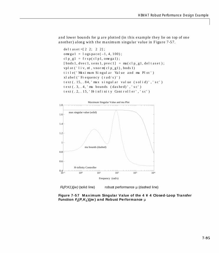
HIMAT Robust Performance Design Example
and lower bounds for µ are plotted (in this example they lie on top of oneanother) along with the maximum singular value in Figure 7-57.
deltaset=[2 2; 2 2];omega1 = logspace(–1,4,100);clp_g1 = frsp(clp1,omega1);[bnds1,dvec1,sens1,pvec1] = mu(clp_g1,deltaset);vplot('liv,m',vnorm(clp_g1),bnds1)title('Maximum Singular Value and mu Plot')xlabel('Frequency (rad/s)')text(.15,.84,'max singular value (solid)','sc')text(.3,.4,'mu bounds (dashed)','sc')text(.2,.15,'H-infinity Controller','sc')
Figure 7-57 Maximum Singular Value of the 4 ¥ 4 Closed-Loop Transfer Function FL(P,K1)(jw) and Robust Performance µ
0.4
0.6
0.8
1
1.2
1.4
1.6
1.8
10-1 100 101 102 103 104
max singular value (solid)
mu bounds (dashed)
H-infinity Controller
Maximum Singular Value and mu Plot
Frequency (rad/s)
FL(P,K1)(jw) (solid line) robust performance µ (dashed line)
7-95

7 Robust Control Examples
7-9
Hence, the controlled system (from H∞) does not achieve robust performance.This conclusion follows from the µ plot in Figure 7-57, which peaks to a valueof 1.69, at a frequency of 73.6 rad/sec. This means that there is a perturbationmatrix ∆G, with ||∆G||∞ = , for which the perturbed weighted sensitivity getslarge
||WP(I + Gnom(I + Wdel∆G)K–1||∞ = 1.69
This perturbation, ∆G, can be constructed using dypert. The input variables tothe command dypert consist of two outputs from µ, the perturbation matrixand the bounds, along with the block structure, and the numbers of the blocksfor which the rational matrix construction should be carried out. Often times,some of the blocks correspond to performance blocks and therefore need not beconstructed. Here, only the first block is an actual perturbation, so theconstruction is only done for this 2 × 2 perturbation (fourth argument ofdypert).
delta_G = dypert(pvec1,deltaset,bnds1,1);minfo(delta_G) % 2 by 2rifd(spoles(delta_G)) % stablehinfnorm(delta_G) % 1/1.69clp_pert = starp(delta_G,clp1,2,2); % close top loop with deltaminfo(clp_pert)rifd(spoles(clp_pert)) % stable, since RS passedhinfnorm(clp_pert) % degradation of performance
11.69-----------
e
-
clp1
delta G
d
e clp pert d
6
HIMAT Robust Performance Design Example
µ-Analysis of Loop Shape DesignRobust performance for the system with the loop shape controller, Kloop, canalso be analyzed using µ. You might think that the loop shaping controllerwould exhibit good robust performance properties, based on its excellentnominal performance and robust stability properties.
clpg = frsp(clp,omega1);bnds_loop = mu(clpg,deltaset);vplot('liv,m',bnds_loop)title('mu Plot of Closed-loop System')xlabel('Frequency (rad/s)')text(.6,.85,'Loop Shape Controller','sc')
However, the closed-loop system with the loop shaping controller does notachieve robust performance. In fact, µ reaches a peak value of 11.7 at afrequency of 0.202 rad/sec, as seen in Figure 7-58. This means that there is aperturbation matrix ∆G, with ||∆G||∞ = , for which the perturbed weightedsensitivity gets large
||WP(I + Gnom(I + Wdel∆G)K–1||∞ = 11.7
Notice that this perturbation is 8.2 times smaller than the perturbationassociated with the H∞ control design, but that the subsequent degradation inclosed-loop performance is 8.2 times worse. Therefore, the loop shapingcontroller will most likely perform poorly on the real system.
111.7-----------
7-97

7 Robust Control Examples
7-9
Figure 7-58 Robust Performance µ Plot of the Closed-Loop HIMAT System with the Loop Shaping Controller
The structured singular value µ is large in the low frequency range due to theoff-diagonal elements of clpg being large. One can see this using the commandblknorm, which outputs the individual norms of the respective blocks. Thecoupling between the off-diagonal terms associated with 0.202 rads/sec point tothe problem — the upper right entry is 0.14, somewhat small, but not small
0
2
4
6
8
10
12
10-1 100 101 102 103 104
Loop Shape Controller
Frequency (rad/s)
mu Plot of Closed-loop System
8

HIMAT Robust Performance Design Example
enough to counteract the large (nearly 1000) lower left entry. As expected,.
blkn_cl = blknorm(clpg,deltaset);see(xtract(blkn_cl,.15,.3))
2 rows 2 columns
iv = 0.1599864.9995e-01 1.4127e-015.6525e+02 1.6402e-01
iv = 0.2023594.9991e-01 1.4193e-019.5950e+02 1.6520e-01
iv = 0.2559554.9985e-01 1.4294e-017.5635e+02 1.6607e-01
Recapping ResultsLet's summarize what has been done so far:
• The generalized plant, himat_ic, which includes the aircraft model,uncertainty and performance weighting functions, and the interconnectionof all of these components was built using sysic.
• A controller was designed using hinfsyn.
• The robust performance characteristics of the closed-loop system wereanalyzed with a structured singular value frequency domain test using mu.
The structured singular value analysis involved computing µ at each frequencyof this 4 × 4 closed loop response, with respect to a block structure ∆ which ismade up of two 2 × 2 full blocks. The blocks represent, respectively, uncertaintyin the aircraft model, and the performance objectives.
At this stage, the controller which has been designed using H∞ techniques(nearly) minimizes the H∞ norm of the closed loop transfer function from the4 × 1 vector of perturbation inputs and disturbance inputs to the 4 × 1 vectorof perturbation outputs and error signals. The structured singular value
µ 0.14*959 11.6=≈
7-99

7 Robust Control Examples
7-1
analysis shows that the µ analysis improves on the bound at mostfrequencies, but there is no improvement at the frequency of 73.6 rads/sec.
Hence, the peak value of the µ-plot is as high as the peak value on the singularvalue plot, the µ analysis seems to have been of little use. However, at most ofthe frequencies, µ is smaller than , and in the next iteration of synthesis, thecontroller can essentially focus its efforts at the problem frequency, and lowerthe peak of the µ-plot.
D – K Iteration for HIMAT Using dkitThe µ-Tools M-file dkit automates the µ-synthesis procedure via D – Kiteration. This example is a modified version of the HIMAT problem consideredearlier (see Figure 7-47) and is extended to include a frequency dependentsensor noise signal, as shown in the closed-loop interconnection diagram inFigure 7-59. This sensor noise signal is included to represent a more realisticperformance objective.
Figure 7-59 HIMAT Closed-Loop Interconnection Structure
Now, the open-loop interconnection structure is the eight input, six outputlinear system, shown below
with internal structure, as in Figure 7-60.
σ .( )
σ
pertinz
diste
controly
himat ic
00

HIMAT Robust Performance Design Example
The M-file mkhicn creates the plant model, weighting functions and theinterconnection structure shown in Figure 7-60. This can be produced withnine MATLAB commands, listed below, and also in the M-file mkhicn (whichcreates the plant and weighting functions).
Figure 7-60 HIMAT Open-Loop Interconnection Structure
mkhicn
file: mkhicn.mmkhimat;wdel = nd2sys([50 5000],[1 10000]);wp = nd2sys([0.5 0.9],[1 0.018]);poleloc = 320;Wn = nd2sys([2 0.008*poleloc],[1 poleloc]);wdel = daug(wdel,wdel);wp = daug(wp,wp);Wn = daug(wn,wn);
systemnames = ' himat wp wdel wn ';inputvar = '[ pertin2 ; dist4 ; control2 ]';outputvar = '[ wdel ; wp ; himat + dist(1:2) + wn ]';input_to_himat = '[ control + pertin ]';input_to_wdel = '[ control ]';input_to_wp = '[ himat + dist(1:2) ]';input_to_wn = '[ dist(3:4) ]';sysoutname = 'himat_ic';cleanupsysic = 'yes';
sysic;
"e1
e2
#
control?
dist(3:4)wnf ++
y
f++
- - - f++
- -
pertin dist(1:2)
"w1
w2
#
6
6
? ?
wdel
wphimat
7-101

7 Robust Control Examples
7-1
The dkit file himat_dk has been set up with the necessary variables to designrobust controllers for HIMAT using D – K iteration. A listing of the himat_dkfile follows. You can copy this file into your directory from the µ-Toolssubroutines directory, mutools/subs, and modify it for other problems, asappropriate.
% himat_dk%% This script file contains the USER DEFINED VARIABLES for the %mutools DKIT script file. The user MUST define the 5 %variables below.%------------------------------------------%
REQUIRED USER DEFINED VARIABLES%------------------------------------------%% Nominal plant interconnection structureNOMINAL_DK = himat_ic;
% Number of measurementsNMEAS_DK = 2;
% Number of control inputsNCONT_DK = 2;
% Block structure for mu calculationBLK_DK = [2 2;4 2];
% Frequency response rangeOMEGA_DK = logspace(–3,3,60);
%----------------------end of himat_dk-------------------------%
02

HIMAT Robust Performance Design Example
After the himat_dk.m file has been set up, you need to let the dkit programknow which setup file to use. This is done by setting the string variableDK_DEF_NAME in the MATLAB workspace equal to the setup filename. Typingdkit at the MATLAB prompt will then begin the D – K iteration procedure.
DK_DEF_NAME = 'himat_dk';dkitstarting mu iteration #: 1
Iteration Number: 1-------------------
Information about the Interconnection Structure IC_DK:system10 states 6 outputs8 inputsTest bounds: 0.0000 < gamma <= 100.0000
Gamma value achieved: 2.1516
gamma hamx_eig xinf_eig hamy_eig yinf_eig nrho_xy p/f
100.000 2.3e-02 0.0e+00 1.8e-02 0.0e+00 0.0003 p
50.000 2.3e-02 0.0e+00 1.8e-02 0.0e+00 0.0011 p
25.000 2.3e-02 0.0e+00 1.8e-02 0.0e+00 0.0046 p
12.500 2.3e-02 0.0e+00 1.8e-02 0.0e+00 0.0183 p
6.250 2.3e-02 0.0e+00 1.8e-02 0.0e+00 0.0742 p
3.125 2.3e-02 0.0e+00 1.8e-02 0.0e+00 0.3117 p
1.562 2.3e-02 0.0e+00 1.7e-02 0.0e+00 1.5583# f
2.152 2.3e-02 0.0e+00 1.8e-02 0.0e+00 0.7100 p
7-103

7 Robust Control Examples
7-1
Singular Value plot of closed-loop system in GRAPHICS windowMake sure that chosen Frequency range is appropriate
0
0.2
0.4
0.6
0.8
1
1.2
1.4
1.6
1.8
2
10-3 10-2 10-1 100 101 102 103
SINGULAR VALUE PLOT: CLOSED-LOOP RESPONSE
FREQUENCY (rad/s)
MA
GN
ITU
DE
04

HIMAT Robust Performance Design Example
Next, we get to change the frequency range, if desired. For illustrativepurposes, we will change the number of logarithmically spaced points from 60to 70.
Do you want to modify OMEGA_DK? (y/n): y
Current Frequency Variable---------------------------------------------------------------(s)Frequency Spacinglog(n) # Frequency Points60(b)Frequency - bottom1.00e–03(h)Frequency - high1.00e+03
Enter (s n b and/or h) to change OMEGA, (e) to exit unchanged: n
------------CHANGING # of Points--------------
Enter desired # of points: 70
Current Frequency Variable---------------------------------------------------------------(s)Frequency Spacinglog(n) # Frequency Points70(b)Frequency - bottom1.00e–03(h)Frequency - high1000
Enter (s n b and/or h) to change, (e) to exit: e
By typing e, we exit the frequency range modification, and the closed-loopsingular value frequency response is recalculated and plotted. In this case, theplot looks exactly the same.
7-105

7 Robust Control Examples
7-1
Singular Value plot of closed-loop system in GRAPHICS windowMake sure that chosen Frequency range is appropriate
Do you want to modify OMEGA_DK? (y/n): n
RERUN H_inf with DIFFERENT bounds/tolerances? (y/n): n
Calculating MU of closed-loop system: g_dkpoints completed....1.2.3.4.5.6.7.8.9.10.11.12.13.14.15.16.17.18.19.20.21.22.23.24.25.26.27.28.29.30.31.32.33.34.35.36.37.38.39.40.41.42.43.44.45.46.47.48.49.50.51.52.53 .54.55.56.57.58.59.60.61.62.63.64.65.66.67.68.69.70.
0
0.2
0.4
0.6
0.8
1
1.2
1.4
1.6
1.8
2
10-3 10-2 10-1 100 101 102 103
SINGULAR VALUE PLOT: CLOSED-LOOP RESPONSE
FREQUENCY (rad/s)
MA
GN
ITU
DE
06

HIMAT Robust Performance Design Example
MU plot for control design:Press any key to continue
Iteration Summary------------------------------------Iteration #1Controller Order10Total D-Scale Order0Gamma Achieved2.152Peak mu-Value2.075
Another D–K itera;tion? (y/n): y
Proceeding with the D – K iteration, we must fit the D-scaling variable that wascalculated in the µ upper-bound computation. This rational D-scaling will thenbe absorbed into the open-loop interconnection.
0.4
0.6
0.8
1
1.2
1.4
1.6
1.8
2
10-3 10-2 10-1 100 101 102 103
CLOSED-LOOP MU: CONTROLLER #1
FREQUENCY (rad/s)
MU
7-107

7 Robust Control Examples
7-1
A plot of the µ upper bound, the first frequency-dependent D-scaling data (thisis the curve we want to fit), and the sensitivity of the µ upper bound. Thesensitivity measure roughly shows (across frequency) the relative importanceof the accuracy of the curve fit. It is used in the curve fit optimization to weightsome frequency ranges differently than others.
105
100
105
0.5
1
1.5
2
2.5MU Upper Bound
105
100
105
101
100
101
Magnitude Data: (1;1 1:d)
105
100
105
101
100
101
Sensitivity
08

HIMAT Robust Performance Design Example
You are prompted to enter your choice of options for fitting the D-scaling data.Press return to see your options.
Enter Choice (return for list):Choices:
• nd and nb allow you to move from one D-scale data to another. nd moves tothe next scaling, whereas nb moves to the next scaling block. For scalarD-scalings, these are identical operations, but for problems with fullD-scalings, (perturbations of the form δI) they are different. In the (1,2)subplot window, the title displays the D-scaling Block number, the row/column of the scaling that is currently being fit, and the order of the currentfit (with d for data, when no fit exists).
• The order of the current fit can be incremented or decremented (by 1) usingi and d.
• apf automatically fits each D-scaling data. The default maximum state orderof individual D-scaling is 5. The mx variable allows you to change themaximum D-scaling state order used in the automatic pre-fitting routine. mxmust be a positive, nonzero integer. at allows you to define how close therational, scaled µ upper bound is to approximate the actual µ upper bound ina norm sense. Setting at 1 would require an exact fit of the D-scale data, andis not allowed. Allowable values are greater than 1, and the meaning is
nd Move to Next D-Scaling
nb Move to Next D-Block
i Increment Fit Order
d Decrement Fit Order
apf Auto-PreFit
mx 3 Change Max-Order to 3
at 1.01 Change Auto-PreFit Tol to 1.01
0 Fit with zeroth order
2 Fit with second order
n Fit with n'th order
e Exit with Current Fittings
s See Status
7-109

7 Robust Control Examples
7-1
explained in Chapter 5, “Control Design via µ Synthesis”. This setting playsa role (mildly unpredictable, unfortunately) in determining where in the(D,K) space the D – K iteration converges.
• Entering a positive integer at the prompt will fit the current D-scale datawith that state order rational transfer function.
• e exits the D-scale fitting to continue the D – K iteration.
• The variable s will display a status of the current and fits.
Select apf to automatically fit the D-scale data. After a few seconds ofcalculation, the first D-scale is fit with a fourth order rational curve as shownin the top-right plot, along with the frequency-dependent magnitude data thatis being fit. Also shown in the top-left portion of the graphics window is a plotcomparing the upper bound of µ (using the frequency dependent D-scalings)along with the maximum singular value of the closed-loop transfer functionafter being scaled by the just-computed rational fit. Note that the secondD-scale data, which corresponds to the performance block, is fit with aconstant. This is expected since one of the D-scalings can always be normalizedto be 1. Enter s after the D-scale fitting is completed to see the status.
Enter Choice (return for list): apfStarting Auto-PreFit...Block 1 , Order = 0 1 2 3 4Block 2 , Order = 0
Done
Enter Choice (return for list): s
Block 1: 4Block 2: 0Auto PreFit Fit Tolerance: 1.03Auto PreFit Maximum Order: 5
Enter Choice (return for list):
10

HIMAT Robust Performance Design Example
In this case, the µ upper bound with the D-scale data is very close to the µ upperbound with the rational D-scale fit. The fourth order fit is quite adequate inscaling the closed-loop transfer function. The curve fitting procedure for thisscaling variable is concluded by entering e at the Enter Choice prompt.
Enter Choice (return for list): e
In this problem, the block structure consists of two complex full blocks: the2 × 2 block associated with the multiplicative uncertainty model for theaircraft, and the 4 × 2 performance block. Since there are two blocks, thereis only one D-scaling variable, and we are completely done with the curvefitting in this iteration.
105
100
105
0.5
1
1.5
2
2.5Scaled Bound and MU
105
100
105
101
100
101
Magnitude Data and Fit: (1;1 1:4)
105
100
105
101
100
101
Sensitivity
7-111
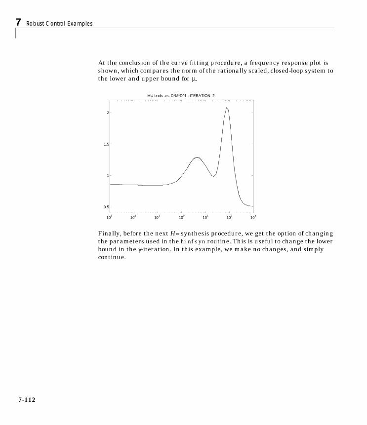
7 Robust Control Examples
7-1
At the conclusion of the curve fitting procedure, a frequency response plot isshown, which compares the norm of the rationally scaled, closed-loop system tothe lower and upper bound for µ.
Finally, before the next H∞ synthesis procedure, we get the option of changingthe parameters used in the hinfsyn routine. This is useful to change the lowerbound in the γ-iteration. In this example, we make no changes, and simplycontinue.
103
102
101
100
101
102
103
0.5
1
1.5
2
MU bnds .vs. D*M*D^1 : ITERATION 2
12

HIMAT Robust Performance Design Example
Altering the HINFSYN settings for next synthesis...
HINFSYN Settings Previously Next------------------------------------------------------------(u)GAMMA Upper Bound100 2.146(l)GAMMA Lower Bound 0.00e+000.00e+00(t)Bisection Tolerance1.0004.29e–02(p)Riccati PSD epsilonl.00e–06l.00e–06(j)Riccati j–w epsilonl.00e–08l.00e–08
Enter (u l t p j) to change, (e) to exit: e
The iteration proceeds by computing the H∞ optimal controller for the scaled(using the rational scalings from the curve fitting) open-loop system.
Iteration Number: 2--------------------
Information about the Interconnection Structure IC_DK:system:26 states6 outputs8 inputsTest bounds: 0.0000 < gamma <= 2.1461
Gamma value achieved:1.0730
gamma hamx_eig xinf_eig hamy_eig yinf_eig nrho_xy p/f
2.146 2.Oe–02 –5.2e–14 1.8e–02 –1.5e–16 0.1557 p
1.073 1.9e–02 –4.6e–14 1.7e–02 –3.4e–17 0.9958 p
0.537 1.4e–14# ******* 1.2e–02 –1.7e–18 ****** f
0.805 1.8e–02 –7.7e–13 1.6e–02 –5.8e–18 4.9336# f
1.019 1.9e–02 –6.Oe–14 1.7e–02 –2.4e–17 1.2077# f
1.055 1.9e–02 –2.3e–13 1.7e–02 –3.8e–17 1.0589# f
7-113
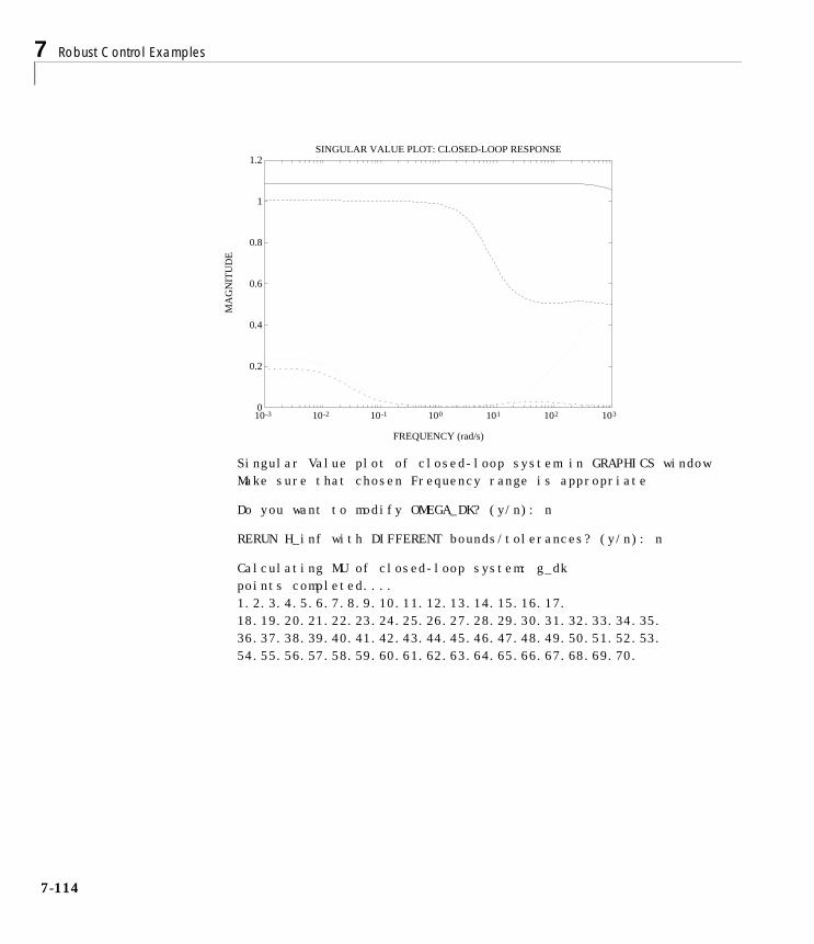
7 Robust Control Examples
7-1
Singular Value plot of closed-loop system in GRAPHICS windowMake sure that chosen Frequency range is appropriate
Do you want to modify OMEGA_DK? (y/n): n
RERUN H_inf with DIFFERENT bounds/tolerances? (y/n): n
Calculating MU of closed-loop system: g_dkpoints completed....1.2.3.4.5.6.7.8.9.10.11.12.13.14.15.16.17.18.19.20.21.22.23.24.25.26.27.28.29.30.31.32.33.34.35.36.37.38.39.40.41.42.43.44.45.46.47.48.49.50.51.52.53.54.55.56.57.58.59.60.61.62.63.64.65.66.67.68.69.70.
0
0.2
0.4
0.6
0.8
1
1.2
10-3 10-2 10-1 100 101 102 103
SINGULAR VALUE PLOT: CLOSED-LOOP RESPONSE
FREQUENCY (rad/s)
MA
GN
ITU
DE
14

HIMAT Robust Performance Design Example
MU plot for control design:Press any key to continue
Iteration Summary--------------------------------------------Iteration #12Controller Order1026Total D-Scale Order016Gamma Achieved2.1521.073Peak mu-Value2.0751.073
Another D–K iteration? (y/n): y
The third iteration begins by fitting the new frequency-dependent D-scaling.
0.5
0.6
0.7
0.8
0.9
1
1.1
10-3 10-2 10-1 100 101 102 103
CLOSED-LOOP MU: CONTROLLER #2
FREQUENCY (rad/s)
MU
7-115

7 Robust Control Examples
7-1
Again, enter the automatic pre-fitting option apf.
Enter Choice (return for list): apfStarting Auto-PreFit...Block 1 , Order = 0 1 2 3 4 5Block 2 , Order = 0Done
105
100
105
0.6
0.8
1
1.2MU Upper Bound
105
100
105
102
101
100
101
Magnitude Data: (1;1 1:d)
105
100
105
101
100
101
Sensitivity
16

HIMAT Robust Performance Design Example
This fifth order fit works well in scaling the transfer function, so we exit thecurve fitting routine.
Enter Choice (return for list):e
105
100
105
0.6
0.8
1
1.2Scaled Bound and MU
105
100
105
102
101
100
101
Magnitude Data and Fit: (1;1 1:5)
105
100
105
101
100
101
Sensitivity
103
102
101
100
101
102
103
0.6
0.7
0.8
0.9
1
1.1MU bnds .vs. D*M*D^1 : ITERATION 3
7-117
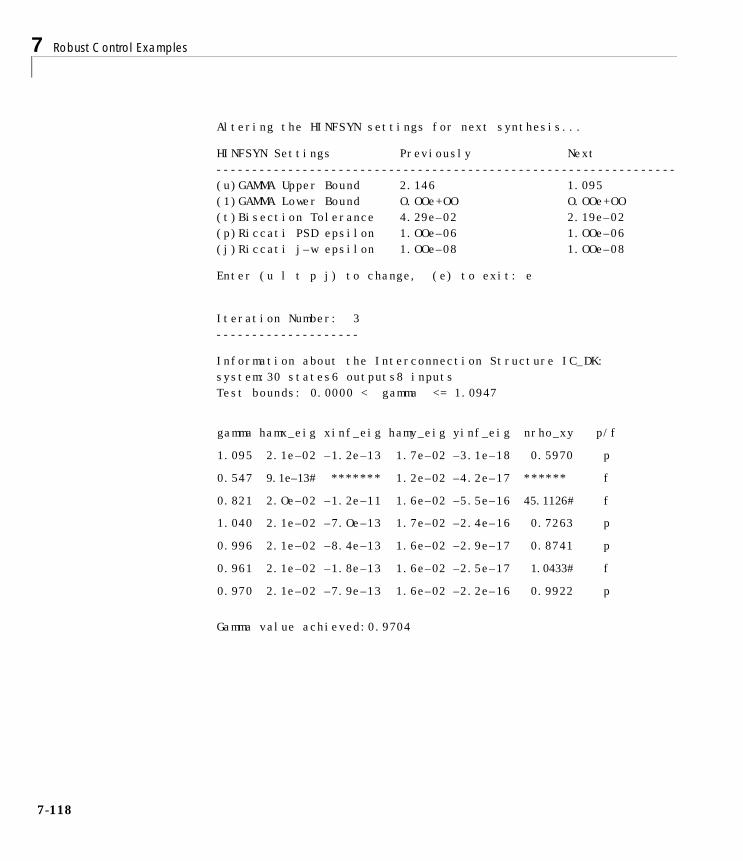
7 Robust Control Examples
7-1
Altering the HINFSYN settings for next synthesis...
HINFSYN Settings Previously Next----------------------------------------------------------------(u)GAMMA Upper Bound 2.146 1.095(1)GAMMA Lower Bound O.OOe+OO O.OOe+OO(t)Bisection Tolerance 4.29e–02 2.19e–02(p)Riccati PSD epsilon 1.OOe–06 1.OOe–06(j)Riccati j–w epsilon 1.OOe–08 1.OOe–08
Enter (u l t p j) to change, (e) to exit: e
Iteration Number: 3--------------------
Information about the Interconnection Structure IC_DK:system:30 states6 outputs8 inputsTest bounds: 0.0000 < gamma <= 1.0947
Gamma value achieved:0.9704
gamma hamx_eig xinf_eig hamy_eig yinf_eig nrho_xy p/f
1.095 2.1e–02 –1.2e–13 1.7e–02 –3.1e–18 0.5970 p
0.547 9.1e–13# ******* 1.2e–02 –4.2e–17 ****** f
0.821 2.Oe–02 –1.2e–11 1.6e–02 –5.5e–16 45.1126# f
1.040 2.1e–02 –7.Oe–13 1.7e–02 –2.4e–16 0.7263 p
0.996 2.1e–02 –8.4e–13 1.6e–02 –2.9e–17 0.8741 p
0.961 2.1e–02 –1.8e–13 1.6e–02 –2.5e–17 1.0433# f
0.970 2.1e–02 –7.9e–13 1.6e–02 –2.2e–16 0.9922 p
18

HIMAT Robust Performance Design Example
Singular Value plot of closed-loop system in GRAPHICS window. Make surethat chosen Frequency range is appropriate
Do you want to modify OMEGA_DK? (y/n): n
RERUN H_inf with DIFFERENT bounds/tolerances? (y/n): n
Calculating MU of closed-loop system: g_dkpoints completed....1.2.3.4.5.6.7.8.9.10.11.12.13.14.15.16.17.18.19.20.21.22.23.24.25.26.27.28.29.30.31.32.33.34.35.36.37.38.39.40.41.42.43.44.45.46.47.48.49.50.51.52.53.54.55.56.57.58.59.60.61.62.63.64.65.66.67.68.69.70.
0
0.1
0.2
0.3
0.4
0.5
0.6
0.7
0.8
0.9
1
10-3 10-2 10-1 100 101 102 103
SINGULAR VALUE PLOT: CLOSED-LOOP RESPONSE
FREQUENCY (rad/s)
MA
GN
ITU
DE
7-119

7 Robust Control Examples
7-1
MU plot for control design:Press any key to continue
Iteration Summary----------------------------------------------------------Iteration #123Controller Order102630Total D-Scale Order01620Gamma Achieved2.1521.0730.970Peak mu-Value2.0751.0730.973
Another D–K itera;tion? (y/n): necho offNext MU iteration number: 4
At this point, we have achieved the robust performance objective, and we endthe D – K iteration. We have designed a 30 state controller using D – Kiteration which achieves a µ value less than 1.
In this example, it is also possible to reduce the controller order to 12, usingtruncated balanced realizations, and still maintain closed-loop stability androbust performance.
103
102
101
100
101
102
103
0.6
0.65
0.7
0.75
0.8
0.85
0.9
0.95
1CLOSEDLOOP MU: CONTROLLER #3
FREQUENCY (rad/s)
MU
20

HIMAT Robust Performance Design Example
max(real(spoles(kd_k3)))
ans =–1.6401e–02
[k_dk3bal,hsv] = sysbal(k_dk3);[k_dk3red] = strunc(k_dk3bal,12);clpred_12 = starp(himat_ic,k_dk3red);max(real(spoles(clpred_12)))
ans =–6.9102e–03
clpred_12g = frsp(clpred_12,OMEGA_DK);[bnds] = mu(clpred_12g,[2 2;4 2],'c');pkvnorm(sel(bnds,1,1))
ans =9.9910e–01
H∞ Loop Shaping Design for HIMATNow consider H∞ loop shaping control design for the HIMAT example discussedin previous sections. Recall that the objective is to reject disturbances up toabout 1 rad/sec in the presence of substantial plant uncertainty above 100 rad/sec. A loop-shaping design that gives a bandwidth of approximately 10 rad/secand robustness which should be satisfactory.
Design PrecompensatorFirst form the HIMAT system and plot its maximum singular values acrossfrequency (see Figure 7-61).
mkhimat[type,p,m,n] = minfo(himat);om = logspace(–2,4,100);himatg = frsp(himat,om);vplot('liv,lm',vsvd(himatg),1);title('SINGULAR VALUES OF HIMAT')ylabel('SINGULAR VALUES'); xlabel('FREQUENCY (RAD/SEC)');
7-121

7 Robust Control Examples
7-1
Figure 7-61 Singular Values of HIMAT
The singular values of himat are plotted in Figure 7-61, and although the unitygain cross over frequency is approximately correct, the low frequency gain istoo low. We therefore introduce a proportional plus integral (P+I)precompensator with transfer function (1 + s–1)I2×2 to boost the low frequencygain and give zero steady state errors. The singular values of himat and himataugmented with the P+I compensator are shown in Figure 7-62.
sysW1 = daug(nd2sys([1 1],[1 0]),nd2sys([1 1],[1 0]));sysGW = mmult(himat,sysW1);sysGWg = frsp(sysGW,om);vplot('liv,lm',vsvd(himatg),'-.',vsvd(sysGWg),'-',1,'--')title('SINGULAR VALUES OF HIMAT AND AUGMENTED HIMAT')ylabel('SINGULAR VALUES');xlabel('FREQUENCY (RAD/SEC)');
10-3
10-2
10-1
100
101
102
103
104
105
10-2 10-1 100 101 102 103 104
SINGULAR VALUES OF HIMAT
FREQUENCY (RAD/SEC)
SIN
GU
LAR
VA
LUE
S
22
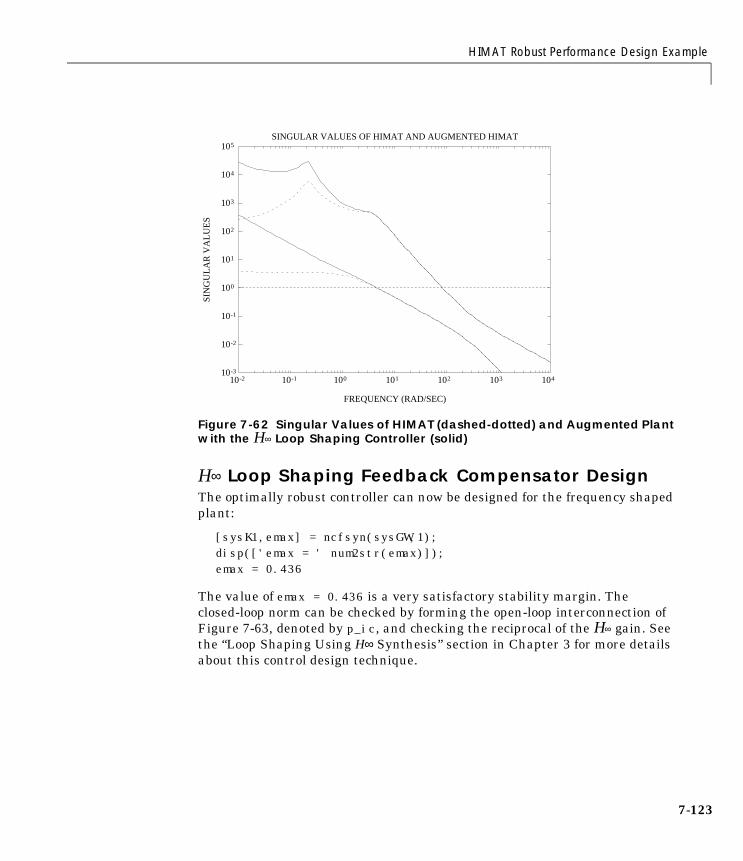
HIMAT Robust Performance Design Example
Figure 7-62 Singular Values of HIMAT (dashed-dotted) and Augmented Plant with the H∞ Loop Shaping Controller (solid)
H∞ Loop Shaping Feedback Compensator DesignThe optimally robust controller can now be designed for the frequency shapedplant:
[sysK1,emax] = ncfsyn(sysGW,1);disp(['emax = ' num2str(emax)]);emax = 0.436
The value of emax = 0.436 is a very satisfactory stability margin. Theclosed-loop norm can be checked by forming the open-loop interconnection ofFigure 7-63, denoted by p_ic, and checking the reciprocal of the H∞ gain. Seethe “Loop Shaping Using H∞ Synthesis” section in Chapter 3 for more detailsabout this control design technique.
10-3
10-2
10-1
100
101
102
103
104
105
10-2 10-1 100 101 102 103 104
SINGULAR VALUES OF HIMAT AND AUGMENTED HIMAT
FREQUENCY (RAD/SEC)
SIN
GU
LAR
VA
LUE
S
7-123

7 Robust Control Examples
7-1
Figure 7-63 H∞ Loop Shaping Standard Block Diagram
systemnames = 'sysGw';inputvar = '[ w12; w22; u2 ]';outputvar = '[ u; w1+sysGw; w1+sysGw ]';input_to_sysGw = '[ w2+u ]';sysoutname = 'p_ic';cleanupsysic = 'yes';sysic;ncf_cl = starp(p_ic,sysK1);ncf_cl_nm = hinfnorm(ncf_cl);1/ncf_cl_nm(1)ans =
4.3598e–01The implemented controller involves the pre- and postweighting functions W1and W2, as shown in Figure 7-64.
Figure 7-64 Actual Implemented H∞ Loop Shaping Controller
24

HIMAT Robust Performance Design Example
In this example W2 = I2×2, therefore, the implemented loop shaping controlleris:
sysKloop = mmult(sysW1,sysK1);
Assessing Robust Performance with µWe can now assess this controller by testing the original specification by usinga µ-test as in previous designs. First the interconnection structure needs to beformed.
wdel = nd2sys([50,5000],[1,10000]);wp = nd2sys([0.5,1.5],[1,0.03]);wdel = daug(wdel,wdel);wp = daug(wp,wp); himaticclear wp wdel
Now form the closed-loop and evaluate the robust performance µ with the H∞
loop shaping compensator implemented (see Figure 7-65).
clp1 = starp(himat_ic,sysKloop,2,2);clp_g1 = frsp(clp1,om);deltaset = [2 2; 2 2];[bnds1,dvec1,sens1,pvec1] = mu(clp_g1,deltaset);vplot('liv,m',bnds1);title('ROBUST PERFORMANCE MU WITH LOOPSHAPE CONTROLLER')ylabel('MU');xlabel('FREQUENCY (RAD/SEC)');disp(['mu value is ' num2str(pkvnorm(sel(bnds1,1,1)))])mu value is 1.323
7-125

7 Robust Control Examples
7-1
Figure 7-65 Robust Performance µ with sysK1
The plot of µ is shown in Figure 7-65 (solid line), the µ-value is close to thatrequired, giving a satisfactory design without exploiting the details of theperformance and uncertainty weights. This substantiates the claim that thisdesign method can give a very robust initial design which does not requiredetailed trade-offs between weights to be studied.
Reduced Order DesignsThe previously designed controller will typically have one less state than theprecompensator plus the plant. It is therefore often desirable to reduce thenumber of states in the controller. There are systematic techniques for doingthis based on model reduction in the ν gap metric, δν, which is roughlyequivalent to model reduction of normalized coprime factors of the plant andcontroller.
0
0.2
0.4
0.6
0.8
1
1.2
1.4
10-2 10-1 100 101 102 103 104
ROBUST PERFORMANCE MU WITH LOOPSHAPE CONTROLLER
FREQUENCY (RAD/SEC)
MU
26

HIMAT Robust Performance Design Example
First reduce the weighted plant model order and measure the resulting gap.
[sysGW_cf,sigGW]=sncfbal(sysGW);sigGWsigGW =
8.9996e–017.1355e–013.3542e–017.9274e–028.5314e–042.1532e–04
sysGW_4 = cf2sys(hankmr(sysGW_cf,sigGW,4,'d'));gapGW_4 = nugap(sysGW,sysGW_4)gapGW_4 =
8.6871e–04
It is seen that a fourth order model is essentially indistinguishable from thefull order model due to the small value of the ν gap. Now design the controllerfor this reduced order system.
[sysK1_3,emax_3] = ncfsyn(sysGW_4,1);emax_3emax_3 =
4.3597e–01This three state controller can be reduced to two states using Hankel modelreduction techniques (hankmr).
[sysK1_3_cf,sigK1_3] = sncfbal(sysK1_3);sigK1_3sigK1_3 =
3.1674e–012.7851e–016.9959e–02
sysK1_2 = cf2sys(hankmr(sysK1_3_cf,sigK1_3,2,'d'));gapK_2=nugap(sysK1_3,sysK1_2)gapK_2 =
6.9959e–02
7-127

7 Robust Control Examples
7-1
The robustness bound in the “Loop Shaping Using H∞ Synthesis” section inChapter 3, equation (3-23), can now be applied to give a lower bound onrobustness,
e_bound=sin(asin(emax_3)-asin(gapGW_4)-asin(gapK_2))e_bound =
3.7114e–01
and this can be compared with the actual stability margin with the reducedorder controller as follows:
cl_red = starp(p_ic,sysK1_2);tmp = hinfnorm(cl_red);e_act=1/tmp(1)e_act =
4.0786e–01
It is seen that the actual robustness is about half way between the optimal andthis lower bound. The important use of the bounds is that they indicate whatlevel of reduction is guaranteed not to degrade robustness significantly.
This gives a third-order controller together with the second-order P+I term.The µ-value for this controller, not shown here, turns out to have essentiallythe same µ -value as the closed-loop system with the full order controller.
Introducing a Reference SignalA reference signal can be introduced into the loop shaping control design asfollows.
[sysK3,emax] = ncfsyn(sysGW,1.1,'ref');cl_ref = starp(p_ic,sysK3,2,2);minfo(cl_ref)system: 12 states 4 outputs 6 inputs
When the ncfsyn option ref is specified, the controller includes an extra set ofreference inputs. The second input argument to ncfsyn is 1.1. This implies weare designing a suboptimal controller with 10% less performance than at theoptimal. In practice, a 10% suboptimal design often performs better in terms ofrobust performance than the optimal controller on the actual system.
28
HIMAT Robust Performance Design Example
The last two inputs to cl_ref correspond to the reference signals, the first twooutputs are the outputs of the controller and the last two outputs are the inputsto the controller (plant output plus observation noise). This design makes theclosed-loop transfer function from reference to plant output the numerator of anormalized coprime factorization of sysGW. An external reference compensatorcould also be added to improve the command response and there are manypossibilities. Here we first diagonalize the closed-loop reference to outputtransfer function and then insert some phase advance to increase the speed ofresponse.
cl_ref_yr=sel(cl_ref,3:4,5:6);P0 = transp(mmult([0 1; –1 0],cl_ref_yr,[0 1; –1 0]));P1 = nd2sys([10 50],[1 50]);P2 = daug(P1,P1);sysQ = mmult(P0,P2);
Now reduce the order of sysQ to four states using the balanced realizationtechnique (sysbal), and incorporate into the controller.
[sysQ_b,sig_Q] = sysbal(sysQ);sig_Qsig_Q =
3.9665e+002.9126e+007.2360e–014.5915e–012.3600e–021.0016e–021.2526e–065.2197e–07
sysQ4 = strunc(sysQ_b,4);sysK_ref = mmult(sysK3,daug(eye(2),sysQ4));
Finally form the closed-loop and calculate the step response.
sys_cl_ref = starp(p_ic,sysK_ref,2,2);y = trsp(sys_cl_ref,[0;0;0;0;1;0],0.5,.001);vplot(sel(y,1,1),'-.',sel(y,2,1),'.',sel(y,3,1),'-',...
sel(y,4,1),'--')title('CLOSED LOOP TIME RESPONSE WITH SYSK1')xlabel('TIME (SECONDS)')
7-129

7 Robust Control Examples
7-1
The step responses are plotted in Figure 7-66. The first output (solid) tracks thecommand well with a rise time of less than 0.1 second and no overshoot. Theoutput of the second channel (dashed) is zero, indicating that there is no crosscoupling between the output channels in the nominal closed-loop system. Thecontroller output commands (dotted and dashed-dotted lines) are also plotted.This is just the nominal step response and further tests are needed to check thesensitivity of the closed-loop to the plant uncertainty.
Figure 7-66 Time Response of Closed Loop System: sysK1
-3.5
-3
-2.5
-2
-1.5
-1
-0.5
0
0.5
1
0 0.05 0.1 0.15 0.2 0.25 0.3 0.35 0.4 0.45 0.5
..................................
................................................................
...................................................................................................................................................................................................................................................................................................................................................................................................................
CLOSED LOOP TIME RESPONSE WITH SYSK1
TIME (SECONDS)
30

HIMAT Robust Performance Design Example
HIMAT ReferencesFreudenberg, J., and D. Looze, “Frequency domain properties of scalar andmultivariable feedback systems,” Lecture Notes in Control and InformationSciences, Springer-Verlag, 1988.
Hartman, G.L., M.F. Barrett and C.S. Greene, “Control designs for an unstablevehicle,” NASA Dryden Flight Research Center, Contract Report NAS 4–2578,December, 1979.
Merkel, P.A., and R.A. Whitmoyer, “Development and evaluation of precisioncontrol modes for fighter aircraft,” Proceedings of the AIAA Guidance andControl Conference, San Diego, CA, Paper 76–1950, 1976.
Safonov, M.G., A.J. Laub, and G.L. Hartman, “Feedback properties ofmultivariable systems: The role and use of the return difference matrix,” IEEETransactions on Automatic Control, Vol. AC–26, No. 1, pp. 47–65, February,1981.
7-131

7 Robust Control Examples
7-1
F–14 Lateral-directional Control DesignConsider the design of a lateral-directional axis controller for the F–14 aircraftduring powered-approach to landing. The linearized F–14 model is found at anangle-of-attack (α) of 10.5 degrees and airspeed of 140 knots. The controlproblem is posed as a robust performance, model matching problem withmultiplicative plant uncertainty at the plant input and minimization ofweighted output transfer functions as the performance criterion. A diagram forthe closed-loop system, which includes the feedback structure of the plant andcontroller, and elements associated with the uncertainty models andperformance objectives, is shown in Figure 7-67.
Figure 7-67 F-14 Control Block Diagram
The performance objective is to have the true airplane, represented by thedashed box in Figure 7-67, respond effectively to the pilot's lateral stick andrudder pedal inputs. These performance objectives include:
32

F–14 Lateral-directional Control Design
• Decoupled response of the lateral stick, δlstk, to roll rate, p, and rudderpedals, δrudp, to side-slip angle, β. The lateral stick and rudder pedals havea maximum deflection of ± 1 inch. Therefore, they are represented asunweighted signals in Figure 7-67.
• The aircraft handling quality (HQ) response from the lateral stick to roll rate
should be a first order system, . The aircraft handling quality
response from the rudder pedals to side-slip angle should be
.
hqmod_p = nd2sys(5,[1 2]);hqmod_beta = nd2sys(1.25^2,[1 2.5 1.25^2],–2.5);
The stabilizer actuators have ±20 degs and ±90 degs/sec deflection anddeflection rate limits. The rudder actuators have ±30 degs and ±125 degs/secdeflection and deflection rate limits.
• The three measurement signals — roll rate, yaw rate, and lateralacceleration —are passed through second order, anti-aliasing filters prior tobeing fed to the controller.
• The natural frequency, ω, and damping, ζ, values for the yaw rate and lateralacceleration filters are 12.5Hz and 0.5, respectively, and 4.1 Hz and 0.7 forthe roll rate filter. The anti-aliasing filters have unity gain at DC (see Figure7-67). These signals are also corrupted by noise prior to entering thecontroller.
5 2s 2+------------
deg sec⁄inch
----------------------
2.5– 1.252
s2 2.5s 1.252
+ +--------------------------------------------- deg sec⁄
inch----------------------
anti-aliasing filter ω2
s2 2ζω ω2+ +
------------------------------------=
7-133

7 Robust Control Examples
7-1
freq = 12.5;fr = freq*2*pi;zeta = 0.5;antiaf_yaw = nd2sys(fr^2,[1 2*zeta*fr fr^2]);antiaf_lata = nd2sys(fr^2,[1 2*zeta*fr fr^2]);freq = 4.1; fr = freq*2*pi;zeta = 0.7;antiaf_roll = nd2sys(fr^2,[1 2*zeta*fr fr^2]);antia_filt = daug(antiaf_lata,antiaf_roll,antiaf_yaw);
The performance objectives are accounted for in this framework viaminimizing weight transfer function norms. Weighting functions serve twopurposes in the H∞ and µ framework: they allow the direct comparison ofdifferent performance objectives with the same norm and they allowfrequency information to be incorporated into the analysis. The F–14performance weighting functions include:
• Limits on the actuator deflection magnitude and rates are included via theW_act weight. Wact is a 4 × 4 constant, diagonal scaling matrix described by
. These weights correspond to the stabilizer and
rudder deflection rate and deflection limits.Wact = daug(1/90,1/20,1/125,1/30);
• Wn is a 3 × 3 diagonal, frequency varying weight used to model themagnitude of the sensor noise , whichcorresponds to the noise levels in the roll rate, yaw rate and lateralacceleration channels.W_n = daug(0.025,0.025,nd2sys([1 1],[1 100],0.0125);
• The desired δlstk-to-p and δrudp-to-β responses of the aircraft are formulatedas a model matching problem in the µ-framework. The difference betweenthe ideal response of the transfer functions, δlstk filtered through the roll rateHQ model and δrudp filtered through the side-slip angle HQ model, and theaircraft response, p and β, is used to generate an error that is to be
Wact diag( 190------
120------
1125----------
130------
, , ,=
Wn diag(0.025 0.025 0.0125 s 1+s 100+-------------------), ,=
34

F–14 Lateral-directional Control Design
minimized. The Wp transfer function (see Figure 7-67) weights the differencebetween the idealized roll rate response and the actual aircraft response, p.
The magnitude of Wp emphasizes the frequency range between 0.06 and 30rad/sec. The desired performance frequency range is limited due to aright-half plane zero in the model at 0.002 rad/sec, therefore accuratetracking of sinusoids below 0.002 rad/sec isn't required. Between 0.06 and 30rad/sec a roll rate tracking error of less than 5% is desired. The performanceweight on the β tracking error, Wβ, is just 2 × Wp. This also corresponds to a5% tracking error objective.W_p = nd2sys([.05 2.9 105.93 6.17 .16],... [1 9.2 30.8 18.83 3.95]);W_beta = mscl(W_p,2);
All the weighted performance objectives are scaled to have an H∞ norm lessthan 1 when they are achieved. The performance of the closed-loop system isevaluated by calculating the maximum singular value of the weightedtransfer functions from the disturbance and command inputs to the erroroutputs, as shown in Figure 7-68.
Figure 7-68 F-14 Weighted Performance Objectives Transfer Matrix
Nominal Model and Uncertainty ModelsThe pilot has the ability to command the lateral-directional response of theaircraft with the lateral stick (δlstk) and rudder pedals (δrped). The aircraft hastwo control inputs: differential stabilizer deflection (δdstab, degrees) and rudderdeflection (δrud, degrees); three measured outputs: roll rate (p, degs/sec), yawrate (r, degs/sec) and lateral acceleration (yac, g's) and a calculated output,
Wp 0.5 * Wβ0.05s4 2.90s3 105.93s2 6.17s 0.16+ + + +
s4 9.2s3 30.80s2 18.33s 3.95+ + + +---------------------------------------------------------------------------------------------------------------= =
7-135
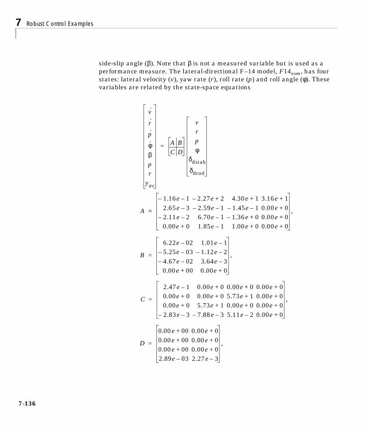
7 Robust Control Examples
7-1
side-slip angle (β). Note that β is not a measured variable but is used as aperformance measure. The lateral-directional F–14 model, F14nom, has fourstates: lateral velocity (v), yaw rate (r), roll rate (p) and roll angle (φ). Thesevariables are related by the state-space equations
v·
r·
p·
φ·
βpr
yac
A BC D
vrpφ
δdstab
δdrud
=
A
1.16e– 1– 2.27e– 2+ 4.30e 1+ 3.16e 1+
2.65e 3– 2.59e– 1– 1.45e– 1– 0.00e 0+
2.11e– 2– 6.70e 1– 1.36e– 0+ 0.00e 0+
0.00e 0+ 1.85e 1– 1.00e 0+ 0.00e 0+
,=
B
6.22e 02– 1.01e 1–
5.25e– 03– 1.12e– 2–
4.67e– 02– 3.64e 3–
0.00e 00+ 0.00e 0+
,=
C
2.47e 1– 0.00e 0+ 0.00e 0+ 0.00e 0+
0.00e 0+ 0.00e 0+ 5.73e 1+ 0.00e 0+
0.00e 0+ 5.73e 1+ 0.00e 0+ 0.00e 0+
2.83e– 3– 7.88e– 3– 5.11e 2– 0.00e 0+
,=
D
0.00e 00+ 0.00e 0+
0.00e 00+ 0.00e 0+
0.00e 00+ 0.00e 0+
2.89e 03– 2.27e 3–
,=
36

F–14 Lateral-directional Control Design
Typing
load F14_nom;
will load the nominal, F–14 plant model into the workspace. The dashed box inFigure 7-67 represents the true airplane, which corresponds to a set of F–14plant models defined by G. Inside the box is the nominal model of the airplanedynamics, F14nom, models of the actuators, AS and AR, and two elements, Winand ∆G, which parameterize the uncertainty in the model. This type ofuncertainty is called multiplicative plant input uncertainty. The transferfunction Win is assumed known, and reflects the amount of uncertainty in themodel. The transfer function ∆G is assumed to be stable and unknown, exceptfor the norm condition, ||∆G||∞ ≤ 1. The aircraft uncertainty is modeled as acomplex full-block, multiplicative uncertainty at the input of the rigid bodyaircraft nominal model. This is the same type of uncertainty description thatwas used in the previous section entitled “HIMAT Robust Performance DesignExample”.
The stabilizer and rudder actuators, AS and AR, are modeled as first ordertransfer functions, . The actuator outputs are their respective rates anddeflections.
A_S = pck(–25,25,[–25;1],[25;0]);A_R = pck(–25,25,[–25;1],[25;0]);
Given the actuator and aircraft nominal models (denoted by Gnom(s)) we alsospecify a stable, 2 × 2 transfer function matrix Win(s), called the uncertaintyweight. These transfer matrices parameterize an entire set of plants, G, whichmust be suitably controlled by the robust controller K.
G := Gnom(I + ∆GWin) : ∆G stable, ||∆G||∞ ≤ 1.
All of the uncertainty in modeling the airplane is captured in the normalized,unknown transfer function ∆G. The unknown transfer function ∆G(s) is used toparameterize the potential differences between the nominal model, Gnom(s),and the actual behavior of the real airplane, denoted by G.
In this example, the uncertainty weight Win is of the form
25s 25+---------------
Win s( ) :=w1 s( ) 0
0 w2 s( )
7-137

7 Robust Control Examples
7-1
for particular scalar valued functions w1(s) and w2(s). The w1(s) weightassociated with the differential stabilizer input is selected to be
. The w2(s) weight associated with the differential rudder input
is selected to be .
w_1 = nd2sys([1 4],[1 160],2);w_2 = nd2sys([1 20],[1 200],1.5);W_in = daug(w_1,w_2);
Hence the set of plants that are represented by this uncertainty weight
with ∆G(s) stable and ||∆G||∞ ≤ 1. Note that the weighting functions are used tonormalize the size of the unknown perturbation ∆G. At any frequency ω, thevalue of |w1(jω)| and |w2(jω)| can be interpreted as the percentage ofuncertainty in the model at that frequency. The dependence on frequency of theuncertainty weight indicates that the level of uncertainty in the airplane'sbehavior depends on frequency. Frequency response plots of weights w1 and w2are shown in Figure 7-69.
om = logspace(–1,3,120);W_ing=frsp(W_in,om);vplot('liv,lm',sel(W_ing,1,1),'-',sel(W_ing,2,2),'--')xlabel('Frequency (rad/sec)')ylabel('Magnitude')
w1 s( ) 2 s 4+( )s 160+---------------------=
w1 s( ) 1.5 s 20+( )s 200+
-----------------------------=
G := F14nom
25s 25+--------------- 0
0 25s 25+---------------
I2
2 s 4+( )s 100+--------------------- 0
0 1.5 s 20+( )s 200+
-----------------------------
∆G s( )+
38
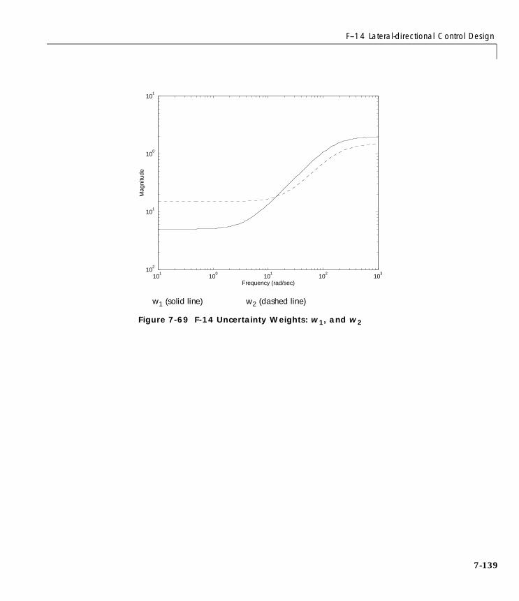
F–14 Lateral-directional Control Design
Figure 7-69 F-14 Uncertainty Weights: w1, and w2
101
100
101
102
103
102
101
100
101
Frequency (rad/sec)
Mag
nitu
de
w1 (solid line) w2 (dashed line)
7-139
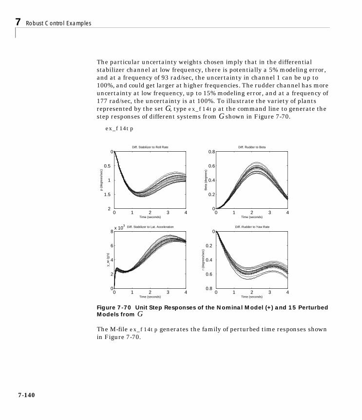
7 Robust Control Examples
7-1
The particular uncertainty weights chosen imply that in the differentialstabilizer channel at low frequency, there is potentially a 5% modeling error,and at a frequency of 93 rad/sec, the uncertainty in channel 1 can be up to100%, and could get larger at higher frequencies. The rudder channel has moreuncertainty at low frequency, up to 15% modeling error, and at a frequency of177 rad/sec, the uncertainty is at 100%. To illustrate the variety of plantsrepresented by the set G, type ex_f14tp at the command line to generate thestep responses of different systems from G shown in Figure 7-70.
ex_f14tp
Figure 7-70 Unit Step Responses of the Nominal Model (+) and 15 Perturbed Models from G
The M-file ex_f14tp generates the family of perturbed time responses shownin Figure 7-70.
0 1 2 3 42
1.5
1
0.5
0Diff. Stabilizer to Roll Rate
Time (seconds)
p (d
egre
es/s
ec)
0 1 2 3 40
0.2
0.4
0.6
0.8Diff. Rudder to Beta
Time (seconds)
Bet
a (d
egre
es)
0 1 2 3 40
2
4
6
8x 10
3 Diff. Stabilizer to Lat. Acceleration
Time (seconds)
y_ac
(g’
s)
0 1 2 3 40.8
0.6
0.4
0.2
0Diff. Rudder to Yaw Rate
Time (seconds)
r (d
egre
es/s
ec)
40

F–14 Lateral-directional Control Design
file: ex_f14tp.mGnom = mmult(F14_nom,daug(sel(A_S,2,1),sel(A_R,2,1)));u = step_tr(0,1,.02,2);ydstab = trsp(Gnom,abv(u,0),4,.05);ydrud = trsp(Gnom,abv(0,u),4,.05);
for i=1:15delta = randn(2,2);delta = delta/norm(delta);p = mmult(Gnom,madd(eye(2),mmult(W_in,delta)));y1 = trsp(p,abv(u,0),4,.05);y2 = trsp(p,abv(0,u),4,.05);ydstab = sbs(ydstab,y1);ydrud = sbs(ydrud,y2);
endcold = ynum(ydrud);index = 2:cold;subplot(221)
vplot(sel(ydstab,2,1),'+',sel(ydstab,2,[index]))title('Diff. Stabilizer to Roll Rate')xlabel('Time (seconds)'), ylabel('p (degrees/sec)')
subplot(222)vplot(sel(ydrud,1,1),'+',sel(ydrud,1,[index]))title('Diff. Rudder to Beta')xlabel('Time (seconds)'), ylabel('Beta (degrees)')
subplot(223)vplot(sel(ydstab,4,1),'+',sel(ydstab,4,[index]))title('Diff. Stabilizer to Lat. Acceleration')xlabel('Time (seconds)'), ylabel('ac_y (g''s)')
subplot(224)vplot(sel(ydrud,3,1),'+',sel(ydrud,3,[index]))title('Diff. Rudder to Yaw Rate')xlabel('Time (seconds)'), ylabel('r (degrees/sec)')
The control design objective is to design a stabilizing controller K such that, forall stable perturbations ∆G(s), with ||∆G||∞ ≤ 1, the perturbed closed-loop systemremains stable, and the perturbed weighted performance transfer function hasan H∞ norm less than 1 for all such perturbations. These mathematicalobjectives exactly fit in the structured singular value framework.
7-141

7 Robust Control Examples
7-1
Controller DesignThe control design block diagram shown in Figure 7-67 is redrawn as F14ICshown in Figure 7-71. F14IC is the 25-state, six-input, six-output open-looptransfer matrix used for control design. The M-file ex_f14ic contains the sysiccommands to generate the F14IC interconnection structure. The M-fileex_f14wt, called from ex_f14ic, creates the weighting functions (Wact, Win, Wn,Wp, and Wβ), the handling qualities models (hqmod_beta, hqmod_p),anti-aliasing filters (anti_filt), the actuator models (AS and AR) and loads thenominal F–14 plant model.
ex_f14ic
file: ex_f14ic.mex_f14wtsystemnames = 'W_in A_S A_R antia_filt hqmod_p hqmod_beta';systemnames = [systemnames 'F14_nom W_act W_n W_P W_beta'];inputvar = '[in_unc2; sn_nois3; roll_cmd; beta_cmd; ';inputvar = [inputvar ' delta_dstab; delta_rud]' ];outputvar = '[ W_in; W_P; W_beta; W_act; roll_cmd; ';outputvar = [outputvar 'beta_cmd; antia_filt + W_n ]' ];input_to_W_in = '[ delta_dstab; delta_rud ]';input_to_A_S = '[ delta_dstab + in_unc(1) ]';input_to_A_R = '[ delta_rud + in_unc(2) ]';input_to_W_act = '[ A_S; A_R ]';input_to_F14_nom = '[ A_S(1); A_R(1) ]';input_to_antia_filt = '[ F14_nom(4) F14_nom(3) F14_nom(2)]';input_to_hqmod_beta = '[ beta_cmd ]';input_to_hqmod_p = '[ roll_cmd ]';input_to_W_beta = '[ hqmod_beta - F14_nom(1) ]';input_to_W_P = '[ hqmod_p - F14_nom(3) ]';input_to_W_n = '[ sn_nois ]';sysoutname = 'F14IC';cleanupsysic = 'yes';sysic
42
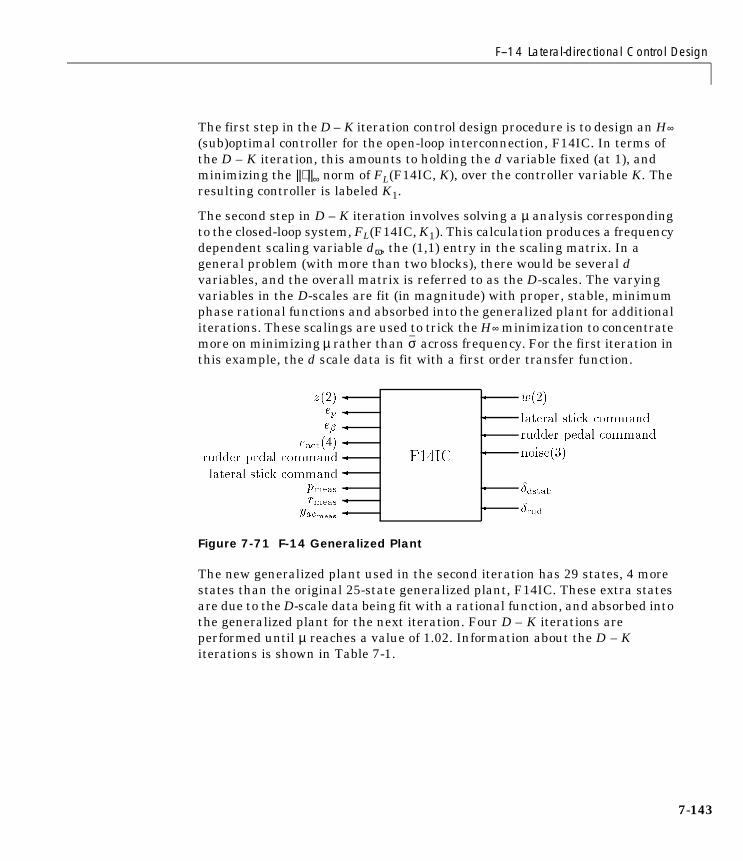
F–14 Lateral-directional Control Design
The first step in the D – K iteration control design procedure is to design an H∞
(sub)optimal controller for the open-loop interconnection, F14IC. In terms ofthe D – K iteration, this amounts to holding the d variable fixed (at 1), andminimizing the ||⋅ ||∞ norm of FL(F14IC, K), over the controller variable K. Theresulting controller is labeled K1.
The second step in D – K iteration involves solving a µ analysis correspondingto the closed-loop system, FL(F14IC, K1). This calculation produces a frequencydependent scaling variable dω, the (1,1) entry in the scaling matrix. In ageneral problem (with more than two blocks), there would be several dvariables, and the overall matrix is referred to as the D-scales. The varyingvariables in the D-scales are fit (in magnitude) with proper, stable, minimumphase rational functions and absorbed into the generalized plant for additionaliterations. These scalings are used to trick the H∞ minimization to concentratemore on minimizing µ rather than across frequency. For the first iteration inthis example, the d scale data is fit with a first order transfer function.
Figure 7-71 F-14 Generalized Plant
The new generalized plant used in the second iteration has 29 states, 4 morestates than the original 25-state generalized plant, F14IC. These extra statesare due to the D-scale data being fit with a rational function, and absorbed intothe generalized plant for the next iteration. Four D – K iterations areperformed until µ reaches a value of 1.02. Information about the D – Kiterations is shown in Table 7-1.
σ
7-143

7 Robust Control Examples
7-1
Table 7-1 F-14 D – K Iteration Information
To replicate these results using D – K iteration, start up dkitgui and press theSETUP button in the main window. The data required in the DK IterationSetup window should be filled in to duplicate the Setup window shown inFigure 7-72. The message “Mu-Synthesis Problem Specification Complete...” will appear in the message bar upon correctly entering therequired data. Return to the main dkitgui window and press the ControlDesign button. This will synthesize controller K1. To run 4 automated D – Kiterations, pull down the Iteration menu and select the number 4 from theAuto Iterate menu.
Iteration Number 1 2 3 4
Total D-Scale Order 0 4 4 4
Controller Order 25 29 29 29
H∞ Norm Achieved 1.562 1.079 1.025 1.017
Peak µ Value 1.443 1.079 1.025 1.017
44

F–14 Lateral-directional Control Design
Figure 7-72 dkitgui F-14 D – K Iteration Setup Window
Analysis of the ControllersThe robust performance properties of the controllers can be analyzed usingµ-analysis methods. Recall that robust performance is achieved if and only iffor every frequency, µ∆(FL(F14IC,K)(jω)) is less than 1. Plots of robustperformance µ of the closed-loop system with K1 and K4 implemented areshown in Figure 7-73. The M-file ex_f14mu generates Figure 7-73 given that
7-145
7 Robust Control Examples
7-1
the original generalized plant, F14IC, and the controller SYSTEM matrices, K1and K4, are in your MATLAB workspace.
ex_f14mu
file: ex_f14mu.m om = logspace(–2,2,60);clp1 = starp(F14IC,K1);clp4 = starp(F14IC,K4);clp1g = frsp(clp1,om);clp4g = frsp(clp4,om);deltaset = [2 2; 5 6];mubnds1 = mu(clp1g,deltaset);mubnds4 = mu(clp4g,deltaset);vplot('liv,lm',mubnds1,'-',mubnds4,'--')xlabel('Frequency (rad/sec)')
The controlled system with K1 implemented does not achieve robustperformance. This conclusion follows from the µ plot, which peaks to a value of1.44, at a frequency of 7 rad/sec. Since µ is 1.44, there is a perturbation matrix
∆G, such that ||∆G||∞ = , and the perturbed weighted performance transfer
functions gets large. After four D – K iterations the peak robust performance µvalue is reduced to 1.02 (Figure 7-73), thereby nearly achieving all of our robustperformance objectives.
To illustrate the robustness of the closed-loop system in the time-domain, timeresponses of the ideal model, the nominal closed-loop system and theworst-case closed-loop system from G (using perturbations of size 1) are shownin Figure 7-74. Controller K4 is implemented in the closed-loop simulations. A1-inch lateral stick command is given at nine seconds, held at 1-inch till 12seconds, and then returns to zero. The rudder is commanded at one second witha positive 1-inch pedal deflection and held at 1-inch till four seconds. At fourseconds a –1-inch pedal deflection is commanded and held to seven seconds andthen returned to zero. One can see from the time responses that the closed-loopresponse is nearly identical for the nominal closed-loop system and theworst-case closed-loop system.
11.44-----------
46

F–14 Lateral-directional Control Design
Figure 7-73 F-14 Robust Performance µ Plots with K1 and K4 Implemented
102
101
100
101
102
0.2
0.4
0.6
0.8
1
1.2
1.4
1.6
Frequency (rad/sec)
mu
mu after 1 iteration (solid) and mu after 4 iterations (dashed)
7-147
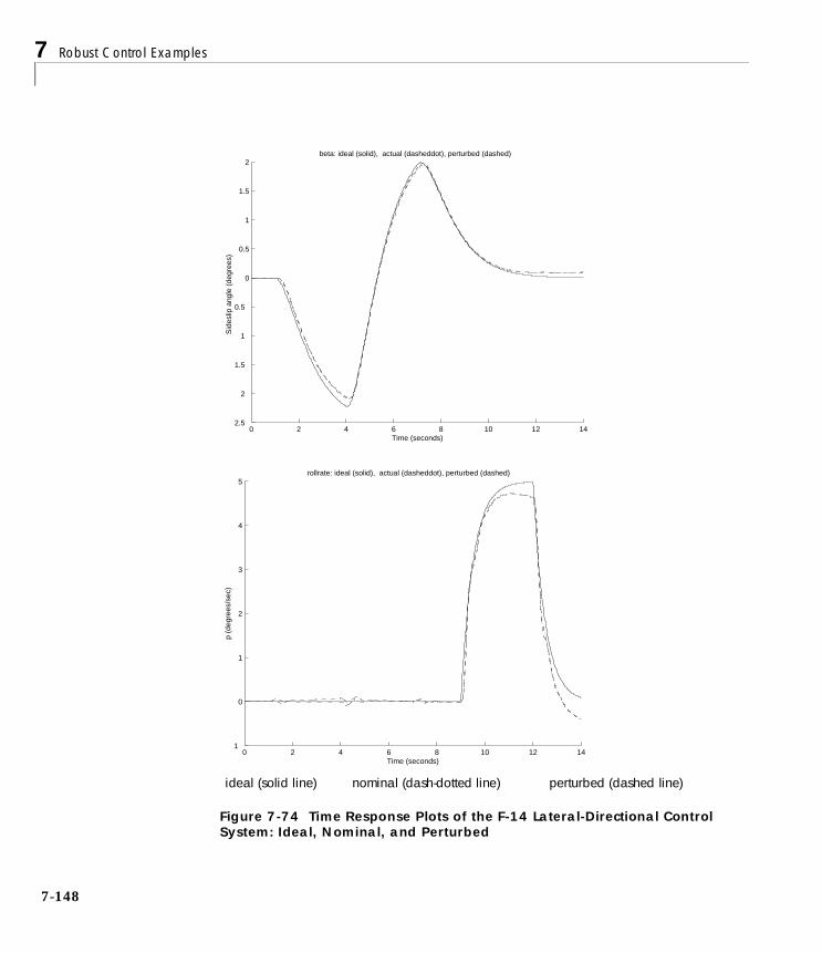
7 Robust Control Examples
7-1
Figure 7-74 Time Response Plots of the F-14 Lateral-Directional Control System: Ideal, Nominal, and Perturbed
0 2 4 6 8 10 12 142.5
2
1.5
1
0.5
0
0.5
1
1.5
2beta: ideal (solid), actual (dasheddot), perturbed (dashed)
Time (seconds)
Sid
eslip
ang
le (
degr
ees)
0 2 4 6 8 10 12 141
0
1
2
3
4
5rollrate: ideal (solid), actual (dasheddot), perturbed (dashed)
Time (seconds)
p (d
egre
es/s
ec)
ideal (solid line) perturbed (dashed line)nominal (dash-dotted line)
48

F–14 Lateral-directional Control Design
The M-file ex_f14s1 contains the sysic commands to generate the F14ICsimulation interconnection structure. ex_f14s2 contains the commands tocalculate the worst-case perturbation of size 1 for K4, the closed-loop timeresponse of the nominal and perturbed systems, and plots the results.
ex_f14s1ex_f14s2
Figure 7-74 validates the frequency domain results showing that the controllersynthesized via D – K iteration, K4, is insensitive to changes in the model. Youwill notice that the roll-rate response of the F–14 tracks the roll-rate commandwell initially and then departs from the command. This is due to a right-halfplane zero in the aircraft model at 0.024 rad/sec.
file: ex_f14s1.msystemnames = 'Win A_S A_R F14_nom antia_filt hqmod_p ';systemnames = [systemnames ' hqmod_beta '];inputvar = '[in_unc2; roll_cmd; beta_cmd; ';inputvar = [inputvar ' delta_dstab; delta_rud]' ];outputvar = '[ W_in; hqmod_p; F14_nom(2); hqmod_beta; 'outputvar = [outputvar ' F14_nom(1); roll_cmd; beta_cmd; '];outputvar = [outputvar 'antia_filt ]' ];input_to_W_in = '[ delta_dstab ; delta_rud ]';input_to_A_S = '[ delta_dstab + in_unc(1) ]';input_to_A_R = '[ delta_rud + in_unc(2) ]';input_to_F14_nom = '[ AS(1); AR(1) ]';input_to_antia_filt = '[F14_nom(4); F14_nom(3); F14_nom(2)]';input_to_hqmod_beta = '[ beta_cmd ]';input_to_hqmod_p = '[ roll_cmd ]';sysoutname = 'F14SIM';cleanupsysic = 'yes';sysic
7-149

7 Robust Control Examples
7-1
file: ex_f14s2.mom = logspace(–2,2,40);delta = wcperf(frsp(clp4,om),deltaset,1,1);sclp4_nom = starp(zeros(2,2),starp(F14SIM,K4));sclp4_pert = starp(delta,starp(F14SIM,K4));ustk = step_tr([0 1 4],[0 1 0],.02,10);upedal = step_tr([0 1 4 7 ],[0 1 –1 0],.02,10);input = abv(ustk,upedal);y4nom = trsp(sclp4_nom,input,14,0.02);y4pert = trsp(sclp4_pert,input,14,0.02);subplot(211), vplot(sel(y4nom,3,1),'-',sel(y4nom,4,1),...
'-.',sel(y4pert,4,1),'--')xlabel('Time (seconds)')ylabel('Side-slip angle (degrees)')title('beta: ideal (solid), actual (dashed-dot),... perturbed (dashed)')
subplot(212), vplot(sel(y4nom,1,1),'-',sel(y4nom,2,1),...'-.',sel(y4pert,2,1),'--')
xlabel('Time (seconds)')ylabel('Roll rate (degrees/sec)')title('roll-rate: ideal (solid), actual (dashed-dot),...perturbed (dashed)')
50

A Process Control Example: Two Tank System
A Process Control Example: Two Tank SystemIn this example we provide a relatively complete description of the entiremodeling, identification, and design process. The experiment is a simple twotank system at Caltech. Other experimental work relating to this system isdescribed by Smith et al. [SmDMS, SmD1, SmD2].
Experimental DescriptionThe system consists of two water tanks in cascade and is shown schematicallyin Figure 7-75. The upper tank (tank 1) is fed by hot and cold water viacomputer controllable valves. The lower tank (tank 2) is fed by water from anexit at the bottom of tank 1. A constant level is maintained in tank 2 by meansof an overflow. A cold water bias stream also feeds tank 2 and enables the tanksto have different steady-state temperatures.
Tank 1 is 5 inches in diameter and 30 inches in height. Tank 2 is 7 inchesin diameter and the overflow maintains the water level at 7 inches. Thisconfiguration maintains the water level in tank 2 at 4 inches below the baseof tank 1. Flow control is obtained via linear electropneumatic actuators witha CV of 1.0. One hundred inches of -inch piping runs from each valve to thetop of tank 1. Approximately 36 inches of pipe connects the tanks, from the baseof tank 1 to the base of tank 2. The tank 2 cold water bias stream is manuallyadjustable between 0.015 and 0.3 gpm. Thermocouples are mounted inchabove the base of each tank. A pressure sensor (0 to 5 psig) provides ameasurement of the water level in tank 1.
All measured signals are filtered with fourth order Butterworth filters, eachwith a cutoff frequency of 2.25 Hz. Twelve bit resolution is used for the A/D andD/A conversions. In digital implementations of the controllers a sample periodof 0.1 seconds has been used.
38---
12---
14---
34---
12---
14---
7-151

7 Robust Control Examples
7-1
Figure 7-75 Schematic Diagram of the Two Tank System
An Idealized Nonlinear ModelThe Two tank example, nonlinear model system is first considered without theactuators or sensors and an ideal nonlinear model is derived. Suitable units areadded to give a basis for the subsequent discussion of the experimental data.The model of the actuators and sensors (including noise) is based onexperimental data and is included later.
Actuator
Actuator
fh command
hot(th) supply
cold (tc) supply
supply at temp td
fc command
fl+fd
h2
fl+fd
fd
fl
Tank2
Tank1
52

A Process Control Example: Two Tank System
We make the following unrealistic assumptions:
• No thermal losses in the system.
• Perfect mixing occurs in both tanks.
• The flow out of tank 1 is related only to the height of tank 1.
• There are no thermal or flow delays.
The system variables are given the following designations.
Tank 1 is considered first. Conservation of mass gives,
Variable Physical quantity
ƒhc Command to hot flow actuator
ƒh Hot water flow into tank 1
ƒcc Command to cold flow actuator
ƒc Cold water flow into tank 1
ƒ1 Total flow out of tank 1
A1 Cross-sectional area of tank 1
h1 Tank 1 water level
t1 Temperature of tank 1
t2 Temperature of tank 2
A2 Cross-sectional area of tank 2
h2 Tank 2 water level
ƒb Flow rate of tank 2 bias stream
tb Temperature of tank 2 bias stream
th Hot water supply temperature
tc Cold water supply temperature
7-153
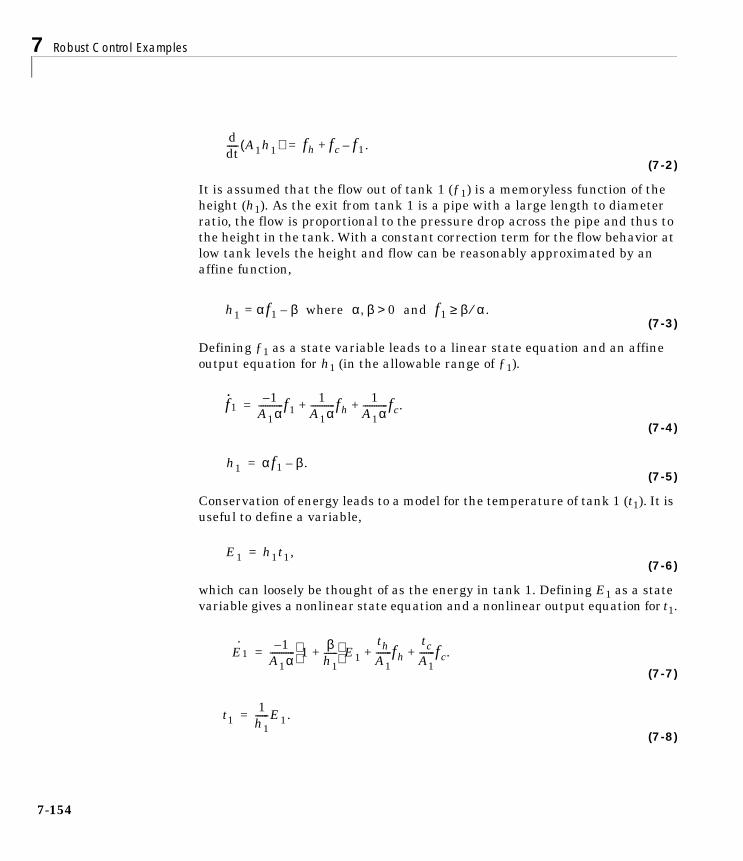
7 Robust Control Examples
7-1
(7-2)
It is assumed that the flow out of tank 1 (ƒ1) is a memoryless function of theheight (h1). As the exit from tank 1 is a pipe with a large length to diameterratio, the flow is proportional to the pressure drop across the pipe and thus tothe height in the tank. With a constant correction term for the flow behavior atlow tank levels the height and flow can be reasonably approximated by anaffine function,
(7-3)
Defining ƒ1 as a state variable leads to a linear state equation and an affineoutput equation for h1 (in the allowable range of ƒ1).
(7-4)
(7-5)
Conservation of energy leads to a model for the temperature of tank 1 (t1). It isuseful to define a variable,
(7-6)
which can loosely be thought of as the energy in tank 1. Defining E1 as a statevariable gives a nonlinear state equation and a nonlinear output equation for t1.
(7-7)
(7-8)
ddt----- A1h1( ) fh fc f1.–+=
h1 α= f1 β– where α β, 0> and f1 β α⁄≥ .
f·11–
A1α-----------f1
1A1α-----------fh
1A1α-----------fc.+ +=
h1 αf1 β .–=
E1 h1t1,=
E·
11–
A1α----------- 1 β
h1------+
E1thA1-------fh
tcA1-------fc.+ +=
t11
h1------E1.=
54

A Process Control Example: Two Tank System
Note that for a fixed h1 the above equations are linear. This will aid in theidentification.
In tank 2 the height (h2) is fixed and the input flow from tank 1 (ƒ1) is oftemperature t1. This gives only one equation:
(7-9)
We will develop a model which has t1 and h1 as inputs and t2 as an output. Thiswill allow us to concatenate the tank 1 and tank 2 models to give a model forthe full system. A more physically motivated model might have t1 and ƒ1 asinputs. The linearizations will differ only by the factor α, so the difference isnot significant.
We can rearrange (7-9) to give,
(7-10)
The output equation for tank 2 is trivial.
Equations (7-4), (7-5), (7-7), (7-8), and (7-10) provide a simple nonlinear modelfor the two tanks. To complete the description of the system a model must beobtained for the actuators and sensors. The uncertainty associated withelements of the model must also be identified. First, we define a suitable set ofunits for our model.
ddt----- A2h2t2( ) f1t1 fbtb f1 fb+( )t2.–+=
t·2h1 β αfb+ +
αA2h2-------------------------------
– t2
h1 β+
αA2h2------------------
t1
fbtbA2h2--------------+ +=
7-155

7 Robust Control Examples
7-1
Normalization UnitsTo quantify the model we define a system of normalized units as follows.
The first two definitions are sufficient to define all of the other units in theproblem. The input flows range from 0 to 2.0 gallons/minute and it isconvenient to define a flow unit at the input by 2.0 gpm = 1.0 funit. Using theabove units the system dimensions are now,
The variable ƒs is a flow scaling factor which converts the input (0 to 1 funits)to flow in hunits3/second. This is used in the tankdemo script.
Physical Variable
Unit Name
0 Unit Definition
1 Unit Definition
temperature tunit tc = 1.0 tunit th = 0.0 tunit
height hunit tank 1 empty tank 1 full
flow funit zero input flow maximum (2.0 gpm)input flow
Variable Value Units
A1 0.0256 hunits2
A2 0.0477 hunits2
h2 0.241 hunits
ƒb 7.4 × 10⁻⁵ hunits3/sec
tb 0.0 tunits
ƒs 0.00028 hunits3/sec/funit
56

A Process Control Example: Two Tank System
Operating RangeThe physical system imposes constraints on the operating region. The mostobvious of these is that as the bias stream is cold, the temperature of tank 2 (t2)must be less than that of tank 1 (t1). Saturation in the actuators prevents tank1 from being completely full of either hot or cold water. The relationshipbetween ƒ1 and h1 can only be modeled by (7-3) for h1 in the range:
The numerical model given below applies only to this range.
In the linear design example the operating range of tank 1 is further reducedto:
Both sets of constraints severely limit the operating regions.
Actuator ModelThere are significant dynamics and saturations associated with the actuatorsand a model of these is included. In the frequency range of interest theactuators can be modeled as a single pole system with rate and magnitudesaturations. The rate saturation has been estimated from observing the effectof triangle waves of different frequencies and magnitudes. The following modelwill be used for the actuators.
(7-11)
with a magnitude limit of 1.0 funits and a rate limit of 3.5 funits/sec. It is therate limit, rather than the pole location, that limits the actuator performancefor most signals. For a linear model some of the effects of rate limiting can beincluded in a perturbation model.
0.15 h1 0.75.≤ ≤
0.25 h1 0.75.≤ ≤
0.25 t1 0.75.≤ ≤
fh1
1 0.05s+( )----------------------------- fhc=
7-157
7 Robust Control Examples
7-1
Experimental Assessment of the ModelWhere possible, the system has been broken into subsystems, which can beidentified independently. For example, the actuators are consideredindependently and tank 1 is identified separately from tank 2. This approachis not necessarily general.
Open-loop ExperimentsStatic measurements of h1 and ƒ1 can be used to obtain estimates of α and βfrom the theoretical relationship: h1 = αƒ1 – β. Note that α appears as a gain inthe nominal model and can also be easily estimated by dynamic measurements.Using such experiments gives the estimates, α = 4876 and β = 0.59.
Open loop experiments have been conducted to test the applicability of themodel and obtain some feel for the level of uncertainty that will be appropriate.Band limited white noise, in several frequency bands, was used for the inputsignals. Data records were 8192 samples in length with sample rates of 1.0 Hzand 10.0 Hz. The transfer function estimates, presented below, have beenobtained by the Welch method, using Hanning windows on sections of the data.The data plotted in the figures comes from several window lengths, typically1024 and 4096. Only the points with good coherency are plotted.
Figure 7-76 shows the estimated transfer function between ƒhc + ƒcc and h1, andthe transfer function predicted from the model (equations (7-4) and (7-5)),including the nominal actuator and Butterworth filter. The experimental datacomes from five experiments at three different levels. For frequencies greaterthan 0.2 Hz, the plotted data comes from an experiment at h1 = 0.47.
Note that the theoretical model is a very close match to the experimental dataover a wide range of frequencies. This suggests that a small perturbationweight is suitable for modeling the discrepancies between the nominal modeland physical system behavior. Note also that the h1 model is independent ofboth h1 and t1. In other words it applies to the entire range of operating points.
For h1 fixed, the E1 state variable equation (7-7) and the t1 output equation(7-8) are linear. Experiments have been performed at h1 = 0.15, 0.25, 0.47,and 0.75. The input waveforms were generated such that ƒhc = –ƒcc whichmaintains a constant h1. Figure 7-77 shows the transfer function between ƒhc– ƒcc(= 2ƒhc) and t1 calculated from the experimental data and estimated fromthe model (equations (7-7) and (7-8). For the data shown h1 = 0.15 and h1 =0.75. The other cases lie between the two curves shown.
58

A Process Control Example: Two Tank System
Figure 7-76 Transfer Function Between ƒhc + ƒcc and h1. Experimental Data and Theoretical Model
10-5
10-4
10-3
10-2
10-1
100
101
10-4 10-3 10-2 10-1 100 10110-5
10-4
10-3
10-2
10-1
100
101
10-4 10-3 10-2 10-1 100 101
frequency: Hz
mag
nitu
de
-600
-500
-400
-300
-200
-100
0
10-4 10-3 10-2 10-1 100 101-600
-500
-400
-300
-200
-100
0
10-4 10-3 10-2 10-1 100 101
frequency: Hz
phas
e -
degr
ees
experimental dataand theoretical
solid line)model (
7-159

7 Robust Control Examples
7-1
Figure 7-77 Transfer Function Between ƒhc – ƒcc and t1. Experimental Data and Models. h1 = 0.15 and h1 = 0.75.
10-4
10-3
10-2
10-1
100
101
10-4 10-3 10-2 10-1 100 10110-4
10-3
10-2
10-1
100
101
10-4 10-3 10-2 10-1 100 101
frequency: Hz
mag
nitu
de
h1 = 0.15
h1 = 0.75
-450
-400
-350
-300
-250
-200
-150
-100
-50
0
10-4 10-3 10-2 10-1 100 101-450
-400
-350
-300
-250
-200
-150
-100
-50
0
10-4 10-3 10-2 10-1 100 101
frequency: Hz
phas
e -
degr
ees
h1 = 0.15
h1 = 0.75
experimental dataand models (solid lines)
60

A Process Control Example: Two Tank System
The nominal model/physical system discrepancies are far more significant forthe t1 case. A larger t1 perturbation weight is required to cover thesediscrepancies. A more complete discussion on this issue is given in the“Perturbation Model” section.
Similar analyses have been performed on tank 2. The open loop data is lessconclusive due to observing the system through tank 1 and a higher noise level.The available data does confirm the theoretical model but to a lower frequencythan that for tank 1. More definitive results have been obtained for tank 2 withthe closed-loop experiments.
Closed-loop ExperimentsWe will look at a closed-loop method of estimating a suitable uncertainty levelfor the model. This involves using a relay to induce limit cycling and is basedon an auto-tuning method proposed by Åström and Hägglund [AstH]. Moredetail on using such approaches for estimating uncertainty levels is describedby Smith and Doyle [SmD2].
Applying a relay in a feedback loop may drive the closed-loop system into stablelimit cycles. This technique works for a large class of systems including the twotank system. In the experiments performed here a decoupled controller (intoheight and temperature loops) was used with a relay in the temperaturecontrol loop. This allowed stable control of the tank height (h1) and producedlimit cycles in t1. These experiments were performed at fixed heights (h1 = 0.15,0.25, 0.47, and 0.75).
With a simple relay the closed-loop system will limit cycle at the frequencywhere the response has a phase of 180 degrees. The gain at this frequency canalso be estimated from the input/output data. This experiment will identify thesystem at a single point. Using this information, a new controller is designedto introduce some lead into the closed-loop system. This new closed-loop systemhas limit cycles at a higher frequency giving an additional point at which theplant can be identified. In practice this technique can be repeated until thenonlinear and/or inconsistent effects dominate and the closed-loop system nolonger limit cycles consistently. This also provides information on thefrequency at which uncertainty should dominate in the model.
Details of the application of this approach to tank 1 are given in [SmD2]. Toillustrate the concept, the configuration used to induce limit cycles in t1 isshown in Figure 7-78.
7-161

7 Robust Control Examples
7-1
Figure 7-78 Closed-Loop Configuration for Relay Limit Cycle Experiments of t1.
A series of controllers, Ci in Figure 7-78, was applied. These were used tointroduce differing amounts of lead into the closed-loop system, giving differinglimit cycle frequencies and amplitudes. A typical time response for such anexperiment is shown in Figure 7-79. In this manner limit cycles were inducedin the t1 loop. The highest frequency at which a limit cycle could be induced was0.023 Hz. We will subsequently see that this can be used as a heuristic fordetermining an appropriate perturbation weight for t1.
The tank 2 model was similarly studied. Figure 7-80 presents the limit cycledata obtained for tank 2. The E1 to t2 theoretical transfer function (for fixed h1)is shown for h1 = 0.15, 0.25, 0.47, and 0.75. Also shown are the points identifiedfrom each experiment. It was not possible to induce consistent limit cycles atfrequencies above 0.03 Hz, indicating that this is a frequency at which theuncertainty should dominate in the model.
Height, h1, is controlled by the proportional controller, Kh. R denotes the relay andCi denotes one of a series of lead controllers used to adjust the limit cycle frequency.
62

A Process Control Example: Two Tank System
Figure 7-79 Closed-Loop Relay LImit Cycle Experiment Controller: C1
0.3
0.35
0.4
0.45
0.5
0.55
0.6
0 50 100 150 200 250 300 350 400
seconds
leve
l & te
mp
0
0.1
0.2
0.3
0.4
0.5
0.6
0.7
0.8
0.9
1
0 50 100 150 200 250 300 350 400
seconds
hot &
col
d flo
ws
7-163
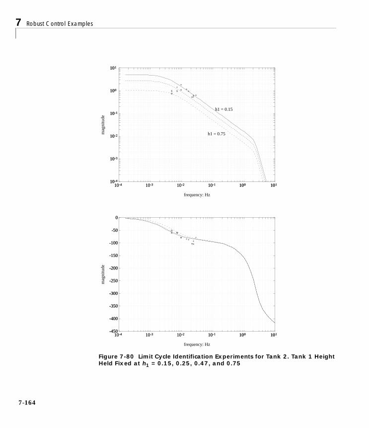
7 Robust Control Examples
7-1
Figure 7-80 Limit Cycle Identification Experiments for Tank 2. Tank 1 Height Held Fixed at h1 = 0.15, 0.25, 0.47, and 0.75
10-4
10-3
10-2
10-1
100
101
10-4 10-3 10-2 10-1 100 101
ox x
+*
++
+
*+*+
10-4
10-3
10-2
10-1
100
101
10-4 10-3 10-2 10-1 100 101
frequency: Hz
mag
nitu
de
h1 = 0.15
h1 = 0.75
-450
-400
-350
-300
-250
-200
-150
-100
-50
0
10-4 10-3 10-2 10-1 100 101
ox x+
*+ ++
*+*
+
-450
-400
-350
-300
-250
-200
-150
-100
-50
0
10-4 10-3 10-2 10-1 100 101
frequency: Hz
mag
nitu
de
64

A Process Control Example: Two Tank System
Developing the Interconnection Model for DesignThe problem considered is the control of t1 and t2 for command response. Thedesired closed-loop configuration is illustrated in Figure 7-81. The controllerhas access to both the reference inputs and the temperature measurements. Itwould be possible (although more restrictive) to design a controller which usedonly the error between the temperature measurements and the setpoints.
Figure 7-81 Closed-Loop Design Problem.
The layout of the interconnection structure is illustrated in Figure 7-82. Thesubsequent sections will develop a perturbed model and the necessary designweights for the design problem.
The t1 and t2 reference signals are denoted by t1cmd and t2cmd, respectively. Noise is assumed to enter within the tank system block.
7-165

7 Robust Control Examples
7-1
Figure 7-82 Interconnection Structure for the Design Problem
Linearized Nominal ModelThe top tank model, given in equations (7-4), (7-5), (7-7), and (7-8), can belinearized to give the following model.
(7-12)
f·1
E·
1
1–αA1----------- 0
β t1
A1h1--------------
β h1+( )–
αA1h1------------------------
f1
E1
=
+
1αA1-----------
1αA1-----------
thαA1-----------
tcαA1-----------
fh
fc
66

A Process Control Example: Two Tank System
(7-13)
The steady state values of h1 and t1 are given by and , respectively.
A linearized model for tank 2 is given by,
(7-14)
As above, denotes the steady state value of t2, and can be calculated by,
where the steady state flow out of tank 1 is,
To complete the linearized nominal model we must select a nominal operatingpoint. The demo script, tankdemo, develops the equations in the form givenabove and uses the values and for the actual design.
Perturbation ModelWe must now select a perturbation model structure for our robust controlmodel. This involves determining the manner in which the perturbations enterthe model, and selecting appropriate frequency dependent weights tonormalize the perturbations. The guiding approach is to make the modelperturbations match our estimate of uncertainty in the physical system asclosely as possible.
For example, it is reasonable to attribute some dynamic uncertainty to theactuators, which suggests that uncertainty at the inputs, ƒh and ƒc, isappropriate. It is also reasonable to consider this uncertainty as being relativewith respect to the input. A potential model may have uncertainty modeled by
h1
t1
α 0
αt1–
h1------------
1
h1------
f1
E1
=
h1 t1
t·2h1 β αfb+ +( )–
αA2h2---------------------------------------- t2
t1 t2+αA2h2------------------
h1 β+αA2h2------------------
h1
t1
+= .
t2
t2f1 t1 fbtb+
f1 fb+---------------------------=
f1 αh1 β–= .
h1 0.75= t1 0.75=
7-167

7 Robust Control Examples
7-1
multiplicative perturbations on ƒh and ƒc. This is particularly appropriate forhigh condition number plants as it prevents the controller from inverting theplant from the input in a robust design.
We already know from the open-loop experiments that there is a significantamount of dynamic uncertainty in the t1 response. This is due primarily tomixing and heat loss. This suggests that a multiplicative perturbation on thet1 output is also an appropriate model.
There are many choices available and we have chosen to capture theuncertainty with multiplicative perturbations on h1, t1, and t2. One could alsoadd perturbations on ƒh and ƒc, although it is doubtful that the additionalmodel complexity (it would now have five perturbations), would be worthwhile.Arguably, we do not have such a detailed model of the uncertainty in this case.
Figure 7-83 illustrates the perturbed linear model of the two tank system. Thethree perturbations, ∆1, ∆2, and ∆3, model the uncertainty in h1, t1, and t2,respectively. Note that they are multiplicative perturbations and that t2 isinfluenced by all three perturbations. The nominal tank 1 model is describedby equations (7-12) and (7-13), and the nominal tank 2 model is given byequation (7-14).
Figure 7-83 Schematic Representation of the Perturbed, Linear, Two Tank Model
68
A Process Control Example: Two Tank System
To complete this model we must specify the perturbation weights, Wh1, Wt1,and Wt2. As we might expect, it is not possible to precisely determine theamount of uncertainty in the system. At best, we look for a rough frequencydependent bound. We discuss some of the ad-hoc means for getting suitableweights below.
• Accuracy limits on actuators and sensors. Equipment manufacturers willoften specify accuracy limits on such equipment and this serves as a usefulstarting point for at least the steady-state uncertainty of some systemcomponents.
Known rate limits can also be viewed as limiting the high frequency behaviorof an actuator. Rate limits are nonlinear and it will not be possible tocompletely capture their effects with even a linear perturbation model.However, these limits may give an approximate estimate of the bandwidthof an actuator.
• Linearization constants. If a nonlinear model is available, then examiningthe variation in the linearization constants across the expected range ofoperation will give an estimate of appropriate levels of uncertainty forelements of the model. For example, we could examine how the time constantof the tank 1 t1 response varied across the h1 operating range.
Again, this is only a crude approximation. The full nonlinear behavior of theplant is not captured by considering a series of frozen linear systems atvarious operating points.
• Open-loop identification experiments. Comparing experimentally estimatedtransfer functions to those predicted by a nominal model gives a goodestimate of the model/system discrepancy at each frequency.
• Closed-loop identification experiments. These are preferred over open-loopidentification experiments for a number of reasons:
Closing the loop automatically biases the plant to the correct operating point.This provides appropriate signals for identification as they are close to thosesignals that will occur in final closed-loop operation;
The achievable performance (at least in terms of closed-loop bandwidth) islimited by the uncertainty at frequencies close to the loop cross-overfrequency. Open-loop experiments tend to emphasize the frequencies wherethe plant gain is high – typically steady-state in many process controlsystems. This is simply due to the significantly larger response on the plant
7-169

7 Robust Control Examples
7-1
at those frequencies. On the other hand, using closed-loop identificationexperiments places the emphasis on the loop cross-over frequencies, which ismore important for the ultimate closed-loop design.
The analysis of closed-loop identification experiments needs to be performedcarefully. The measurement noise is no longer uncorrelated with the inputand output signals and its effect cannot be removed simply by averaging.Van den Hof et al. [VdHSB] give a suitable means of dealing with thissituation.
• Closed-loop relay experiments. The “Closed-loop Experiments” section brieflydiscussed using relays to induce closed-loop limit cycle operation. A largeclass of systems (including the two tank system) will limit cycle under thesecircumstances. The frequency at which the system limit cycles is simply theloop cross-over frequency and we can investigate the achievable closed-loopbandwidth by using lead controllers to make the system limit cycle atsuccessively higher frequencies.
Beyond some frequency the system no longer has a limit cycle; the dynamicsare no longer dominated by linear time-invariant behavior. The heuristic isthat at such frequencies the effect of the perturbations should dominate themodel. This is easy to apply when a multiplicative perturbation is used;when the magnitude of the weight is greater than one, the perturbationdominates the model.
This approach was used for determining the frequencies at which |Wt1| and|Wt2| exceeded one.
• Systematic design, implementation, and evaluation. In other words, try itand see. Clearly, closed-loop implementation of the controller design shouldbe the final arbiter of a suitable model. One approach is to design a series ofcontrollers, each with a smaller perturbation weight (i.e., assuming lessuncertainty), and implement these controllers on the physical system.Setting the weight too high will give a conservative result as performance isunnecessarily traded off against robust stability. A weight that is too smallwill lead to a controller design that exhibits too little robustness, or is evenunstable, in practice. Balas and Doyle [BalDoy1, BalDoy2] give details of asimilar approach to a flexible structure problem.
At first it seems that this approach does not save any effort as we mustdesign and implement all potential controllers. However, it does provideinformation about the appropriate level of uncertainty, and we may be able
70

A Process Control Example: Two Tank System
to conduct simpler experiments (for example designing SISO controllers toevaluate Wh1) to gain information about components within the system. Thisinvolves less effort than attempting to tune all perturbation weights at once.
These issues have been considered in developing the perturbation weights. Themost important aspects of the two tank problem were considered to be:
• The nominal model for h1 is very accurate up to at least 0.3 Hz.
• Limit cycle experiments in the t1 loop suggest that uncertainty shoulddominate above 0.02 Hz.
• There is about 180 degrees of additional phase lag in the t1 model(at h1 = 0.75) at about 0.02 Hz. There is also a significant gain loss at thisfrequency. These effects are the result of the unmodeled mixing dynamics.
• Limit cycle experiments in the t2 loop suggest that uncertainty shoulddominate above 0.03 Hz.
It is not surprising that there is less uncertainty associated with tank 2; mostof the temperature uncertainty arises from the mixing dynamics and tank 2 issomewhat smaller than tank 1. The perturbation weights are illustratedgraphically in Figure 7-84.
7-171
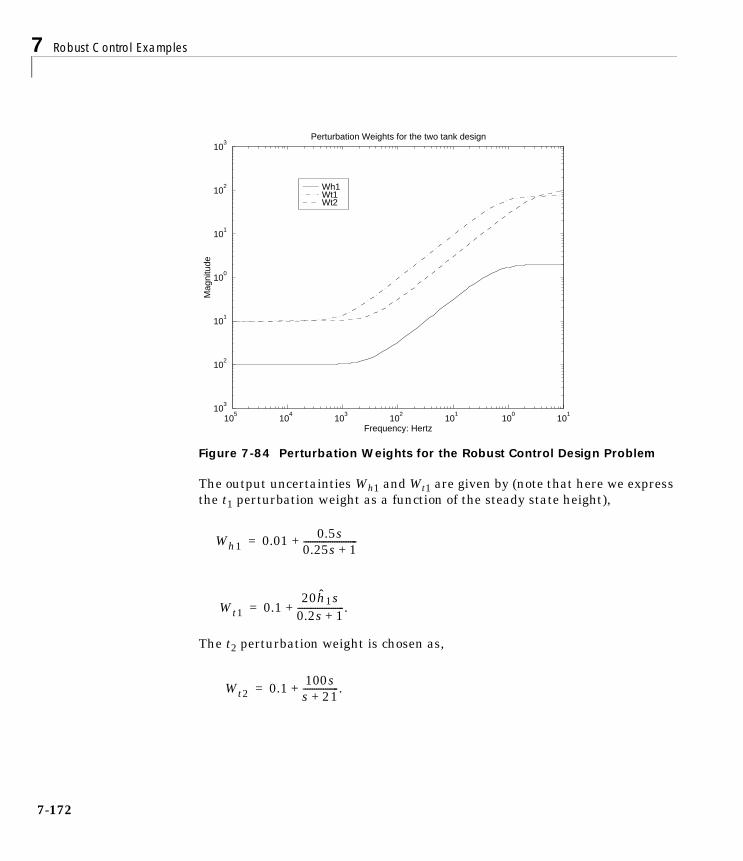
7 Robust Control Examples
7-1
Figure 7-84 Perturbation Weights for the Robust Control Design Problem
The output uncertainties Wh1 and Wt1 are given by (note that here we expressthe t1 perturbation weight as a function of the steady state height),
The t2 perturbation weight is chosen as,
Wh1Wt1Wt2
105
104
103
102
101
100
101
103
102
101
100
101
102
103
Frequency: Hertz
Mag
nitu
de
Perturbation Weights for the two tank design
Wh1 0.01 0.5s0.25s 1+------------------------+=
Wt1 0.120h1s
0.2s 1+---------------------.+=
Wt2 0.1100ss 21+----------------.+=
72

A Process Control Example: Two Tank System
Sensor Noise WeightsThe sensor dynamics are insignificant relative to the dynamics of the rest of thesystem. This will not be true of the sensor noise. The potential sources of noiseinclude electronic noise in thermocouple compensators, amplifiers, and filters,radiated noise from the stirrers, and poor grounding (this is, after all, aninexpensive laboratory experiment).
We will model the noise by adding a weighted unknown input to h1, t1, and t2.Smoothed FFT analysis has been used to estimate the noise on a quiescentsystem. This gives the following weights.
Wh1noise = 0.01
Wt1noise = 0.03
Wt2noise = 0.03
The design considered in tankdemo.m uses measurements of only t1 and t2. Theweight Wh1noise is unnecessary for this case but is included so that you caninvestigate different control configurations.
There are additional disturbances or noises associated with the measurementsthat are not, strictly speaking, sensor noise. For example, in tank 2 theimperfect mixing of the bias stream causes variations in the temperaturemeasurement. The inclusion of such noises here does not affect theperformance requirements of the controller.
Specifying the Design RequirementsIt now remains to include in the interconnection structure (refer to Figure 7-82)the weighting functions that specify performance. These are the referenceweights, error weights, and actuator weights. Arguably, noise weights anddisturbance weights also fall into those categories although we have chosen topresent the noise weights as part of the system model above. In a more generalsetting weighted disturbances or more complex error specifications might alsobe considered.
The weights should be considered as frequency dependent, relative weightings.For example, it is the relative size of the reference weights and noise weightsthat determines the extent to which the final controller design emphasizesreference tracking error over sensor noise rejection.
7-173
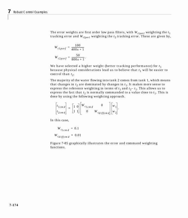
7 Robust Control Examples
7-1
The error weights are first order low pass filters, with Wt1perƒ weighting the t1tracking error and Wt2perƒ weighting the t2 tracking error. These are given by,
We have selected a higher weight (better tracking performance) for t1because physical considerations lead us to believe that t1 will be easier tocontrol than t2.
The majority of the water flowing into tank 2 comes from tank 1, which meansthat changes in t2 are dominated by changes in t1. It makes more sense toexpress the reference weighting in terms of t1 and t2– t1. This allows us toexpress the fact that t2 is normally commanded to a value close to t1. This isdone by using the following weighting approach.
In this case,
Figure 7-85 graphically illustrates the error and command weightingfunctions.
Wt1perf100
400s 1+----------------------=
Wt2perf50
800s 1+---------------------- .=
t1cmd
t2cmd
1 01 1
Wt1cmd0
0 Wtdiffcmd
w1
w2
.=
Wt1cmd0.1=
Wtdiffcmd 0.01=
74

A Process Control Example: Two Tank System
Figure 7-85 Performance Weights for the Robust Control Design Problem
In the case of the actuation weights we would like to weight both the amplitudeand the rate of the actuator. This can be done by weighting ƒhc (and ƒcc) with afunction that rolls up at high frequencies. An alternative approach can be usedwhen we have a first order actuator model.
Using ƒhc as an example; the approach is to create an actuator model with ƒhand dƒh/dt as outputs. These can then be separately weighted with constantweights. Note that this approach has the advantage of reducing the number ofstates in the interconnection structure, and hence in the final design. Figure7-86 illustrates the form of such a weighted actuator model.
Wt1perf
Wt2perf
Wt1cmd
Wtdiffcmd
105
104
103
102
101
100
101
103
102
101
100
101
102
103
Frequency: Hertz
Mag
nitu
de
Perturbation Weights for the two tank design
7-175
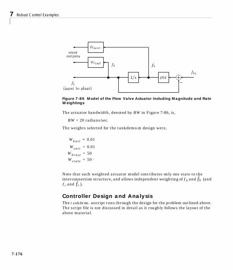
7 Robust Control Examples
7-1
Figure 7-86 Model of the Flow Valve Actuator Including Magnitude and Rate Weightings
The actuator bandwidth, denoted by BW in Figure 7-86, is,
BW = 20 radians/sec.
The weights selected for the tankdemo.m design were,
Note that each weighted actuator model contributes only one state to theinterconnection structure, and allows independent weighting of ƒh and (andƒc and ).
Controller Design and AnalysisThe tankdemo.m script runs through the design for the problem outlined above.The script file is not discussed in detail as it roughly follows the layout of theabove material.
Whact 0.01=
Wcact 0.01=
Whrate 50=
Wcrate 50= .
f·hf·c
76

A Process Control Example: Two Tank System
Design IssuesOne issue regarding the design approach is worth noting. We begin bydesigning for the nominal case. This is done by selecting out of theinterconnection structure the perturbation inputs and outputs (v and z). Thisdesign achieved a closed-loop H∞ norm of γ = 0.9082. This is a lower bound onthe achievable value of µ for robust performance.
The response of the nominal controller (k0 in the script) is simulated, and isshown in Figure 7-87. This is a check on the applicability of our performanceweights. In general, the inclusion of the robustness in the design problem willhave the effect of trading off this nominal performance in order to improve thestability robustness. Simulating the nominal design gives a rough idea of whatthe time domain performance implied by the weights.
7-177
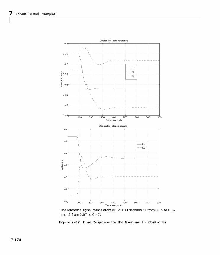
7 Robust Control Examples
7-1
Figure 7-87 Time Response for the Nominal H• Controller
fhcfcc
0 100 200 300 400 500 600 700 8000.2
0.3
0.4
0.5
0.6
0.7
0.8
Time: seconds
Act
uato
rs
Design k0, step response
h1
t1
t2
0 100 200 300 400 500 600 700 8000.45
0.5
0.55
0.6
0.65
0.7
0.75
0.8
Time: seconds
Mea
sure
men
ts
Design k0, step response
The reference signal ramps (from 80 to 100 seconds) t1 from 0.75 to 0.57, and t2 from 0.67 to 0.47.
78

A Process Control Example: Two Tank System
The demo file, tankdemo, uses this interconnection structure for the robustperformance design. In the demo example three D – K iterations are performed.In each of the D-scale fitting calls (performed with the function musynfit),second order D-scale fits were selected. The final value of µ achieved is 1.73.Further iterations may give further improvements; for this example it wasdecided to stop at this point.
Closed-Loop AnalysisWe will run through a typical series of analyses for our design and brieflydiscuss the aspects of interest. The procedure guarantees closed-loop stability(although it is still worth checking to make sure numerical problems have notinvalidated the design) but the controller need not be stable. It often is stableand this is preferable for implementation purposes.
The frequency response of the controller is given in Figure 7-88. We note thatthe controller rolls off around the frequency range where the uncertaintiesstart to become larger. This is what we would expect from a classical point ofview.
Note that there is not a great deal of low frequency gain. We will subsequentlysee that this is because the noise level is high relative to the error weighting.
An identical simulation is run to give an idea of the loss of nominalperformance in the time domain. This is not intended as a comparison betweenk0 and kmu. A more appropriate comparison would also include a simulation ofa perturbed system. The function dypert can be used to select the worst caseperturbation. The nominal response of kmu is shown in Figure 7-89. There islittle deterioration in the nominal response for controller kmu.
7-179

7 Robust Control Examples
7-1
Figure 7-88 Frequency Response of the µ Synthesis Controller
105
104
103
102
101
100
101
105
104
103
102
101
100
101
Frequency: Hertz
Mag
nitu
de
Controller: kmu
105
104
103
102
101
100
101
400
300
200
100
0
100
200
300
Frequency: Hertz
Pha
se (
degr
ees)
Controller: kmu
80

A Process Control Example: Two Tank System
Figure 7-89 Nominal Time Response for the kmu Controller
h1
t1
t2
0 100 200 300 400 500 600 700 8000.45
0.5
0.55
0.6
0.65
0.7
0.75
0.8
Time: seconds
Mea
sure
men
ts
Design kmu, step response
fhcfcc
0 100 200 300 400 500 600 700 8000.2
0.3
0.4
0.5
0.6
0.7
0.8
Time: seconds
Act
uato
rs
Design kmu, step response
The reference signal ramps (from 80 to 100 seconds) t1 from 0.75 to 0.57, and t2 from 0.67 to 0.47
7-181

7 Robust Control Examples
7-1
The tradeoff between robustness and performance can be further studied byindependently calculating µ for robust stability, and the closed-loop nominalperformance. Note that robust stability is a µ test on the v to z block of theclosed-loop transfer function in Figure 7-82. Three 1 × 1 blocks are specified forthe robust stability block structure. The robust performance is given by themaximum singular value of the w to e block of the closed-loop transfer function.Figure 7-90 compares these with robust performance over the frequency range.
Figure 7-90 Robust Performance, Robust Stability, and Nominal Performance for the µ Synthesis Controller
Figure 7-90 illustrates that the nominal performance limits the low frequencyrobust performance. Robust stability does not become an issue except around0.01 Hz. This is not surprising as the perturbation weights begin to increasearound this frequency, yet the controller has only begun to roll off.
These issues can be further investigated by examining smaller subblocks of theD-scaled closed-loop system. This form of analysis has been referred to asM-analysis in the aerospace robust control community, simply because theclosed-loop system was habitually designated by M. It allows us to determinewhich inputs and outputs are limiting the achievable robust performance. This
rob perf
rob stab
nom perf
105
104
103
102
101
100
101
0
0.2
0.4
0.6
0.8
1
1.2
1.4
1.6
1.8
Frequency: Hertz
mu analysis: controller kmu
82

A Process Control Example: Two Tank System
analysis is performed by calculating the µ upper bound, DMD–1, at eachfrequency. We then look at the maximum singular values of the appropriatesubblocks. The example will serve as clarification.
The performance inputs, w, are divided into two group:
• reference commands
• noise
There are three groups of performance outputs:
• tracking errors
• actuator penalties
• actuator rate penalties
This give six 2 × 2 transfer function blocks, and for each of these we calculatethe maximum singular value as a function of frequency.
The results for the temperature inputs are shown in Figure 7-91. Thecalculated nominal performance (maximum singular value of the w to etransfer function) is an upper bound for each of the subblock calculations andserves as a comparison point.
The temperature reference command to tracking error transfer functiondominates those shown in Figure 7-91. However it is only really significant,with respect to the nominal performance, in the frequency range 0.001 to 0.01Hz. It also has some contribution at lower frequencies. By contrast, theactuator penalty has almost no effect on the design. We could change thisweight significantly without affecting the design. The actuator rate penaltystarts to influence the design at frequencies above 0.01 Hz.
Figure 7-92 illustrates the subblocks corresponding to the noise inputs. It isimmediately clear that the noise to tracking error transfer function dominatesthe design at low frequencies. To improve the low frequency nominalperformance (and the low frequency robust performance) we must reduce thenoise weights. In practical terms this means buying higher quality sensors.
7-183

7 Robust Control Examples
7-1
Figure 7-91 DMD–1 Analysis for Temperature Reference Command Inputs
cmds > errorsrob perf nom perf
105
104
103
102
101
100
101
0
1
2DMDinv analysis for kmu: temp cmds > errors
Frequency: Hertz
cmds > actuatorrob perf nom perf
cmds > act raterob perf nom perf
105
104
103
102
101
100
101
0
1
2DMDinv analysis for kmu: temp cmds > act rate
Frequency: Hertz
105
104
103
102
101
100
101
0
1
2DMDinv analysis for kmu: temp cmds > actuator
Frequency: Hertz
*robust performance and nominal performance are included for comparison
84

A Process Control Example: Two Tank System
Figure 7-92 DMD–1 Analysis for Noise Inputs
noise > errorsrob perf nom perf
105
104
103
102
101
100
101
0
1
2DMDinv analysis for kmu: noise > errors
Frequency: Hertz
noise > actuatorrob perf nom perf
noise > act raterob perf nom perf
105
104
103
102
101
100
101
0
1
2DMDinv analysis for kmu: noise > act rate
Frequency: Hertz
105
104
103
102
101
100
101
0
1
2
Frequency: Hertz
DMDinv analysis for kmu: noise > actuator
*robust performance and nominal performance are included for comparison
7-185

7 Robust Control Examples
7-1
A similar analysis can be used to determine which aspects of the design arelimiting robust stability. In this case, there are three transfer functions toexamine; v1 to z1, etc. These are illustrated in Figure 7-93 and compared toboth robust performance and robust stability.
Figure 7-93 DMD–1 Analysis for the Perturbations
As we would expect, the h1 perturbation has little influence on the design.Recall that the uncertainty associated with the h1 output is small compared tothe temperature outputs. We can also see that the t1 perturbation weightdominates the robust stability. This is still not large compared with robust
h1 pert tfrob perf rob stab
105
104
103
102
101
100
101
0
1
2DMDinv analysis for kmu: h1 perturbation
Frequency: Hertz
t1 perf tfrob perf rob stab
105
104
103
102
101
100
101
0
1
2DMDinv analysis for kmu: t1 perturbation
Frequency: Hertz
t2 pert tfrob perf rob stab
105
104
103
102
101
100
101
0
1
2
Frequency: Hertz
DMDinv analysis for kmu: t2 perturbation
*robust performance and nominal performance are included for comparison
86

A Process Control Example: Two Tank System
performance, but if we wish to improve the robust stability, we must reduceWt1. In practical terms this means that we must invest more effort in modelingand identifying some of the tank 1 mixing dynamics.
We can also apply this type of analysis at a single frequency. To do this wewould simply examine the mu upper bound for the closed-loop system at aparticular frequency. A column with large numbers would indicate that thecorresponding input was dominating the design. Similarly, a row of largenumbers would indicate that the corresponding output was dominating thedesign.
This form of analysis is very useful in giving engineering information about thelimiting factors in the design. As we have illustrated above, it can be used toindicate where additional effort (in terms of further modeling/identification, orhigher quality sensing) is required to improve robust performance.
Experimental EvaluationWe present an experimental comparison between a µ synthesis design and amore standard loopshaping controller on the two tank system. The designshown here is not identical to that given above as it was calculated andimplemented several years before µ-Tools was written. However, the methodand relative weightings were similar.
A simple SISO style loopshaping technique has been used to design controllers(Kloop) for comparison purposes. One of the worst case plant conditions, (h1 =0.75, t1 = 0.25), was selected as a nominal design point. The controller simplyinverts the plant to a diagonal loopshape. It is now well known that thistechnique will not work well for high condition number plants, particularlythose with uncertainty at the input. Refer to the work of Skogestad et al.[SkoMD] for further details on this point.
The loopshape chosen was:
Figure 7-94 shows the magnitude of the frequency response of Kloop.
t1 loop 1001 3000s+( )
------------------------------=
t2 loop 1001 5000s+( )
------------------------------=
7-187

7 Robust Control Examples
7-1
Figure 7-94 Magnitude Response of the Loopshaping Controller: Kloop
Both controllers have been tested over a wide range of commands. Figure 7-95shows a typical command tracking response for the Kloop and Figure 7-96 showsthe same response for Kmu. The oscillatory behavior of the loopshapingcontroller cannot be alleviated by selecting loopshapes that have a lowercrossover frequency. These merely produce lower frequency and higheramplitude oscillations. It is the method of inverting the plant that leads to thisproblem.
10-2
10-1
100
101
102
103
10-5 10-4 10-3 10-2 10-1 100 10110-2
10-1
100
101
102
103
10-5 10-4 10-3 10-2 10-1 100 101
frequency: Hz
88

A Process Control Example: Two Tank System
Figure 7-95 Experimental Command Response: Controller Kloop with Input Temperature Ramps Going from t1 = 0.75, t2 = 0.67 at 80 Seconds to t1 = 0.55, t2 = 0.47 at 100 Seconds
0
0.1
0.2
0.3
0.4
0.5
0.6
0.7
0.8
0.9
1
0 100 200 300 400 500 600 700 800
Kloop command response: plant outputs
0
0.1
0.2
0.3
0.4
0.5
0.6
0.7
0.8
0.9
1
0 100 200 300 400 500 600 700 800
time: seconds
h1
t1
t2
0
0.1
0.2
0.3
0.4
0.5
0.6
0.7
0.8
0.9
1
0 100 200 300 400 500 600 700 800
commandfh
fc command
Kloop command response: actuators
time: seconds
7-189
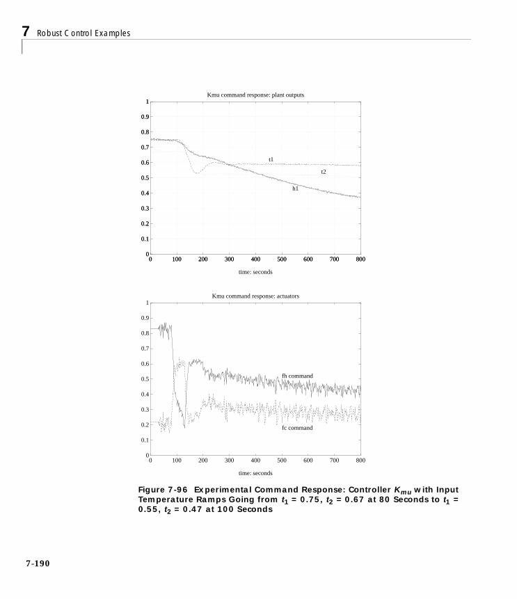
7 Robust Control Examples
7-1
Figure 7-96 Experimental Command Response: Controller Kmu with Input Temperature Ramps Going from t1 = 0.75, t2 = 0.67 at 80 Seconds to t1 = 0.55, t2 = 0.47 at 100 Seconds
0
0.1
0.2
0.3
0.4
0.5
0.6
0.7
0.8
0.9
1
0 100 200 300 400 500 600 700 8000
0.1
0.2
0.3
0.4
0.5
0.6
0.7
0.8
0.9
1
0 100 200 300 400 500 600 700 800
time: seconds
Kmu command response: plant outputs
t1
t2
h1
0
0.1
0.2
0.3
0.4
0.5
0.6
0.7
0.8
0.9
1
0 100 200 300 400 500 600 700 800
time: seconds
Kmu command response: actuators
fh command
fc command
90
A Process Control Example: Two Tank System
Two Tank System References[SmDMS:] Smith, R.S., J. Doyle, M. Morari, and A. Skjellum, “A case studyusing µ: Laboratory process control problem,” in Proc. Int. Fed. Auto. Control,vol. 8, pp. 403–415, 1987.
[SmD1:] Smith, R.S, and J. Doyle, “The two tank experiment: A benchmarkcontrol problem,” in Proc. Amer. Control Conf., vol. 3, pp. 403–415, 1988.
[Smith:] Smith, R.S., “Model validation for robust control: an experimentalprocess control application,” Automatica, Nov. 1995, to appear.
[AstH:] Åström, K.J., and T. Hägglund, “Automatic tuning of simple regulatorswith specifications on phase and amplitude margins,” Automatica, vol. 20, no.5, pp. 645–651, 1984.
[SmD2:] Smith, R.S., and J. C. Doyle, “Closed loop relay estimation ofuncertainty bounds for robust control models,” in Proc. of the 12th IFAC WorldCongress, vol. 9, pp. 57–60, July 1993.
[VdHSB:] Van den Hof, P.M., R. J. Schrama, and O. H. Bosgra, “An indirectmethod for transfer function estimation from closed loop data,” in Proc. IEEEControl Decision Conf., pp. 1702–1706, 1992.
[BalD1:] Balas, G.J., and J. C. Doyle, “Identification of flexible structures forrobust control,” IEEE Control Sys. Magazine, vol. 10, pp. 51–58, June 1990.
[BalD2:] Balas, G.J., and J. Doyle, “Robustness and performance trade-offs incontrol design for flexible structures,” IEEE Trans. Control Syst. Tech.,” vol. 2,no. 4, pp. 352–361, 1994.
[SkoMD:] Skogestad, S., M. Morari, and J. C. Doyle, “Robust control ofill-conditioned plants: High-purity distillation,” IEEE Trans. Auto. Control,vol. 33, pp. 1092–1105, December 1988.
7-191

7 Robust Control Examples
7-1
92
8
Reference
8 Reference
8-2
This chapter contains a detailed description of all µ-Analysis and SynthesisToolbox (µ-Tools) functions. It begins with a list of functions in alphabeticalorder, followed by a list of functions grouped by subject area, and continueswith a detailed description of each command. Information on each function isalso available through the MATLAB on-line help facility.
In the summary of commands index and tables, the following abbreviations areused:
• CONSTANT matrices are denoted by C
• SYSTEM matrices are denoted by S
• VARYING matrices are denoted by V
Therefore, if a command can be used with either a CONSTANT, SYSTEM orVARYING matrix, it may be denoted by CSV.

Summary of Commands
Summary of Commands
Command Description
abv Stack CSV matrices above one another
blknorm Block norm of a CV matrix
cf2sys Create a S from a normalized coprime factorization
cjt Conjugate transpose of a CSV matrix
cmmusyn Constant matrix µ synthesis
cos_tr Generate a cosine signal as a V matrix
crand Generate a complex random C matrix (uniformdistribution)
crandn Generate a complex random C matrix (normaldistribution)
csord Ordered complex Schur form
daug Diagonal augmentation of CSV matrices
dhfnorm Calculate discrete-time ∞-norm of a stable S matrix
dhfsyn Discrete-time H∞ control design
dkit Automated D – K iteration for µ synthesis
dkitgui Automated D – K iteration GUI for µ synthesis
drawmag Interactive moused-based sketch and fitting tool
dtrsp Discrete-time response of a linear S matrix
dypert Create a rational perturbation from frequency mu outputdata
emargin Calculate normalized coprime factor robust stabilitymargin
8-3

8 Reference
8-4
fitmag Fit magnitude data with a real, rational, transfer function
fitsys Fit frequency response data with a transfer function
frsp Frequency response of a S matrix
gap Calculate the gap metric for S matrices
genmu Generalized µ-analysis of CV matrices
genphase Generate a minimum phase function from magnitudedata
getiv Get the independent variable of a V matrix
h2norm Calculate 2-norm of a stable, strictly proper S matrix
h2syn H2 control design
hankmr Optimal Hankel norm approximation of a S matrix
hinffi H∞ full information control design
hinfnorm Calculate ∞-norm of a stable, proper S matrix
hinfsyn H∞ control design
hinfsyne H∞ control design, minimum entropy
indvcmp Compare independent variable data of two V matrices
madd Addition of CSV matrices
magfit Fit frequency response data with a transfer function(batch)
massign Assign a portion of a matrix
mfilter Construct a Bessel, Butterworth, Chebychev, or RC filter
minfo Information on a CSV matrix
Command Description

Summary of Commands
minv Inverse of CSV matrices
mmult Multiplication of CSV matrices
mprintf Formatted printing of a matrix
mscl Scale (by a scalar) a S or V matrix
msf An interactive D-scaling rational fit routine
msub Subtraction of CSV matrices
mu µ-analysis of CV matrices
muftbtch A batch D-scaling rational fit routine
musynfit An interactive D-scaling rational fit routine
musynflp An interactive D-scaling rational fit routine (linearprogramming)
muunwrap Construct D-scaling and perturbation from mu
ncfsyn H∞ loopshaping control design
nd2sys Convert a SISO transfer function into a S matrix
negangle Calculate angle of CV matrices elements between 0 and–2π
nugap Calculate the ν (nu) gap for S matrices
pck Create a S matrix from state-space data (A,B,C,D)
pkvnorm Peak norm of a V matrix
pss2sys Convert an [A B;C D] matrix into a µ-Tools S matrix
randel Generate a random perturbation for mu block structure
reordsys Reorder states of a S matrix
ric_eig Solve a Riccati equation via eigenvalue decomposition
Command Description
8-5

8 Reference
8-6
ric_schr Solve a Riccati equation via real Schur decomposition
rifd Display real, imaginary, frequency, and damping data
samhld Sample-hold approximation of a continuous S matrix
sbs Stack CSV matrices next to one another
sclin Scale S matrix input
scliv Scale the independent variable of V matrix
sclout Scale S matrix output
sdecomp Decompose a S matrix into two S matrices
sdhfnorm Calculate sample-data ∞-norm of a stable S matrix
sdhfsyn Sample-data H∞ control design
sdtrsp Time response of a sample-data S matrix
see Display SV matrices
seeiv Print independent variables of a V matrix
seesys Formatted SV display
sel Select rows/columns or outputs/inputs of CSV matrices
sfrwtbal Weighted balanced realization of a S matrix
sfrwtbld Stable weighted balanced realization of a S matrix
siggen Generate a signal as a V matrix
simgui A GUI for time simulations of LFTs
sin_tr Generate a sine signal as a V matrix
sisorat Fit a frequency point with a first order, all-pass, stablefunction
sncfbal Balanced realization of coprime factors of a S matrix
Command Description
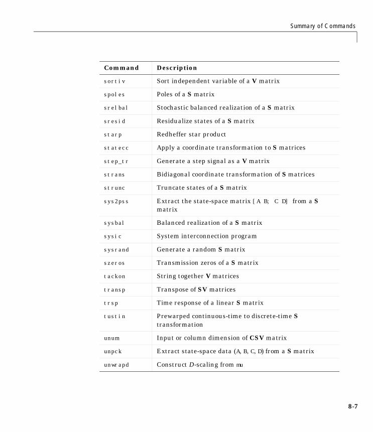
Summary of Commands
sortiv Sort independent variable of a V matrix
spoles Poles of a S matrix
srelbal Stochastic balanced realization of a S matrix
sresid Residualize states of a S matrix
starp Redheffer star product
statecc Apply a coordinate transformation to S matrices
step_tr Generate a step signal as a V matrix
strans Bidiagonal coordinate transformation of S matrices
strunc Truncate states of a S matrix
sys2pss Extract the state-space matrix [A B; C D] from a Smatrix
sysbal Balanced realization of a S matrix
sysic System interconnection program
sysrand Generate a random S matrix
szeros Transmission zeros of a S matrix
tackon String together V matrices
transp Transpose of SV matrices
trsp Time response of a linear S matrix
tustin Prewarped continuous-time to discrete-time Stransformation
unum Input or column dimension of CSV matrix
unpck Extract state-space data (A,B,C,D) from a S matrix
unwrapd Construct D-scaling from mu
Command Description
8-7

8 Reference
8-8
unwrapp Construct ∆ perturbation from mu
vabs Absolute value of a CV matrix
var2con Convert a V matrix to a C matrix
varyrand Generate a random V matrix
vceil Round elements of CV matrices towards ∞
vcjt Conjugate transpace of CV matrices
vdcmate Decimate a V matrix
vdet Determinant of CV matrices
vdiag Diagonal of CV matrices
vebe Element-by-element operations on V matrices
veig Eigenvalue decomposition of CV matrices
veval Evaluate general functions of V matrices
vexpm Exponential of CV matrices
vfind Find individual elements of a V matrix
vfft FFT for V matrices
vfloor Round elements of CV matrices towards –∞
vifft Inverse FFT for V matrices
vimag Imaginary part of a CV matrix
vinterp Interpolate V matrices
vinv Inverse of a CV matrix
vldiv Left division of CV matrices
vnorm Norm of CV matrices
vpck Pack a V matrix
Command Description

Summary of Commands
vpinv Pseudoinverse of a CV matrix
vplot Plot CV matrices
vpoly Characteristic polynomial of CV matrices
vrcond Condition number of a CV matrix
vrdiv Right division of CV matrices
vreal Real part of a CV matrix
vrho Spectral radius of a CV matrix
vroots Polynomial roots of CV matrices
vschur Schur form of a CV matrix
vspect Signal processing spectrum command for V matrices
vsvd Singular value decomposition of a CV matrix
vtp Transpose of CV matrices
vunpck Unpack a V matrix
vzoom Mouse-driven axis selection of plot window
wcperf Worst-case performance for given uncertainty level
wsgui A MATLAB workspace GUI
xnum State dimension of a S matrix
xtract Extract portions of a V matrix using independentvariables
xtracti Extract portions of a V matrix
ynum Output or row dimension of a CSV matrix
zp2sys Convert transfer function poles and zeros into a S matrix
Command Description
8-9

8 Reference
8-1
Commands Grouped by Function
Standard Operations/Basic Functions
abv Stack CSV matrices above one another
cjt Conjugate transpose of SV matrices
daug Diagonal augmentation of CSV matrices
madd Addition of CSV matrices
minv Inverse of CSV matrices
mmult Multiplication of CSV matrices
mscl Scale (by a scalar) a SV matrix
msub Subtraction of CSV matrices
sbs Stack CSV matrices next to one another
sclin Scale S matrix input
sclout Scale S matrix output
sel Select CSV matrix rows/columns or outputs/inputs
starp Redheffer star product
transp Transpose of SV matrices
0
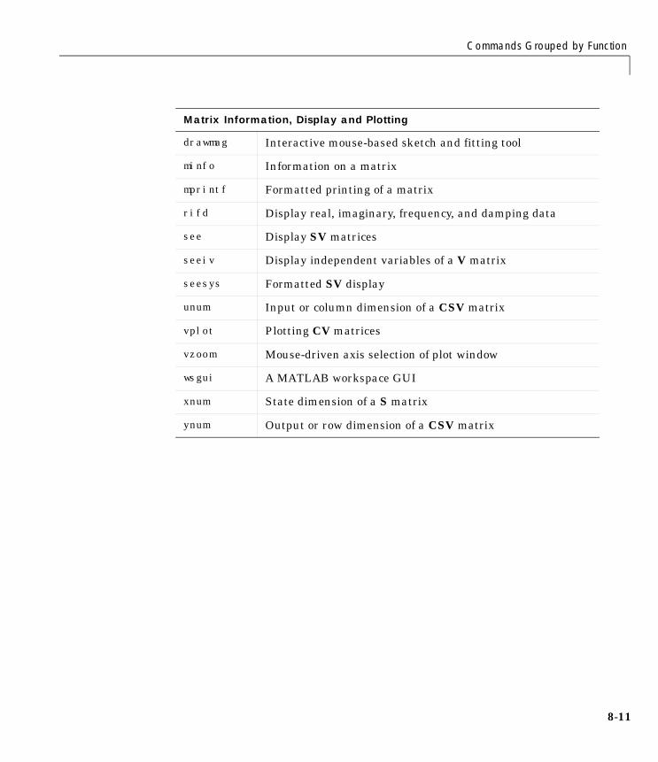
Commands Grouped by Function
Matrix Information, Display and Plotting
drawmag Interactive mouse-based sketch and fitting tool
minfo Information on a matrix
mprintf Formatted printing of a matrix
rifd Display real, imaginary, frequency, and damping data
see Display SV matrices
seeiv Display independent variables of a V matrix
seesys Formatted SV display
unum Input or column dimension of a CSV matrix
vplot Plotting CV matrices
vzoom Mouse-driven axis selection of plot window
wsgui A MATLAB workspace GUI
xnum State dimension of a S matrix
ynum Output or row dimension of a CSV matrix
8-11

8 Reference
8-1
Modeling Functions
mfilter Construct a Bessel, Butterworth, Chebychev, or RC filter
nd2sys Convert a SISO transfer function into a µ-Tools S matrix
pck Create a S matrix from state-space data (A, B, C, D)
pss2sys Convert an [A B;C D] matrix into a µ-Tools S matrix
sys2pss Extract state-space matrix [A B; C D] from a S matrix
sysic System interconnection program
unpck Extract state-space data (A,B,C,D) from a S matrix
zp2sys Convert transfer function poles and zeros to a S matrix
SYSTEM Matrix Functions
reordsys Reorder states in a S matrix
samhld Sample-hold approximation of a continuous S matrix
spoles Poles of a S matrix
statecc Apply a coordinate transformation to S matrices
strans Bidiagonal coordinate transformation of S matrices
sysrand Generate a random S matrix
szeros Transmission zeros of a S matrix
tustin Prewarped continuous to discrete S transformation
2

Commands Grouped by Function
Model Reduction Functions
cf2sys Create a S from a normalized coprime factorization
hankmr Optimal Hankel norm approximation of a S matrix
sdecomp Decompose a S matrix into two S matrices
sfrwtbal Frequency weighted balanced realization of a S matrix
sfrwtbld Stable frequency weighted realization of a S matrix
sncfbal Balanced realization of coprime factors of a S matrix
srelbal Stochastic balanced realization of a S matrix
sresid Residualize states of a S matrix
strunc Truncate states of a S matrix
sysbal Balanced realization of a S matrix
SYSTEM Response Functions
cos_tr Generate a cosine signal as a V matrix
dtrsp Discrete-time response of a linear S matrix
frsp Frequency response of a S matrix
sdtrsp Sample data time response of a linear S matrix
siggen Generate a signal as a V matrix
simgui A GUI for time simulations of LFTs
sin_tr Generate a sine signal as a V matrix
step_tr Generate a step signal as a V matrix
trsp Time response of a linear S matrix
8-13

8 Reference
8-1
H2 and H∞ Analysis and Synthesis Functions
dhfnorm Calculate discrete-time ∞-norm of a stable S matrix
dhfsyn Discrete-time H∞ control design
emargin Normalized coprime factor robust stability margin
gap Calculate the gap metric between S matrices
h2norm Calculate 2-norm of a stable, strictly proper S matrix
h2syn H2 control design
hinffi H∞ full information control design
hinfnorm Calculate ∞-norm of a stable, proper S matrix
hinfsyn H∞ control design
hinfsyne H∞ minimum entropy control design
ncfsyn H∞ loopshaping control design
nugap Calculate the ν (nu) gap between S matrices
pkvnorm Peak norm of a V matrix
sdhfnorm Sample-data ∞-norm of a stable S matrix
sdhfsyn Sample-data H∞ control design
4

Commands Grouped by Function
Structured Singular Value (µ) Analysis and Synthesis
blknorm Block norm of CV matrices
cmmusyn Constant matrix µ synthesis
dkit Automated D – K iteration for µ synthesis
dkitgui Automated D – K iteration GUI for µ synthesis
dypert Create a rational perturbation from frequency mu data
fitmag Fit magnitude data with real, rational, transfer function
fitmaglp Fit magnitude data with real, rational, transfer function
fitsys Fit frequency response data with transfer function
genphase Generate a minimum phase frequency response to magnitudedata
genmu Real and complex generalized µ-analysis of CV matrices
magfit Fit magnitude data with real, rational, transfer function (abatch process)
mu Real and complex µ-analysis of CV matrices
msf Interactive D-scaling rational fit routine
muftbtch Batch D-scaling rational fit routine
musynfit Interactive D-scaling rational fit routine
musynflp Interactive D-scaling rational fit routine (linear program)
8-15

8 Reference
8-1
muunwrap Construct D-scaling and ∆ perturbation from mu
randel Generate a random perturbation
sisorat Fit a frequency point with first order, all-pass, stable transferfunction
unwrapd Construct D-scaling from mu
unwrapp Construct ∆ perturbation from mu
wcperf Worst-case performance for a given ∆
VARYING Matrix Manipulation
getiv Get the independent variable of a V matrix
indvcmp Compare the independent variable data of two V matrices
scliv Scale the independent variable of a V matrix
sortiv Sort the independent variable of a V matrix
tackon String together V matrices
var2con Convert a V matrix to a C matrix
varyrand Generate a random V matrix
vfind Find individual elements of a V matrix
vpck Pack a V matrix
vunpck Unpack a V matrix
xtract Extract portions of a V matrix
xtracti Extract portions of a V matrix using independent variable
Structured Singular Value (µ) Analysis and Synthesis
6

Commands Grouped by Function
Standard MATLAB Commands for VARYING Matrices
vabs Absolute value of a CV matrix
vceil Round elements of CV matrices towards ∞
vdet Determinant of CV matrices
vdiag Diagonal of CV matrices
veig Eigenvalue decomposition of CV matrices
vexpm Exponential of CV matrices
vfft FFT for V matrices
vfloor Round elements of CV matrices towards –∞
vifft Inverse FFT for V matrices
vimag Imaginary part of a CV matrix
vinv Inverse of a CV matrix
vnorm Norm of CV matrices
vpinv Pseudoinverse of a CV matrix
vpoly Characteristic polynomial of CV matrices
vrcond Condition number of a CV matrix
vreal Real part of a CV matrix
vroots Polynomial roots of CV matrices
vschur Schur form of a CV matrix
vspect Signal processing spectrum command for V matrices
vsvd Singular value decomposition of a CV matrix
8-17

8 Reference
8-1
Additional VARYING Matrix Functions
vcjt Conjugate transpose of CV matrices
vdcmate Decimate V matrices
vebe Element-by-element operations on V matrices
veval Evaluate general functions of V matrices
vinterp Interpolate V matrices
vldiv Left division of CV matrices
vrdiv Right division of CV matrices
vrho Spectral radius of a CV matrix
vtp Transpose of CV matrices
Utilities and Miscellaneous Functions
crand Complex random matrix generator (uniform distribution)
crandn Complex random matrix generator (normal distribution)
csord Order complex Schur form matrices
massign Assign a portion of a matrix to another
negangle Calculate angle of matrix elements between 0 and –2π
ric_eig Solve a Riccati equation via eigenvalue decomposition
ric_schr Solve a Riccati equation via real Schur decomposition
8
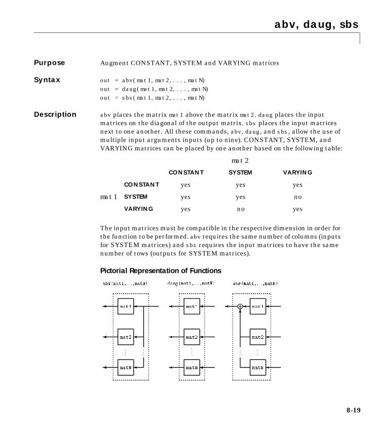
abv, daug, sbs
8abv, daug, sbsPurpose Augment CONSTANT, SYSTEM and VARYING matrices
Syntax out = abv(mat1,mat2,...,matN) out = daug(mat1,mat2,...,matN) out = sbs(mat1,mat2,...,matN)
Description abv places the matrix mat1 above the matrix mat2. daug places the inputmatrices on the diagonal of the output matrix. sbs places the input matricesnext to one another. All these commands, abv, daug, and sbs, allow the use ofmultiple input arguments inputs (up to nine). CONSTANT, SYSTEM, andVARYING matrices can be placed by one another based on the following table:
The input matrices must be compatible in the respective dimension in order forthe function to be performed. abv requires the same number of columns (inputsfor SYSTEM matrices) and sbs requires the input matrices to have the samenumber of rows (outputs for SYSTEM matrices).
Pictorial Representation of Functions
mat1
mat2
CONSTANT SYSTEM VARYING
CONSTANT yes yes yes
SYSTEM yes yes no
VARYING yes no yes
8-19

abv, daug, sbs
Examples Create two CONSTANT matrices a and b along with two SYSTEM matrices p1and p2. Examples of manipulation using abv, daug, and sbs are shown in thefollowing examples:
a = [1 2 3; 4 5 6];b = [7 7 7; 8 8 8 ];pl = pck(–10,1,10,0);p2 = pck(–3,2,4,.1),seesys(abv(p1,p2))
-1.0e+01 0.0e+00 | 1.0e+00 0.0e+00 -3.0e+00 | 2.0e+00--------------------------------- 0.0e+01 0.0e+00 | 0.0e+00 0.0e+01 4.0e+00 | 1.0e-00
out = abv(a,b,b)out =
1 2 34 5 67 7 78 8 87 7 78 8 8
out = daug(a,b)out =
1 2 3 0 0 04 5 6 0 0 00 0 0 7 7 70 0 0 8 8 8
8-20
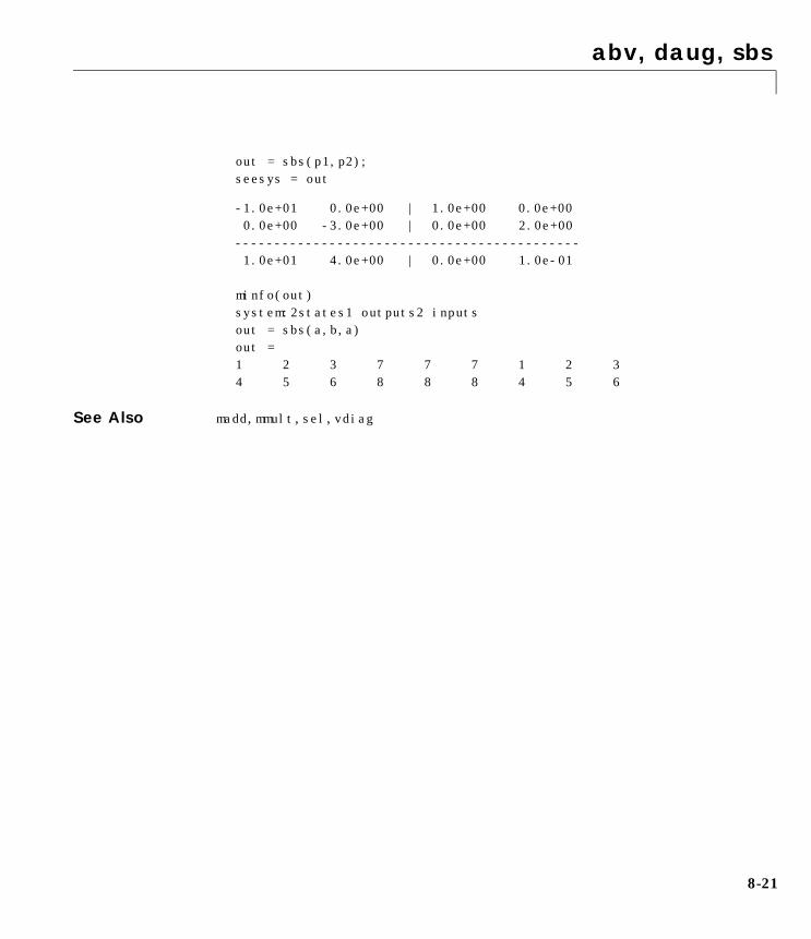
abv, daug, sbs
out = sbs(p1,p2);seesys = out
-1.0e+01 0.0e+00 | 1.0e+00 0.0e+00 0.0e+00 -3.0e+00 | 0.0e+00 2.0e+00-------------------------------------------- 1.0e+01 4.0e+00 | 0.0e+00 1.0e-01 minfo(out)system:2states1 outputs2 inputsout = sbs(a,b,a)out =1 2 3 7 7 7 1 2 34 5 6 8 8 8 4 5 6
See Also madd, mmult, sel, vdiag
8-21

blknorm
8blknormPurpose Create a matrix which is made up of norms of subblocks. Used in conjunctionwith mu (µ)
Syntax matout = blknorm(matin,blk)
Description blknorm computes the maximum singular value of the subblocks of matin,using the information in the perturbation block structure, blk. The output ofblknorm is matout whose entries are the maximum singular value of thesubblocks of matin with these norms as elements. This helps to show whichparts of the matrix are contributing to making µ large. A more completedescription of the perturbation block structure, blk, can be found with thecommand mu and in Chapter 4. blknorm is best used on scaled matrices fromthe upper bound for µ. Repeated δI blocks are treated the same way as fullblocks. The function blknorm can be applied to both CONSTANT andVARYING matrices.
Examples Create a 4 × 3 random matrix and determine its subblock norms for twodifferent block structures. The first block structure consists of a two elementrepeated block and a 1 × 2 full block. The second block structure consists of a 1× 1 block, a 1 × 2 full block, and a 1 × 1 block.
m = crand(4,3);disp(m)
0.7012 + 0.9826i 0.0475 + 0.0727i 0.7564 + 0.4364i0.9103 + 0.7227i 0.7361 + 0.6316i 0.9910 + 0.7665i0.7622 + 0.7534i 0.3282 + 0.8847i 0.3653 + 0.4777i0.2625 + 0.6515i 0.6326 + 0.2727i 0.2470 + 0.2378i
disp(blknorm(m,[2 0; 1 2]))1.8498 1.52721.6656 0.6923
mprintf(blknorm(m,[1 1; 1 2; 1 1]), '%6.2f')1.21 0.09 0.871.58 1.35 1.390.70 0.69 0.34
8-22

blknorm
Algorithm The maximum singular value of each block associated with the blk structureis calculated via the MATLAB norm.
See Also mu, norm, vnorm
8-23

cjt, transp, vcjt, vtp
8cjt, transp, vcjt, vtpPurpose Transpose and conjugate transpose of CONSTANT, SYSTEM and VARYINGmatrices
Syntax out = cjt(mat) out = transp(mat) out = vcjt(mat) out = vtp(mat)
Description cjt forms the complex conjugate transpose of the input matrix mat and transpforms the transpose of mat. transp outputs similar results to the MATLABcommand .′. These commands also work on SYSTEM and VARYING matrices.For consistency in our naming convention, vcjt and vtp are the samecommands as cjt and transp, but work on just CONSTANT and VARYINGmatrices.
For a SYSTEM matrix mat, transp, and cjt are defined as
Examples Create a SYSTEM matrix and calculate its transpose and conjugate transposeusing cjt and transp.
A = [–10 0; 0 3]; B = [1 0 3; 0 2 –9]; C = [10 0; 0 4];D = [0 –.2 –45; .82 0 .1];out = pck(A,B,C,D);seesys (out, '%5 .2g')
–10 0 | 1 0 3 0 3 | 0 2 –9-------------------------------------- 10 0 | 0 –.2 –45 0 4 | .82 0 .1
mat A BC D
=
transp(mat) A.' C.'B. ' D.'
,= cjt(mat) A– ' C– 'B– ' D– '
=
8-24

cjt, transp, vcjt, vtp
x = transp (out);seesys (x, '%5 .2g')
–10 0 | 10 0 0 3 | 0 4--------------------------- 1 0 | 0 .82 0 2 | -.2 0 3 -9 | -45 .1
x = cjt(out);seesys (x, '%5 .2g')
10 0 | -10 0 0 3 | 0 -4--------------------------- 1 0 | 0 .82 0 2 | -.2 0 3 -9 | -45 .1
Algorithm These functions call the MATLAB commands ′ and .′ consistent with the typeof input matrices.
See Also vdiag
8-25

cmmusyn
8cmmusynPurpose Approximately solves the constant-matrix µ-synthesis problem, via theminimization
for given matrices R ∈ Cn×m, U ∈ Cn×r,V ∈ Ct×m, and a set ∆ ⊂ Cm×n.
Syntax [bnd,dvec,gvec,qopt] = cmmusyn(R,U,V,blk);
Algorithm This works for CONSTANT or VARYING data in R, U, and V. If two or morematrices are VARYING, the independent variable values of these matricesmust be the same.
The approximation to solving the constant matrix µ synthesis problem istwo-fold: only the upper bound for µ is minimized, and the minimzation is notconvex, hence the optimum is generally not found. If U is full column rank, orV is full row rank, then the problem can (and is) cast as a convex problem,[PacZPB], and the global optimizer (for the upper bound for µ) is calculated.
The upper bound is returned in bnd, and the optimizing Q is returned in qopt.The scaling matrices associated with the upper bound are in dvec and gvec andmay be unwrapped into block diagonal form using muunwrap.
Reference PacZPB: A. K. Packard, K. Zhou, P. Pandey, and G. Becker, “A collection ofrobust control problems leading to LMI’s,” 30th IEEE Conference on Decisionand Control, pp. 1245–1250, Brighton, UK, 1991.
See Also genmu, mu
minQ Cr t×∈ µ∆ R UQV+( )
8-26

cos_tr, sin_tr, step_tr
8cos_tr, sin_tr, step_trPurpose Generate a VARYING matrix containing a cosine, sine, or step signal at anevenly spaced time interval
Syntax out = cos_tr(freq,mag,tinc,lastt) out = sin_tr(freq,mag,tinc,lastt) out = step_tr(timedata,stepdata,tinc,lastt)
Description cos_tr, sin_tr, and step_tr generate time signals for use with the trsp (timeresponse) command. The following are the input variables provided to cos_trand sin_tr:
Inputs to cos_tr and sin_tr:
Output:
Inputs to step_tr:
Output:
freq frequency of the cosine (sine) signal (radians/second)
mag magnitude of signal
tinc time step (increment)
lastt final time (the signal starts at time t=0)
out time varying matrix of the cosine (sine) signal
timedata time at which step occurs (vector)
stepdata magnitude of step (vector)
tinc time step (increment)
lastt final time (the signal starts at time t=0)
out time varying matrix of steps
8-27

cos_tr, sin_tr, step_tr
Examples Synthesize a cosine signal with a 1 Hz frequency and of magnitude 1.5, 5seconds in length. The time increment is .05 seconds.
out=cos_tr(2*pi,1.5,.05,5); vplt('iv,d',out) grid title('Generate a cosine signal via cos_tr') xlabel('time (seconds)') ylabel('Magnitude')
Algorithm cos_tr and sin_tr call the MATLAB commands cos and sin, respectively.
See Also minfo, siggen, trsp, vpck
-1.5
-1
-0.5
0
0.5
1
1.5
0 0.5 1 1.5 2 2.5 3 3.5 4 4.5 5
Generate a cosine signal via cos_tr
time (seconds)
Mag
nitu
de
8-28

crand, crandn, sysrand, varyrand
8crand, crandn, sysrand, varyrandPurpose Generate a random complex CONSTANT, SYSTEM or VARYING matrix
Syntax out = crand(n,m) out = crandn(n,m) sys = sysrand(nstates,ninputs,noutputs,stabflag) vary = varyrand(rdim,cdim,nindv,ivflg)
Description crand and crandn generate random complex matrices of dimensions n × m,using the MATLAB rand and randn commands, respectively. crand elementsare uniformly distributed and crandn elements are normally distributed.
Inputs to crand and crandn:
Output from crand and crandn:
sysrand generates a random SYSTEM matrix with nstates states, ninputsinputs, and noutputs outputs. Setting the stabflag to 1 will result in a stable,random SYSTEM. The default for stabflag is 0.
varyrand creates a random VARYING matrix with a specified number of rows(rdim), columns (cdim), and independent variable values (nindv). The optionalargument ivflg sorts the independent variables to be monotonicallyincreasing if it is set to 0 (default). Otherwise, if ivflg is set to a nonzero value,no sorting is done.
n number of rows of the output matrix
m number of columns of the output matrix
out an n × m complex matrix of random elements
8-29

crand, crandn, sysrand, varyrand
Examples Create a CONSTANT, complex random matrix and a random SYSTEM matrixusing the commands crand and sysrand
crand(4,3)ans =0.4764 + 0.1622i 0.9017 + 0.1351i 0.4103 + 0.4523i0.3893 + 0.0711i 0.4265 + 0.7832i 0.1312 + 0.8089i0.2033 + 0.3653i 0.1420 + 0.4553i 0.8856 + 0.9317i0.0284 + 0.2531i 0.9475 + 0.3495i 0.0922 + 0.6516i
sys=sysrand(2,4,1);seesys(sys)
0.2190 0.6789 | 0.9347 0.5194 0.0346 0.52970.0470 0.6793 | 0.3835 0.8310 0.0535 0.6711------------------|----------------------------------------0.0077 0.3834 | 0.0668 0.4175 0.6868 0.5890
See Also minfo, pck, pss2sys, rand, randel, sys2pss, unpck, vpck, vunpck
8-30

csord
8csordPurpose Compute an ordered, complex Schur form matrix
Syntax [v,t,flgout,reig_min] = csord(m,epp,flgord,flgjw,flgeig)
Description The csord function produces an ordered, complex Schur form matrix of theinput CONSTANT square matrix m with
The MATLAB function schur is called, which results in an unordered Schurform matrix. The subroutine cgivens forms a complex Givens rotation matrix,which orders the t matrix as you define it. The v matrix is the transformationmatrix. A series of optional input flags can be set:
The output flag flgout is nominally 0. flout is set to 1 if there are jω-axiseigenvalues, set to 2 if there are an unequal number of positive and negativeeigenvalues, or set to 3 if both conditions occur. The fourth output argument,reig_min, is the minimum, magnitude real part of the eigenvalues of m.
epp user-supplied zero tolerance (default epp = 0)
flgord=0
flgord=1
order eigenvalues in ascending real part (default)
partial real part ordering, with real parts less than zero first,then the jω axis eigenvalues and finally the real parts greaterthan zero
flgjw=0
flgjw=1
no exit condition on eigenvalue location (default)
exit if abs(real(eigenvalues(i)))< epp
flgeig=0
flgeig=1
no exit condition on half-plane eigenvalue distribution (default)
exit if length(real(eigenvalues)>0) = length(real(eigenvalues)<0)
tt11 t12
0 t22
==v′ * m * v
8-31

csord
The ric_schr routine calls csord to solve for a stabilizing solution to a matrixRiccati equation. In this case, the m matrix has a special structure, and failuremodes are flagged to avoid extra, unnecessary computations.
Algorithm The eigenvalues are reordered by iterating through each of them andinterchanging them via a bubble sort based on the input flag, flgord. Thesubroutine cgivens exchanges the out of order eigenvalues.
Reference Golub, G.H. and C.F. Van Loan, Matrix Computations, The Johns HopkinsUniversity Press, 1983.
See Also cgivens, ric_schr, rsf2csf, schur
8-32

dhfnorm
8dhfnormPurpose dhfnorm computes the H∞ gain of a stable, discrete-time SYSTEM matrix
Syntax out = dhfnorm(sys,ttol,h,iiloc)
Description dhfnorm computes the H∞ norm of a stable, discrete-time SYSTEM. It convertsthe SYSTEM to continuous-time via a bilinear transformation and then callsthe routine hinfnorm.
The method uses the bilinear transformation from the z-plane to the s-planegiven by,
where h is the time between samples. This is a transformation between theunit disk and the left half plane. If the system p has a pole close to z = –1, thena preliminary output feedback is used to move such poles before the bilineartransformation is performed.
Input arguments:
Output arguments:
Reference Doyle, J.C., K. Glover, P. Khargonekar, and B. Francis, “State-space solutionsto standard H2 and H∞ control problems,” IEEE Transactions on AutomaticControl, vol. 34, no. 8, pp. 831–847, August 1989.
sys SYSTEM matrix (discrete-time), CONSTANT or VARYINGmatrix
ttol relative tolerance of accuracy for SYSTEM matrices only,(default= 0.001)
h time between samples (default 1)
iiloc initial estimate of worst case frequency (optional)
out a 1 × 3 vector giving a lower bound, upper bound andthe frequency where the lower bound occurs.
z 1 sh 2⁄+1 sh 2⁄–-----------------------= , s 2z 1–
hz 1+----------------=
8-33

dhfnorm
See Also hinfsyne, hinffi, hinfnorm, hinfsyn, h2syn, h2norm, ric_eig, ric_schr,sdhfnorm, sdhfsyn
8-34

dhfsyn
8dhfsynPurpose dhfsyn computes an H∞ controller for a discrete-time SYSTEM interconnectionmatrix
Syntax [k,g,gfin,ax,ay,hamx,hamy] = dhfsyn(p,nmeas,ncon,...gmin,gmax,tol,h,z0,quiet,ricmethd,epr,epp)
Description dhfsyn calculates a discrete-time H∞ controller that achieves the infinity normgfin for the interconnection structure p. The controller, k, stablizes thediscrete-time SYSTEM matrix p and has the same number of states as p. TheSYSTEM p is partitioned
where B1 are the disturbance inputs, B2 are the control inputs, C1 are theerrors to be kept small, and C2 are the output measurements provided to thecontroller. B2 has column size (ncon) and C2 has row size (nmeas).
The closed-loop system is returned in g. The same bilinear transformationmethod described for dhfnorm is used. The controller k is returned thatminimizes the entropy integral,
The program calls the continuous-time routine hinfsyne and thecorresponding conditions and tests need to be satisfied.
p
A B1 B2
C1 D11 D12
C2 D21 D22
=
I gfin2
2π-----------– log det
π–
π
∫ I gfin2–
g ejθ( )′g ejθ( )–( ) 1 z02–
–
ejθ z0 1––
2-------------------------------dθ=
8-35

dhfsyn
Input arguments
Output arguments:
p SYSTEM interconnection structure matrix, (stable, discretetime)
nmeas number of measurements output to controller
ncon number of control inputs
gmin lower bound on γ
gmax upper bound on γ
tol relative difference between final γ values
h time between samples (optional)
z0 point at which entropy is evaluated (default ∞)
quiet controls printing on the screen1. no printing0. header not printed–1. full printing (default)
ricmethod 1.Eigenvalue decomposition (with balancing)–1. Eigenvalue decomposition (without balancing)2. Schur decomposition (with balancing, default)–2. Schur decomposition (without balancing)
epr measure of when a real part of an eigenvalue of theHamiltonian matrix is zero (default epr = 1e–10)
epp positive definite determination of the X∞ and Y∞ solution(default epp = 1e–6)
k H∞ (sub) optimal controller (discrete time)
g closed-loop system with H∞ controller (discrete time)
gfin final γ value associated with k and g
ax X∞ Riccati solution as a VARYING matrix with independentvariable γ
8-36

dhfsyn
Note that the outputs ax, ay, hamx, and hamy correspond to the equivalentcontinuous-time problems and can also be scaled and/or balanced.
The dhfsyn program outputs several variables, which can be checked to ensurethat the above conditions are being met. For each γ value the minimummagnitude, real part of the eigenvalues of the X Hamiltonian matrices isdisplayed along with the minimum eigenvalue of X∞, which is the solution tothe X Riccati equation. A # sign is placed to the right of the condition that failedin the printout. This additional information can aid you in the control designprocess.
Algorithm dhfsyn uses the above bilinear transformation to continuous-time and then theformulae described in the Glover and Doyle paper for solution to the optimalH∞ control design problem.
Subroutines called. hinfsyne, hinf_st, hinf_gam, hinfe_c:hinf_gam calls ric_eig, ric_schr, csord, and cgivens
Reference Doyle, J.C., K. Glover, P. Khargonekar, and B. Francis, “State-space solutionsto standard H2 and H∞ control problems,” IEEE Transactions on AutomaticControl, vol. 34, no. 8, pp. 831–847, August 1989.
Glover, K., and J.C. Doyle, “State-space formulae for all stabilizing controllersthat satisfy an H∞ norm bound and relations to risk sensitivity,” Systems andControl Letters, vol. 11, pp. 167–172, 1988.
See Also hinfsyne, hinffi, hinfnorm, hinfsyn, h2syn, h2norm, ric_eig, ric_schr,sdhfnorm, sdhfsyn
ay Y∞ Riccati solution as a VARYING matrix with independentvariable γ
hamx X∞ Hamiltonian matrix as a VARYING matrix withindependent variable γ
hamy Y∞ Hamiltonian matrix as a VARYING matrix withindependent variable γ
8-37

dkit
8dkitPurpose A script file for µ synthesis via D–K iteration
Syntax dkit
Description dkit is a µ-Tools script file for D–K iteration. The D–K iteration procedure isan approximation to µ synthesis control design. It involves a sequence ofminimizations, first over the controller variable K (holding the D variableassociated with the scaled µ upper bound fixed), and then over the D variable(holding the controller K variable fixed). The D–K iteration procedure is notguaranteed to converge to the minimum µ value, but often works well inpractice. A detailed description of the D–K iteration can be found in Chapter 5.
dkit automates the D–K iteration procedure but requires the initialization ofseveral variables. The file dk_defin.m is an example of the informationrequired by dkit. You can copy this file from the µ-Tools subroutine directorymutools/subs and modify it for your application. This file can also be renamed.After renaming, assign the variable DK_DEF_NAME in the MATLAB workspaceto the (character string) name of the new file containing the user-definedvariables for dkit. For example, if the filename containing the setup data ishimat_def.m, then
DK_DEF_NAME = 'himat_def';
should be executed in the MATLAB workspace.
The following is a list of what occurs during a single, complete step of theD–K iteration.
1 Upon running dkit, the program prompts you for starting D–K iterationnumber.Starting mu iteration #:
Type 1 to indicate the first D–K iteration.
2 (In the 1st iteration, this step is skipped.) The µ calculation (from theprevious step) provides a frequency-dependent scaling matrices, Df. Thefitting procedure is interactive (msf), and fits these scalings with rational,stable transfer function matrices, .D s( )
8-38
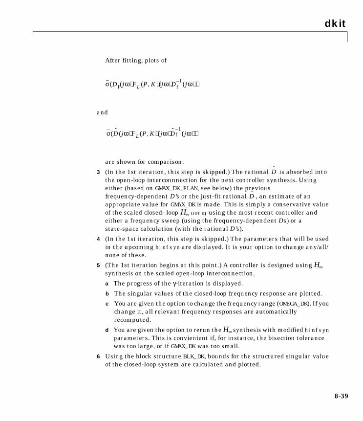
dkit
After fitting, plots of
and
are shown for comparison.
3 (In the 1st iteration, this step is skipped.) The rational is absorbed intothe open-loop interconnnection for the next controller synthesis. Usingeither (based on GMAX_DK_PLAN, see below) the previousfrequency-dependent D’s or the just-fit rational , an estimate of anappropriate value for GMAX_DK is made. This is simply a conservative valueof the scaled closed- loop H∞ norm, using the most recent controller andeither a frequency sweep (using the frequency-dependent Ds) or astate-space calculation (with the rational D’s).
4 (In the 1st iteration, this step is skipped.) The parameters that will be usedin the upcoming hinfsyn are displayed. It is your option to change any/all/none of these.
5 (The 1st iteration begins at this point.) A controller is designed using H∞synthesis on the scaled open-loop interconnection.
a The progress of the γ-iteration is displayed.
b The singular values of the closed-loop frequency response are plotted.
c You are given the option to change the frequency range (OMEGA_DK). If youchange it, all relevant frequency responses are automaticallyrecomputed.
d You are given the option to rerun the H∞ synthesis with modified hinfsynparameters. This is convienient if, for instance, the bisection tolerancewas too large, or if GMAX_DK was too small.
6 Using the block structure BLK_DK, bounds for the structured singular valueof the closed-loop system are calculated and plotted.
σ Df jω( )FL P K,( ) jω( )Df1– jω( )( )
σ D jω( )FL P K,( ) jω( )Df1–
jω( )( )
D
D
8-39

dkit
7 An iteration summary is displayed, showing all of the controller order, aswell as the peak value of µ of the closed-loop frequency responses.
8 The choice of stopping, or performing another iteration is given.
Subsequent iterations proceed along the same lines without the need tore-enter the iteration number. A summary at the end of each iteration isupdated to reflect data from all previous iterations. This often providesvaluable information about the progress of the robust controller synthesisprocedure.
To continue iterating on a problem that was started earlier, make sure therelevent data is in the workspace, run dkit and type the number of theiteration you would like to begin.
The following is a list of the variables that you must set (in either dk_defin fileor the file defined by DK_DEF_NAME) and their meanings:
The following is a list of the optional variables that may be set (in eitherdk_defin file or the file defined by DK_DEF_NAME) and their meanings:
NOMINAL_DK Nominal plant interconnection structure, a µ-ToolsSYSTEM matrix.
NMEAS_DK Number of sensor measurements.
NCONT_DK Number of control inputs.
BLK_DK Block structure forµ calculation, used by mu.
OMEGA_DK Frequency response range.
GMIN_DK Lower bound for first H∞ controller design
GMAX_DK Upper bound for first H∞ controller design
GTOL_DK H∞ bisection tolerance for first iteration
GMAX_DK_PLAN Estimates for GMAX_DK in subsequent iterations are madein three manners. The value of GMAX_DK_PLAN determineswhich formula is used:
0 Use previous GMAX_DK
8-40

dkit
1 use 1.2*pkvnorm(peak_mu_value)
2 use hinfnorm(mmult(dsysL,clp,minv(dsysR)))
8-41

dkit
A number of variables are saved in the workspace after each iteration. Some ofthese variables are required every iteration, hence, it doesn’t make sense torecompute them. The other variables are outputs from the D–K iterationprocedure. The variables saved after each iteration are:
bnds_dk(i) Frequency domain upper and lower bounds for µassociated with the ith iteration. The (i) denotes the ithiteration which is augmented to the name by the programdkit.
dl_dk(i) Left state-space D-scale associated with ith iteration. The(i) denotes the ith iteration which is augmented to thename by the program dkit. Hence, dl_dk5 would be theleft state-space D-scale from the fifth iteration.
dr_dk(i) Right state-space D-scale associated with ith iteration.Same notation.
Dscale_dk(i) D-scaling data output from mu associated with ithiteration. Dscale_dk(i) is in compressed form. Samenotation.
gf_dk(i) The H∞ norm of the ith iteration closed-loop system. Samenotation.
k_dk(i) Controller from the ith iteration. Same notation.
nom_dk_g Frequency response of NOMINAL_DK using OMEGA_DK.
sens_dk(i) Sensitivity data output from the ith iteration mucalculation. Same notation.
8-42

dkit
Fitting D-scalingsThe D-scale fitting procedure is interactive and uses the µ-Tools command msf.During step 2 of the D–K iteration procedure, you are prompted to enter yourchoice of options for fitting the D-scaling data. After pressing return, thefollowing is a list of your options.
Enter Choice (return for list):Choices:nd Move to Next D-Scalingnb Move to Next D-Blocki Increment Fit Orderd Decrement Fit Orderapf Auto-PreFitmx 3 Change Max-Order to 3at 1.01 Change Auto-PreFit tol to 1.010 Fit with zeroth order2 Fit with second ordern Fit with n'th ordere Exit with Current Fittingss See Status
• nd and nb allow you to move from one D-scale data to another. nd moves tothe next scaling, whereas nb moves to the next scaling block. For scalarD-scalings, these are identical operations, but for problems with fullD-scalings, (perturbations of the form δI) they are different. In the (1,2)subplot window, the title displays the D-scaling Block number, the row/column of the scaling that is currently being fit, and the order of the currentfit (with d for data, when no fit exists).
• The order of the current fit can be incremented or decremented (by 1) usingi and d.
• apf automatically fits each D-scaling data. The default maximum state orderof individual D-scaling is 5. The mx variable allows you to change themaximum D-scaling state order used in the automatic prefitting routine. mxmust be a positive, nonzero integer. at allows you to define how close therational, scaled µ upper bound is to approximate the actual µ upper bound ina norm sense. Setting at 1 would require an exact fit of the D-scale data, andis not allowed. Allowable values for at are greater than 1. This setting playsa role (mildly unpredictable, unfortunately) in determining where in the
8-43

dkit
(D,K) space the D–K iteration converges.• Entering a positive integer at the prompt will fit the current D-scale data
with that state order rational transfer function.
• e exits the D-scale fitting to continue the D–K iteration.
• The variable s will display a status of the current and fits.
Examples An example of using dkit for D–K iteration is provided in the “HIMAT RobustPerformance Design Example” in Chapter 7.
Reference Balas, G.J.and J.C. Doyle, “Robust control of flexible modes in the controllercrossover region,” AIAA Journal of Guidance, Dynamics and Control, Vol. 17,no. 2, pp. 370–377, March-April, 1994.
Balas, G.J., A.K. Packard and J.T. Harduvel, “Application of µ-synthesistechniques to momentum management and attitude control of the spacestation,” AIAA Guidance, Navigation and Control Conference, New Orleans,August 1991.
Doyle, J.C., Doyle, K. Lenz, and A. Packard, “Design examples usingµ-synthesis: Space shuttle lateral axis FCS during reentry,” NATO ASI Series,Modelling, Robustness, and Sensitivity Reduction in Control Systems, vol. 34,Springer-Verlag, 1987.
Packard, A., J. Doyle, and G. Balas, “Linear, multivariable robust control witha µ perspective,” ASME Journal of Dynamic Systems, Measurement andControl, 50th Anniversary Issue, vol. 115, no. 2b, pp. 310–319, June 1993.
Stein, G., and J. Doyle, “Beyond singular values and loopshapes,” AIAAJournal of Guidance and Control, vol. 14, no. 1, pp. 5–16, January, 1991.
See Also hinfsyn, hinfnorm, msf, mu
8-44

dkitgui
8dkitguiPurpose A graphical user interface for µ synthesis via D–K iteration
Syntax dkitgui
Description dkitgui is a graphical user interface (GUI) for D–K iteration. The D–Kiteration procedure is an approximation to µ synthesis control design. Itinvolves a sequence of minimizations, first over the controller variable K(holding the D variable associated with the scaled µ upper bound fixed), andthen over the D variable (holding the controller K variable fixed). The D–Kiteration procedure is not guaranteed to converge to the minimum µ value, butoften works well in practice. A more detailed description of the D–K iterationcan be found in Chapter 5.
The GUI tool, dkitgui, has five windows. They are:
• Main Iteration window, which is the main interface for the user during theiteration.
• Setup window, where initial data is entered.• Parameter window, which is occasionally used to modify properties of the
D–K iteration, such as H∞ parameters, and to select the variables that areautomatically exported to the workspace each iteration.
• Frequency Response window, where the plots of µ and of the closed-looptransfer function matrix are displayed.
• Scaling window, where the rational fits of the frequency-dependent D-scaledata are shown, and can be modified.
dkitgui completely automates the D–K iteration procedure. A detaileddescription of dkitgui and its use can be found in Chapter 5.
Examples An example of using dkitgui for D–K iteration is provided in the “HIMATRobust Performance Design Example” section in Chapter 7.
Reference Balas, G.J.and J.C. Doyle, “Robust control of flexible modes in the controllercrossover region,” AIAA Journal of Guidance, Dynamics and Control, vol. 17,no. 2, pp. 370–377, March-April, 1994.
Balas, G.J., A.K. Packard and J.T. Harduvel, “Application of µ-synthesistechniques to momentum management and attitude control of the spacestation,” AIAA Guidance, Navigation and Control Conference, New Orleans,pp. 1204–1213, August 1991.
σ
8-45

dkitgui
Doyle, J.C., Doyle, K. Lenz, and A. Packard, “Design examples using synthesis:Space shuttle lateral axis FCS during reentry,” NATO ASI Series, Modelling,Robustness, and Sensitivity Reduction in Control Systems, vol. 34,Springer-Verlag, 1987.
Packard, A., J. Doyle, and G. Balas, “Linear, multivariable robust control witha perspective,” ASME Journal of Dynamic Systems, Measurement and Control,50th Anniversary Issue, vol. 115, no. 2b, pp. 310–319, June 1993.
Stein, G., and J. Doyle, “Beyond singular values and loopshapes,” AIAAJournal of Guidance and Control, vol. 14, no. 1, pp. 5–16, January, 1991.
See Also dkit, hinfsyn, hinfnorm, mu, pkvnorm
8-46

drawmag
8drawmagPurpose Provide an interactive mouse-based log-log sketch and fitting tool
Syntax [sysout,pts] = drawmag(in,init_pts)
Description drawmag interactively uses the mouse in the plot window to create a VARYINGmatrix pts and a stable, minimum-phase SYSTEM sysout, whichapproximately fits, in magnitude, the frequency VARYING matrix in pts.
Input arguments:
Output arguments:
While drawmag is running, all interaction with the program is through themouse and/or the keyboard. The mouse, if there is one, must be in the plotwindow. The program recognizes several commands:
• Clicking the mouse button adds a point at the crosshairs. If the crosshairsare outside the plotting window, the points will be plotted when the fitting,windowing, or replotting modes are invoked. Typing a is the same as clickingthe mouse button.
• Typing r removes the point with frequency nearest that of the crosshairs.
• Typing any integer between 0–9 fits the existing points with a transferfunction of that order. The fitting routine approximately minimizes themaximum error in a log sense. The new fit is displayed along with the points,and the most recent previous fit, if it exists.
• Typing w uses the crosshair location as the initial point in creating a window.Moving the crosshairs and clicking the mouse or pressing any key then givesa second point at the new crosshair location. These two points define a new
in either a VARYING matrix which is plotted each time as areference or a CONSTANT matrix of the form [xmin xmax yminymax] specifying the plot window on the data.
init_pts optional VARYING matrix of initial set of points
sysout SYSTEM matrix fitting pts.
pts VARYING matrix of points.
8-47

drawmag
window on the data, which is immediately replotted. This is useful in finetuning parts of the data. Windowing may be called repeatedly.
• Typing p simply replots the data using a window that covers all the currentdata points as well as whatever was specified in in. Typically used afterwindowing to view all the data.
• Typing k invokes the keyboard using the keyboard command. Cautionshould be exercised when using this option, as it can wreak havoc on theprogram if variables are changed.
See Also axis, ginput, magfitlp, musynfit, vplot
8-48
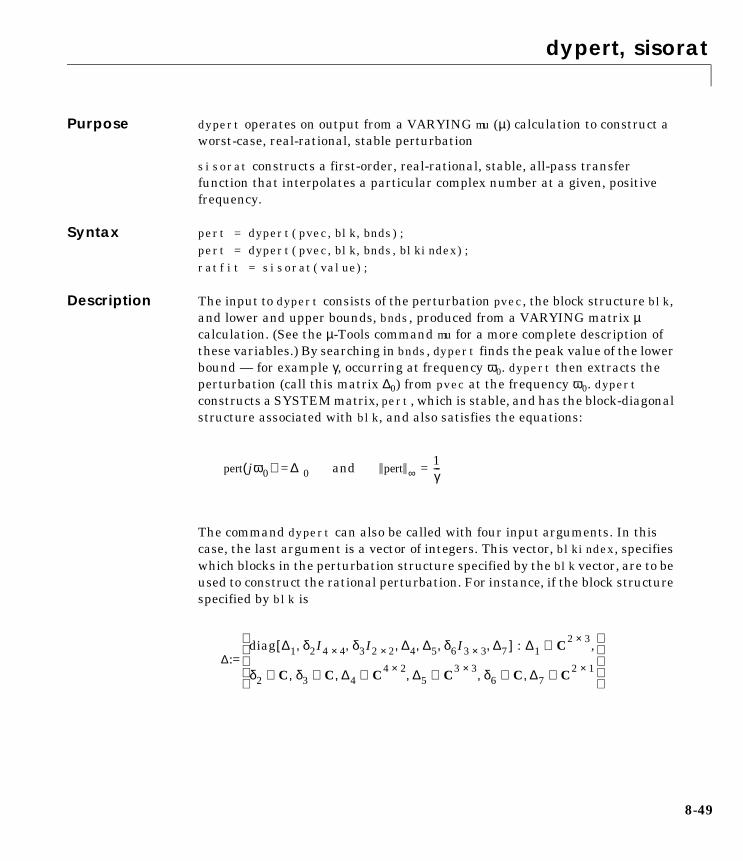
dypert, sisorat
8dypert, sisoratPurpose dypert operates on output from a VARYING mu (µ) calculation to construct aworst-case, real-rational, stable perturbation
sisorat constructs a first-order, real-rational, stable, all-pass transferfunction that interpolates a particular complex number at a given, positivefrequency.
Syntax pert = dypert(pvec,blk,bnds); pert = dypert(pvec,blk,bnds,blkindex); ratfit = sisorat(value);
Description The input to dypert consists of the perturbation pvec, the block structure blk,and lower and upper bounds, bnds, produced from a VARYING matrix µcalculation. (See the µ-Tools command mu for a more complete description ofthese variables.) By searching in bnds, dypert finds the peak value of the lowerbound — for example γ, occurring at frequency ω0. dypert then extracts theperturbation (call this matrix ∆0) from pvec at the frequency ω0. dypertconstructs a SYSTEM matrix, pert, which is stable, and has the block-diagonalstructure associated with blk, and also satisfies the equations:
The command dypert can also be called with four input arguments. In thiscase, the last argument is a vector of integers. This vector, blkindex, specifieswhich blocks in the perturbation structure specified by the blk vector, are to beused to construct the rational perturbation. For instance, if the block structurespecified by blk is
pert jω0( ) ∆0 and pert ∞ = 1γ---=
∆:=diag ∆1 δ2I4 4× δ3I2 2× ∆4 ∆5 δ6I3 3× ∆7, , , , , ,[ ] : ∆1 C2 3× ,∈
δ2 C∈ δ3 C∈ ∆4 C4 2×∈ ∆5 C3 3×∈ δ6 C∈ ∆7 C2 1×∈, , , , ,
8-49

dypert, sisorat
and the fourth argument to dypert is [3 6 4 1] (indicating first, third, fourth,and sixth blocks are desired), then the output SYSTEM matrix produced bydypert will be a SYSTEM matrix that looks like
This is useful when some of the perturbations are not physical perturbations,but correspond to performance objectives, and hence do not need to beconstructed. Note that regardless of the order in which the numbers occur inthe fourth argument, the perturbations in the output SYSTEM pert are inascending order. When dypert is called with three arguments, all theperturbations are constructed.
The command sisorat is essentially a scalar version of dypert, and is the mainsubroutine for dypert. The input to sisorat is value, a 1 × 1, VARYINGmatrix, with one independent variable value. The independent variable isinterpreted as a frequency, ω0, and the numerical value of value at thatfrequency is denoted by γ. The output of sisorat is a single-input/single-outputstable, real, SYSTEM matrix, ratfit, satisfying:
Algorithm The main subroutine of dypert is sisorat, which operates on the followingfact: for any complex number γ, and any real frequency ω0 > 0, there is a realnumber β > 0 such that by proper choice of sign, the equality
∆1 s( ) 02 2× 02 2× 02 3×
02 3× δ3 s( )I2 2× 02 2× 02 3×
04 3× 04 3× ∆4 s( ) 04 3×
03 3× 03 3× 03 2× δ6 s( )I3 3×
ratfit jω0( ) γ and ratfit jω( ) γ ω∀==
± γ s β–s β+------------
s jω0=γ=
8-50

dypert, sisorat
holds. This is exactly how sisorat works.
In order to understand how dypert works, recall in Chapter 4, the section“Complex Structured Singular Value,” Remark 1 after Definition 2.1. There itwas shown that each full block of a perturbation that causes singularity can infact be chosen to be a dyad, and the program mu does this at each independentvariable value. Hence, the matrix ∆0, as described above, is a diagonalaugmentation of scalar blocks, and dyads. Given that the ith block is a dyad,write it as for complex vectors yi and xi. Using several calls tosisorat, it is possible to create two stable, rational vectors h(s) (column) andr(s) (row), such that each element of the vectors is of the form generated bysisorat (stable, and flat across frequency), and for each k and l
If we define then it is stable, and
Performing this on a block-by-block basis produces the entire rationalperturbation. For the case of a repeated scalar block, that part of theperturbation is constructed directly with one call to sisorat and diagonallyaugmented as many times as needed.
See Also mu, randel, svd, vsvd
∆0iyixi
*=
hk jω0( ) yikjω0( ) rl jω0( ) xil
jω0( )=,=
∆i s( ) := h s( )r s( )
∆i ∞ σ= ∆0i( ) , ∆i jω0( ) ∆0i
=
8-51

fitmag, genphase, fitmaglp, magfit
8fitmag, genphase, fitmaglp, magfitPurpose Fit single-input/single-output magnitude data with a real, rational, minimumphase transfer function
Syntax sys = fitmag(magdata,weight,heading,oldfit,...dmdi,upbd,blk,blknum)
resp = genphase(d) sys = fitmaglp(magdata,weight,heading,oldfit,...
dmdi,upbd,blk,blknum) [sys,fit] = magfit(magdata,dim,weight)
Description fitmag fits a stable, minimum phase transfer function to magnitude data,magdata, with a supplied frequency domain weighting function, weight. Bothof these are VARYING matrices, with identical independent variable values.fitmag uses genphase to generate phase data, and fitsys to do the fit.
genphase uses the complex-cepstrum algorithm to generate a complexfrequency response, resp, whose magnitude is equal to the real, positiveresponse d, but whose phase corresponds to a stable, minimum phase function.
fitmaglp has the same inputs, outputs, and user interaction as fitmag , butuses a linear programming approach to do the fitting instead of fitsys andgenphase.
fitmag and fitmaglp have the additional input arguments dmdi, upbd, blk,and blknum. These arguments are used exclusively with D–K iteration whencalled by musynfit and musynflp. In this case, the magdata is the dvec outputof the mu program and corresponds to the blknum’th frequency varying D scaleto be fit. weight corresponds to a measure of the sensitivity of mu to changes inthe D scales at each frequency. This is the sens output from mu. heading is astring variable denoting the title of the plot and oldfit is usually the D scalingsfrom the previous D–K iteration.
dmdi represents the VARYING matrix analyzed using mu. upbd is the upperbound calculated using mu of dmdi with the perturbation block structure blk.The last argument, blknum, corresponds to the current D scale in the blockstructure being fit with fitmag or fitmaglp. Upon fitting the magnitude data,magdata, the resulting transfer function sys is absorbed into the originalmatrix dmdi and plotted along with the mu upper bound on the lower graph.
8-52
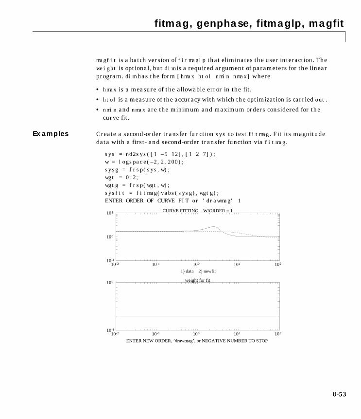
fitmag, genphase, fitmaglp, magfit
magfit is a batch version of fitmaglp that eliminates the user interaction. Theweight is optional, but dim is a required argument of parameters for the linearprogram. dim has the form [hmax htol nmin nmax] where
• hmax is a measure of the allowable error in the fit.
• htol is a measure of the accuracy with which the optimization is carried out.
• nmin and nmax are the minimum and maximum orders considered for thecurve fit.
Examples Create a second-order transfer function sys to test fitmag. Fit its magnitudedata with a first- and second-order transfer function via fitmag.
sys = nd2sys([1 –5 12],[1 2 7]); w = logspace(–2,2,200); sysg = frsp(sys,w); wgt = 0.2; wgtg = frsp(wgt,w); sysfit = fitmag(vabs(sysg),wgtg); ENTER ORDER OF CURVE FIT or 'drawmag' 1
10-1
100
101
10-2 10-1 100 101 102
1) data 2) newfit
CURVE FITTING, W/ORDER = 1
10-1
100
10-2 10-1 100 101 102
weight for fit
ENTER NEW ORDER, ’drawmag’, or NEGATIVE NUMBER TO STOP
8-53

fitmag, genphase, fitmaglp, magfit
A first-order fit does not accurately respresent the frequency data as shown inthe above figure. The solid line represents the curve fit and the dashed linerepresents the original frequency data. You can try and fit the data again witha second-order system.
ENTER ORDER, 'drawmag', or NEGATIVE TO STOP 2
ENTER ORDER, 'drawmag', or NEGATIVE TO STOP –1
The second-order fit lies directly on top of the original data, hence it is difficultto distinguish the two plots. A –1 is entered at the end of this iterationprocedure to indicate satisfaction with the results.
Algorithm The algorithm for fitmag is as follows. On a log-log scale, the magnitude datais interpolated linearly, with a very fine discretization. Then, using thecomplex cepstrum algorithm, the phase, associated with a stable, minimumphase, real, rational transfer function with the same magnitude as the magdatavariable is generated. This involves two fft’s, and logarithmic/exponentialconversions. With the new phase data, and the input magnitude data, theMATLAB function invfreqs is used to find a real, rational transfer functionthat fits the data. heading is an optional title and oldfit is an optional
100
101
10-2 10-1 100 101 102
1) data 2) newfit
CURVE FITTING, W/ORDER = 2
10-1
100
10-2 10-1 100 101 102
weight for fit
ENTER NEW ORDER, ’drawmag’, or NEGATIVE NUMBER TO STOP
8-54

fitmag, genphase, fitmaglp, magfit
previous fit that can be added to the graphs if they are included. These optionsare used in the program musynfit.
The algorithm for magfit is as follows. The system sys is derived by solving alinear program and searching over a parameter h according to the followingspecification. Let m be the given magnitude data, g the transfer function of sysand w the values of weight; then h is found such that at each frequency,
where
The order of sys is increased until an h less than hmax is obtained or nmax isreached. The minimum value of h at this order is then determined to anaccuracy of htol.
Problems For problems with very coarse data, fitmag may give incorrect answers, evenif the data was generated by taking the frequency response of a linear system.The inaccuracy arises in the log-log interpolation step, which is used in thephase calculation. This step is avoided in magfit. Hence, for coarse data sets,magfit should be used. fitmaglp and magfit appear to be sometimes slowerthan fitmag.
Reference Oppenheim, A.V., and R.W. Schaffer, Digital Signal Processing, Prentice Hall,New Jersey, 1975, pp. 513.
See Also fitsys, invfreqs, musynfit, musynflp, muftbtch
1 r⁄ gm----- r,< <
r 1 h w2⁄+= .
8-55

fitsys
8fitsysPurpose Fits single-input/single-output (SISO), single-input/multi-output (SIMO) andmulti-input/single-output (MISO) frequency response data with SYSTEMmatrix
Syntax sys = fitsys(resp,ord,wt,code)
Description fitsys fits frequency response (VARYING) data in resp with a transferfunction of order ord, using a frequency dependent weight in wt (optional). Thefrequency response data may be either a row (SIMO) or column (MISO). Theoptional frequency dependent weight is a VARYING matrix. This weight maybe a scalar (1 row, 1 column), or may be the same shape as resp.
The fourth argument, code, is optional. If set to 0 (default), then the fit is asdescribed. If code = 1, as in the µ-synthesis routines, it forces the fit to be stable,minimum phase, simply by reflecting the poles and zeros if necessary. In thiscase, the response resp comes from the program genphase and alreadycorresponds to a stable, minimum phase transfer function. fitsys is called byfitmag and msf.
Examples An example of how to use fitsys to derive a SIMO transfer function model isprovided in the “More Sophisticated SYSTEM Functions” section in Chapter 2.
Algorithm The author of fitsys is Xin Hua Yang.
See Also fitmag, genphase, msf, vspect
8-56

frsp
8frspPurpose Calculate the complex frequency response of a linear system
Syntax out = frsp(sys,omega,T,balflg)
Description frsp calculates the complex frequency response of a given SYSTEM matrix(sys) for a vector of frequency points (omega). The output matrix out is afrequency dependent VARYING matrix containing the frequency response ofthe input system sys at the frequency values contained in the vector omega .For systems with multiple inputs and outputs, a multivariable frequencyresponse is returned.
Input arguments:
Output arguments
The vector of frequency points is assumed to be real and can be generated fromthe MATLAB command logspace or linspace. Given a continuous system sys,of the form
and an input vector, omega , with N frequencies, [ω1, ω2,. . .,ωN], frsp evaluatesthe following equation
sys SYSTEM matrix
response calculated at these frequencies. If another VARYINGmatrix is input here, then its independent variables are used
T 0 (default) indicates a continuous system. A nonzero value forcesdiscrete system evaluation with sample time T (optional)
balflg 0 (default) balances the SYSTEM A matrix prior to evaluation. Anonzero value for balflg leaves the state-space data unchanged(optional)
out VARYING frequency response matrix
sys A BC D
=
8-57

frsp
C(jωiI – A)–1B + D, i = 1,. . .,N
You can specify a discrete time evaluation by specifying an optional samplingtime, T. For the discrete time case each matrix in the VARYING output is givenby
Note that setting T = 0 implies that a continuous frequency response is to beperformed and not to evaluate
Examples The SYSTEM matrix sys is constructed to have two inputs and two outputswith poles at –2 and –10. A frequency vector omega is constructed with 30points log spaced between .1 and 100 rad/s. The complex frequency response ofsys is calculated and its values between 3.5 and 4.6 rad/s are displayed.
a = [–2 0;0 –10];b = [.2 .12; -.3 .4];c = [.3 .7; 2 –1]; sys = pck(a,b,c); omega = logspace(–1,2,30); sysg = frsp(sys,omega); see(xtract(sysg,3.5,4.6))2 rows 2 columns
iv = 3.56225
–0.0114 – 0.0062i 0.0292 – 0.0165i 0.0746 – 0.0949i –0.0067 – 0.0386i
iv = 4.52035
–0.0125 – 0.0032i 0.0262 – 0.0172i 0.0577 – 0.0853i –0.0136 – 0.0294i
C ejωiT A–( )
1–B D i 1 … N, ,=,+
C ejω i0 A–( )
1–B D+
8-58

frsp
A frequency response is performed using frsp with the default variables set. Aplot of the frequency response is shown with the four line types correspondingto the sysg(1,1), sysg(1,2), sysg(2,1), and the sysg(2,2) elements.
vplot('bode',sysg); title('Complex frequency response example – continuous time')
To demonstrate the calculation of a discrete frequency response, convert thissystem into a digital system via the bilinear transformation. The samplefrequency is chosen as 100 radians/second.
T = 2*pi/100; dsys = tustin(sys,T); omega = sort([omega,logspace(0,2,60)]); dsysg = frsp(dsys,,T); vplot('bode',sysg); title('Complex frequency response example – discrete time')
For digital filter design, you can examine the transfer function from 0 to π byspecifying T = 1. A Chebyshev type II filter is designed and its magnitude isplotted to demonstrate this feature.
10-3
10-2
10-1
100
10-1 100 101 102
Log
Mag
nitu
de
Frequency (radians/sec)
-4
-2
0
2
4
10-1 100 101 102
Pha
se (
radi
ans)
Frequency (radians/sec)
Complex frequency response example - continuous time
8-59
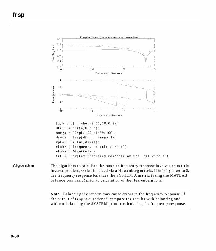
frsp
[a,b,c,d] = cheby2(11,30,0.3); dfilt = pck(a,b,c,d); omega = [0:pi/100:pi*99/100]; dsysg = frsp(dfilt, omega,1); vplot('iv,lm',dsysg); xlabel('frequency on unit circle') ylabel('Magnitude') title('Complex frequency response on the unit circle')
Algorithm The algorithm to calculate the complex frequency response involves an matrixinverse problem, which is solved via a Hessenberg matrix. If balflg is set to 0,the frequency response balances the SYSTEM A matrix (using the MATLABbalance command) prior to calculation of the Hessenberg form.
Note: Balancing the system may cause errors in the frequency response. Ifthe output of frsp is questioned, compare the results with balancing andwithout balancing the SYSTEM prior to calculating the frequency response.
10-5
10-4
10-3
10-2
10-1
100
10-1 100 101 102
Log
Mag
nitu
de
Frequency (radians/sec)
-4
-2
0
2
4
10-1 100 101 102
Pha
se (
radi
ans)
Frequency (radians/sec)
Complex frequency response example - discrete time
8-60

frsp
Reference Laub, A.J., “Efficient Multivariable Frequency Response Computations,” IEEETransactions on Automatic Control, vol. AC–26, No. 2, pp. 407–408, April,1981.
See Also balance, hess, samhld, tustin, vplot
10-4
10-3
10-2
10-1
100
0 0.5 1 1.5 2 2.5 3 3.5
frequency on unit circle
Ma
gn
itud
e
Complex frequency response on the unit circle
8-61

gap, nugap
8gap, nugapPurpose gap calculates the gap metric between two SYSTEM matrices
nugap calculates the ν gap between two SYSTEM matrices.
Syntax gap = gap(sys1,sys2, ttol)nugap = nugap (sys1, sys2, ttol)
Description gap and nugap compute the gap and ν gap metrics between two SYSTEMmatrices. Both quantities give a numerical value δ(G0,G1) between 0 and 1 forthe distance between a nominal system sys1 (G0) and a perturbed system sys2(G1). The gap metric was introduced into the control literature by Zames andEl-Sakkary, 1980, and exploited by Georgiou and Smith, 1990. The ν gapmetric was derived by Vinnicombe, 1993. For both of these metrics thefollowing robust performance result holds from Qui and Davidson, 1992, andVinnicombe, 1993:
arcsin b(G1,K1) ≥ arcsin b(G0,K0)– arcsin δ(G0,G1)– arcsin δ(K0,K1)
where
The interpretation of this result is that if a nominal plant G0 is stabilized bycontroller K0, with “stability margin” b(G0,K0), then the stability margin whenG0 is perturbed to G1 and K0 is perturbed to K1 is degraded by no more than theabove formula. Note that 1/b(G,K) is also the signal gain from disturbances onthe plant input and output to the input and output of the controller. The ν gapis always less than or equal to the gap, so its predictions using the aboverobustness result are tighter. To make use of the gap metrics in robust design,weighting functions need to be introduced. In the above robustness result, Gneeds to be replaced by W2GW1 and K by (similarly for G0, G1, K0 andK1). This makes the weighting functions compatible with the weightingstructure in the “Loop Shaping Using H∞ Synthesis” section in Chapter 3.Model reduction of the system model and controller can be performed by usingbalanced truncations or Hankel norm approximation of normalized coprimefactor representations.
b G K,( ) IK
I GK–( ) 1– G I[ ]∞
1–
=
W11– KW2
1–
8-62
gap, nugap
ttol defines the tolerance to which the gap is computed. The default is 0.001.
Algorithm Tryphon Georgiou and Malcolm Smith wrote the gap program.
The computation of the gap amounts to solving 2-block H∞-problems, Georgiou,1988. The particular method used here for solving the H∞-problems is based onGreen et al., 1990. The computation of the nugap uses the method ofVinnicombe, 1993.
Reference Georgiou, T.T., On the computation of the gap metric, Systems Control Letters,vol. 11, pp. 253–257, 1988.
Georgiou, T.T., and M. Smith, “Optimal robustness in the gap metric,” IEEETransactions on Automatic Control, vol. 35, pp. 673–686, 1990.
Green, M., K. Glover, D. Limebeer, and J.C. Doyle, “A J-spectral factorizationapproach to H∞ control,” SIAM J. of Control and Opt., 28(6), pp. 1350–1371,1990.
Qiu, L., and E.J. Davison, “Feedback stability under simultaneous gap metricuncertainties in plant and controller,” Systems Control Letters, vol. 18–1, pp.9–22, 1992.
Vinnicombe, G., “Measuring Robustness of Feedback Systems,” PhDdissertation, Department of Engineering, University of Cambridge, 1993.
Zames, G., and El-Sakkary, “Unstable systems and feedback: The gap metric,”Proceedings of the Allerton Conference, pp. 380–385, Oct., 1980.
See Also dhfnorm, emargin, hinfnorm, ncfsyn, mu
8-63

genmu
8genmuPurpose Compute upper bounds for the mixed (real and complex) generalizedstructured singular value (referred to as generalized mixed µ) of a VARYING/CONSTANT matrix
Syntax [bnd,dvec,gvec,qmat] = genmu(M,C,blk);
Description Generalized µ allows us to put additional constraints on the directions that I –M∆ becomes singular. Given a matrix M ∈ Cn×n, and C ∈ Cm×n, find thesmallest ∆ ∈ ∆ (described by blk) such that
is not full column rank. Specifically, define
This quantity can be bounded above, using standard µ ideas. If there exists amatrix Q such that
µ∆(M + QC) < β
then µ∆(M,C) < β. Hence,
It is possible to compute the optimal matrix Q which minimizes the standard µ upper bound for µ∆(M + QC). The optimization problem can be reformulatedinto an affine matrix inequality, [PacZPB], and solved with a combination of
I ∆M–
C
µ∆ M C,( ) := 1
min σ ∆( ) : δ ∈ ∆ rank I ∆M–
C, n<
-------------------------------------------------------------------------------------------------------
µ∆ M C,( ) min µ∆ M QC+( )Q C
n m×∈
8-64

genmu
heuristics and general purpose AMI solvers. This is how genmu computes theupper bound µ∆(M,C).
The upper bound for µ∆(M,C) is returned in bnd. The scaling matrices D and Gassociated with the upper bound are in packed format, in the matrics dvec andgvec, and can be unwrapped with muunwrap. The Q matrix which mimimizesthe bound is returned in qmat. If either M or C are VARYING matrices, thenthe bound is computed at each value of the independent variable, and theoutput matrices (bnd, dvec, gvec and qmat) are also VARYING matrices.
Reference Pachard, A., K. Zhou, P. Pandey, and G. Becker, “A collection of robust controlproblems leading to LMI’s,” 30th IEEE Conference on Decision and Control, pp.1245–1250, Brighton, UK, 1991.
See Also cmmusyn, mu
8-65
getiv, sortiv, tackon
8getiv, sortiv, tackonPurpose Return, sort, or append the independent variable values of a VARYINGmatrix
Syntax [indv,err] = getiv(mat) getiv(mat) [out,err] = sortiv(mat,sortflg,nored,epp) out = tackon(mat1,mat2)
Description getiv returns the independent variable values of the VARYING matrix mat. Ifthe input matrix mat is a VARYING matrix, the independent variable isreturned as a column vector, indv, and the output err is set to 0. If mat is nota VARYING matrix, then indv is set to empty, and err is set to 1.
sortiv will reorder the independent variable and associated VARYING matrixto be monotonically increasing or decreasing. The optional sortflg is set to 0(default) for monotonically increasing sorting or nonzero for monotonicallydecreasing sorting. sortiv can be used in conjunction with tackon to meshtogether two different VARYING matrices. The optional third input argument,nored, is set to 0 (default) which does not reduce the number of independentvariables even if there are repeated ones. Setting nored to a nonzero valuecauses repeated independent variables to be collapsed down if theircorresponding matrices are the same. If they are not, an error message isdisplayed and only the first independent variable and corresponding matrix iskept. The output argument err, which is nominally 0, is set to 1 if an errormessage is displayed. The optional fourth input argument, epp, is a vector usedfor checking closeness of two variables. If two independent variables are withinepp(1), and the norm of the difference between the two matrices at these pointsis within epp(2), sortiv collapses these two independent variable values downto one. If the two independent variables are within epp(1), and the normcondition is not satisfied, an error message is displayed and out is set to thenull matrix. When nored is nonzero, the default value for epp is [1e – 9;1e – 9].
tackon strings together two VARYING matrices placing mat1 on top of mat2.mat1 and mat2 must have the same row and column dimensions.
8-66

getiv, sortiv, tackon
Examples The frequency response VARYING matrix from the frsp example is atwo-input/two-output matrix containing 30 points. These independentvariables vary from 0.1 rad/sec to 100 rad/sec.
minfo(sysg)varying: 30 pts2 rows2 colsseeiv(sysg)
1.000e–01 1.269e–01 1.610e–01 2.043e–01 2.593e–013.290e–01 4.175e–01 5.298e–01 6.723e–01 8.532e–011.083e+00 1.374e+00 1.743e+00 2.212e+00 2.807e+003.562e+00 4.520e+00 5.736e+00 7.279e+00 9.237e+001.172e+01 1.487e+01 1.887e+01 2.395e+01 3.039e+013.857e+01 4.894e+01 6.210e+01 7.880e+01 1.000e+02
Typing getiv without any arguments outputs a brief description of its callingsequence. All µ-Tools commands have this feature. The xtract commandselects the independent variables between 1 and 5 rad/sec and the getivcommand returns these independent variables from sysg and stores them inindv.
getivusage: [indv,err] = getiv(mat)[indv] = getiv(xtract(sysg,l,5));indv'ans =1.0826 1.3738 1.7433 2.2122 2.80723.5622 4.5204
The sortiv command (with an optional second argument) resorts theindependent variable of the frequency response of sys in decreasing order.
syslg = sortiv (xtract ( sysg ,1 , 5 ) , 1 ) ;seeiv(syslg)
4.520e+00 3.562e+00 2.807e+00 2.212e+00 1.743e+001.374e+00 1.083e+00
Algorithm getiv and sortiv manipulate VARYING matrices.
See Also indvcmp, sort, xtract, xtracti
8-67

h2norm, hinfnorm
8h2norm, hinfnormPurpose Calculate the H2, H∞ norms of a SYSTEM matrix
Syntax out = h2norm(sys) out = hinfnorm(sys,tol)
Description h2norm calculates the 2-norm of a stable, strictly proper SYSTEM matrix. Theoutput is a scalar, whose value is the 2-norm of the system.
The output from hinfnorm is a 1 × 3 vector, out, which is made up (in order) ofa lower bound for ||sys||∞, an upper bound for ||sys||∞, and a frequency, ωo, atwhich the lower bound is achieved.
The ||⋅||∞ norm calculation is an iterative process and requires a test to stop. Thevariable tol specifies the tolerance used to calculate the ||sys||∞. The iterationstops when
(the current upper bound) ≤ (1 + tol) × (the current lower bound).
The default value of tol is 0.001.
Algorithm The H2 norm of a SYSTEM follows from the solution to the Lyapunov equation.
AX + XA′ + BB′ = 0,
with ||sys||2 = trace (CXC′).
Calculation of the H∞ norm requires checking for jω axis eigenvalues of aHamiltonian matrix, Hα, which depends on a parameter α. If Hα has no jω axiseigenvalues, then the ||⋅||∞ norm of the SYSTEM matrix is less than α. If thematrix Hα does have jω axis eigenvalues, then these occur at the frequencieswhere the transfer matrix has a singular value (not necessarily the maximum)equal to α. By iterating, the value of the ||⋅||∞ norm can be obtained.
out(1) σσσσ(sys j out 3( )⋅( ) ) sys ∞ out(2)≤ ≤=
8-68

h2norm, hinfnorm
Reference Boyd, S., K. Balakrishnan and P. Kabamba, “A bisection method for computingthe H∞ norm of a transfer matrix and related problems,” Math Control Signalsand Systems, 2(3), pp. 207–219, 1989.
Boyd, S., and K. Balakrishnan, “A regularity result for the singular values of atransfer matrix and a quadratically convergent algorithm for computing its H∞norm,” Systems and Control Letters, vol. 15–1, 1990.
Bruinsma, O., and M. Steinbuch, “A fast algorithm to compute theH∞ norm ofa transfer function matrix,” Systems and Control Letters, vol. 14, pp. 287–293,1990.
See Also hinfsyn, h2syn, ric_eig, ric_schr
8-69

h2syn
8h2synPurpose Compute the optimal H2 controller given a SYSTEM interconnection matrix
Syntax [k,g,norms,kfi,gfi,hamx,hamy] =h2syn(p,nmeas,ncon,ricmethod)
Description h2syn calculates the H2 optimal controller k and the closed-loop system g forthe linear fractional interconnection structure p. nmeas and ncon are thedimensions of the measurement outputs from p and the controller inputs to p.The optional fourth argument, ricmethod, determines the method used to solvethe Riccati equations. The interconnection structure, p, is defined by
Input arguments
Output arguments
p SYSTEM interconnection structure matrix
nmeas number of measurements output to controller
ncon number of control inputs
ricmethd 1 Eigenvalue decomposition with balancing–1 Eigenvalue decomposition with no balancing
2 Schur decomposition with balancing. (default)–2 Schur decomposition with no balancing.
k H2 optimal controller
g closed-loop system with optimal controller
norms norms of four different quantities, full information control cost(FI), output estimation cost (OEF), disturbance feedforward cost(DFL) and full control cost (FC), norms = [FI OEF DFL FC];
kfi full information/state feedback control law
gfi full information/state feedback closed-loop system
p
A B1 B2
C1 D11 D12
C2 D21 D22
=
8-70
h2syn
The equations and corresponding nomenclature are taken from the Doyle, etal., 1989, reference. The full information cost is given by the
equation The output estimation cost is given
by , where . The disturbance
feedforward cost is , where L2 is defined by
and the full control cost is given by . X2 and Y2 are the
solutions to the X and Y Riccati equations, respectively.
The H2 solution provides an upper bound on γ for use in the hinfsyn program.
Examples Design an H2 optimal controller for a system matrix, himat_icn, with twosensor measurements (nmeas), two error signals, two actuator inputs (ncont),and eight states. himat_icn differs from the SYSTEM interconnectionstructure himat_ic by the fact that the D11 term of himat_ic is set to be zero.The Schur decompostion method, ricmethd = 2, will be used for solution of theRiccati equations. The program outputs the minimum eigenvalue of X2 and Y2during the computation.
nmeas = 2; ncont = 2; ricmethd = 2; minfo(himat_icn)system:8 states6 outputs6 inputs[k,g] = h2syn(himat_icn,nmeas,ncont,ricmethd);minimum eigenvalue of X2: 2.260000e–02minimum eigenvalue of Y2: 2.251670e–02
hamx H2 Hamiltonian matrix
hamy H2 Hamiltonian matrix
trace B1′ X2B1( )( )
12---
trace F2Y2F2′( )( )
12---
F2 =: B2′ X2 D12
′ C1+( )–
trace L2′ X2L2( )( )
12---
Y2C2′ B1D21
′+( )–
trace C1Y2C1′( )( )
12---
8-71

h2syn
The H∞ and H2 norm of the resulting closed-loop system g can be calculated viathe commands hinfnorm and h2norm.
hinfnorm(g)norm between 2.787 and 2.79achieved near 29.9h2norm(g)1.594e+01
Algorithm h2syn is an M-file in µ-Tools that uses the formulae described in the Doyle, etal., 1989, reference for solution to the optimal H2 control design problem. AHamiltonian is formed and solved via a Riccati equation (ric_eig andric_schr). The D matrix associated with the input disturbances and outputerrors is restricted to be zero.
Subroutines called. ric_eig, ric_schr, csord, and cgivens.
Reference Doyle, J.C., K. Glover, P. Khargonekar, and B. Francis, “State-space solutionsto standard H2 and H∞ control problems,” IEEE Transactions on AutomaticControl, vol. 34, no. 8, pp. 831–847, August 1989.
Glover, K., and J.C. Doyle, “State-space formulae for all stabilizing controllersthat satisfy an H∞ norm bound and relations to risk sensitivity,” Systems andControl Letters, 1988. vol. 11, pp. 167–172, August 1989.
See Also hinfsyn, hinffi, h2norm, hinfnorm, ric_eig, ric_schr
8-72

hinffi
8hinffiPurpose Compute H∞ full-information controller for a SYSTEM interconnection matrix
Syntax [k,g,gfin,ax,hamx] = hinffi(p,ncon,gmin,gmax,tol,ricmethd,epr,epp)
Description hinffi calculates an H∞ full information controller that achieves the infinitynorm gfin for the interconnection structure p. The controller, k, stablizes theSYSTEM matrix p and is constant gain. The system p is partitioned:
where B1 are the disturbance inputs, B2 are the control inputs, and C1 are theerrors to be kept small. B2 has the column size ncon. Within the hinffiprogram, the SYSTEM matrix p is augmented with state and disturbancemeasurements; i.e., the identity matrix with size equal to the number of statesof p and the identity matrix with size equal to the number of disturbances. Becareful when closing the loop with the full information controller since theextra measurements are only augmented inside the command hinffi. Theinternal system used for control design is
The controller is returned in k and the closed-loop system is returned in g. Theprogram provides a γ iteration using the bisection method. Given a high andlow value of γ, gmax and gmin, the bisection method is used to iterate on thevalue of γ in an effort to approach the optimal full information H∞ controldesign. If gmax = gmin, only one γ value is tested. The stopping criteria for the
pA B1 B2
C1 D11 D12
=
A B1 B2
C1 D11 D12
I0
0I
00
8-73

hinffi
bisection algorithm requires the relative difference between the last γ valuethat failed and the last γ value that passed be less than tol. You can selecteither the eigenvalue or Schur method with or without balancing for solvingthe Riccati equations. The eigenvalue method is faster but can have numericalproblems, while the Schur method is slower but generally more reliable.
The algorithm employed requires tests to determine whether a solution existsfor a given γ value. epr is used as a measure of when the Hamiltonian matrixhas imaginary eigenvalues and epp is used to determine whether the Riccatisolution is positive semi-definite. The selection of epr and epp should be basedon your knowledge of the numerical conditioning of the interconnectionstructure p. The conditions checked for the existence of a solution are
• H Hamiltonian matrix must have no jω-axis eigenvalues
• the stabilizing solution, X∞ , of the associated Riccati equation must exist,and be must be positive, semi-definite.
Input arguments:
p SYSTEM interconnection structure matrix
ncon number of controller outputs
gmin lower bound on γ
gmax upper bound on γ
tol relative difference between final γ values, iteration stoppingcriteria
ricmethd 1 Eigenvalue decomposition with balancing.–1 Eigenvalue decomposition with no balancing
2 Schur decomposition with balancing (default)–2 Schur decomposition with no balancing
epr measure of when a real eigenvalue of the Hamiltonian matrixis zero (default epr = 1e–10, optional)
epp positive definite determination of the X∞ solution (default epp= 1e–6, optional)
8-74

hinffi
Output arguments:
Note that the outputs ax, ay, hamx, and hamy may correspond to scaled orbalanced data. The following assumptions are made in the implementation ofthe hinfsyn algorithm and must be satisfied:
(i) (A,B2) is stabilizable(ii) D12 is full column rank
(iii) has full column rank for all ω.
where ω denotes the frequency variable.
On return, there must be no jω-axis eigenvalues associated with the HHamiltonian matrices and the eigenvalues of the Riccati solution, X∞, must allbe ≥ 0, for the closed-loop system to be stable and to have an H∞ norm less thanγ. The bisection algorithm iterates on the value of γ to approach the optimal H∞full information controller.
The hinffi program outputs several variables, which can be checked to ensurethat the above conditions are being met. For each γ value the minimummagnitude, real part of the eigenvalues of the H Hamiltonian matrices isdisplayed along with the minimum eigenvalue of X∞, which is the solution tothe Riccati equation. A # sign is placed to the right of the condition that failedin the printout.
Examples Given an interconnection structure sys with one control input, it is desired tosynthesize a full information controller. The upper bound on γ is 1.0 and thelower bound is specified as 0.1. A tolerance of 0.02 is selected for the stopping
k H∞ full information controller
g closed-loop system with H∞ full information controller
gfin final γ achieved
ax Riccati solution as a VARYING matrix with independentvariable γ
hamx Hamiltonian matrix as a VARYING matrix with independentvariable γ
A jωI– B2
C1 D12
8-75

hinffi
condition for the γ iteration and the Schur method is used to solve the Riccatiequations. The command hinffi outputs the display shown for each value of γ.The final γ value achieved is 0.2547.
ncont = 1;% number of control inputs gmin = .1;% minimum gamma value to be tested gmax = 1;% maximum gamma value to be tested tol = .02;% tolerance on the gamma stopping value ricmethd = 2;% Riccati solution via the Schur method seesys(p)% plant interconnection structure
p =3 1 | 40 0 | 1-------------1 0 | 0
[k,g,gf,ax,hx] = hinffi(p,1,.1,1,.02,2);Test bounds:0.1000<gamma<=1.0000
gamma ham_eig x_eig pass/fail1.000 4.90e+00 5.27e–01 pass0.550 4.66e+00 6.03e–01 pass0.325 3.94e+00 1.06e+00 pass0.213 1.69e+00 –7.63e–01# fail0.269 3.34e+00 2.94e+00 pass0.241 2.78e+00 –4.55e+00# fail0.255 3.10e+00 1.04e+01 pass
Gamma value achieved:0.2547
Algorithm hinffi uses the formulas similar to the ones described in the Glover and Doyle,1988 paper for solution to the H∞ control design problem. See the hinfsyncommand for more information.
Subroutines called. hinffi_t, hinffi_p, hinffi_c, and hinffi_ghinffi_g calls: ric_eig, ric_schr, csord, and cgivens
Reference Doyle, J.C., K. Glover, P. Khargonekar, and B. Francis, “State-space solutionsto standard H2 and H∞ control problems,” IEEE Transactions on AutomaticControl, vol. 34, no. 8, pp. 831–847, August 1989.
8-76

hinffi
Glover, K., and J.C. Doyle, “State-space formulae for all stabilizing controllersthat satisfy an H∞ norm bound and relations to risk sensitivity,” Systems andControl Letters, vol. 11, pp. 167–172, 1988.
See Also h2syn, h2norm, hinfsyn, hinfsyne, hinfnorm, ric_eig, ric_schr
8-77
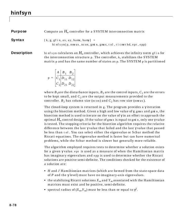
hinfsyn
8hinfsynPurpose Compute an H∞ controller for a SYSTEM interconnection matrix
Syntax [k,g,gfin,ax,ay,hamx,hamy] = hinfsyn(p,nmeas,ncon,gmin,gmax,tol,ricmethd,epr,epp)
Description hinfsyn calculates an H∞ controller, which achieves the infinity norm gfin forthe interconnection structure p. The controller, k, stabilizes the SYSTEMmatrix p and has the same number of states as p. The SYSTEM p is partitioned
where B1are the disturbance inputs, B2 are the control inputs, C1 are the errorsto be kept small, and C2 are the output measurements provided to thecontroller. B2 has column size (ncon) and C2 has row size (nmeas).
The closed-loop system is returned in g. The program provides a γ iterationusing the bisection method. Given a high and low value of γ, gmax and gmin, thebisection method is used to iterate on the value of γ in an effort to approach theoptimal H∞ control design. If the value of gmax is equal to gmin, only one γ valueis tested. The stopping criteria for the bisection algorithm requires the relativedifference between the last γ value that failed and the last γ value that passedbe less than tol. You can select either the eigenvalue or Schur method theRiccati equations. The eigenvalue method is faster but can have numericalproblems, while the Schur method is slower but generally more reliable.
The algorithm employed requires tests to determine whether a solution existsfor a given γ value. epr is used as a measure of when the Hamiltonian matrixhas imaginary eigenvalues and epp is used to determine whether the Riccatisolutions are positive semi-definite. The conditions checked for the existence ofa solution are:
• H and J Hamiltionian matrices (which are formed from the state-space dataof P and the γ level) must have no imaginary-axis eigenvalues.
• the stabilizing Ricatti solutions X∞ and Y∞ associated with the Hamiltionianmatrices must exist and be positive, semi-definite.
• spectral radius of (X∞,Y∞) must be less than or equal to γ2.
p
A B1 B2
C1 D11 D12
C2 D21 D22
=
8-78

hinfsyn
The selection of epr and epp should be based on your knowledge of thenumerical conditioning of the interconnection structure p. The followingassumptions are made in the implementation of the hinfsyn algorithm andmust be satisfied:
(i) (A,B2) is stabilizable and (C2,A) detectable.
(ii) D12 and D21 have full rank.
(iii) has full column rank for all ω ∈ R.
(iv) has full row rank for all ω ∈ R.
Inputs arguments:
p SYSTEM interconnection structure matrix
nmeas number of measurements output to controller
ncon number of control inputs
gmin lower bound on γ
gmax upper bound on γ
tol relative difference between final γ values
ricmethod 1 Eigenvalue decomposition with balancing2 Schur decomposition with balancing (default)
–2 Schur decomposition with no balancing
epr measure of when a real part of an eigenvalue of theHamiltonian matrix is zero (default epr = 1e–10)
epp positive definite determination of the X∞ and Y∞ solution(default epp = 1e–6)
A jωI– B2
C1 D12
A jωI– B1
C2 D21
8-79

hinfsyn
Output arguments:
Note that the outputs ax, ay, hamx, and hamy correspond to scaled or balanceddata.
The hinfsyn program displays several variables, which can be checked toensure that the above conditions are being satisfied. For each γ value beingtested, the minimum magnitude, real part of the eigenvalues of the X and YHamiltonian matrices are displayed along with the minimum eigenvalue of X∞and Y∞, which are the solutions to the X and Y Riccati equations, respectively.The maximum eigenvalue of X∞Y∞, scaled by γ–2,is also displayed. A # sign isplaced to the right of the condition that failed in the printout.
Note: When a Hamiltonian has repeated eigenvalues, solving the Riccatiequation via the eigenvalue method (ric_eig) may have problems. This is dueto the MATLAB command eig incorrectly selecting the eigenvectorsassociated with the repeated roots.
k H∞ (sub) optimal controller
g closed-loop system with H∞ controller
gfin final γ achieved
ax X∞ Riccati solution as a VARYING matrix with independentvariable γ
ay Y∞ Riccati solution as a VARYING matrix with independentvariable γ
hamx H∞ Hamiltonian matrix as a VARYING matrix withindependent variable γ
hamy J∞ Hamiltonian matrix as a VARYING matrix withindependent variable γ
8-80

hinfsyn
Examples This example is taken from the “HIMAT Robust Performance Design Example”section in Chapter 7. himat_ic contains the open-loop interconnectionstructure. Design an H∞ (sub)optimal controller for the SYSTEM matrix,himat_ic, with two sensor measurements, two error signals, two actuatorinputs, two disturbances, and eight states. The range of γ is selected to bebetween 1.0 and 10.0 with a tolerance, tol, on the relative closeness of the finalγ solution of 0.1. The Schur decompostion method, ric_schr, is used forsolution of the Riccati equations. The program outputs at each iteration thecurrent γ value being tested, and eigenvalue information about the H and JHamiltonian matrices and X∞ and Y∞ Riccati solutions. At the end of eachiteration a (p) denoting the tested γ value passed or an (f) denoting a failure isdisplayed. Upon finishing, hinfsyn prints out the γ value achieved.
nmeas = 2;% number of sensor measurements ncont = 2;% number of control inputs gmin = 1;% minimum gamma value to be tested gmax = 10;% maximum gamma value to be tested tol = .1;% tolerance on the gamma stopping value ric = 2;% Riccati equation solved via the Schur method minfo(himat_ic)% SYSTEM interconnection structuresystem: 8 states6 outputs6 inputs
[k,g] = hinfsyn(himat_ic,nmeas,ncon,gmin,gmax,tol,ric);Test bounds: 1.0000 < gamma <=10.0000
gamma hamx_eig xinf_eig hamy_eig yinf_eig nrho_xy p/f10.000 2.3e–02 2.1e–10 2.3e–02 –3.7e–11 0.022 p5.500 2.3e–02 2.1e–10 2.3e–02 –0.0e+00 0.075 p3.250 2.3e–02 2.2e–10 2.3e–02 –0.0e+00 0.222 p2.125 2.3e–02 2.2e–10 2.3e–02 –0.0e+00 0.564 p1.562 2.3e–02 2.4e–10 2.3e–02 –0.0e+00 1.198# f1.844 2.3e–02 2.3e–10 2.3e–02 –0.0e+00 0.789 p1.703 2.3e–02 2.3e–10 2.3e–02 –2.1e–11 0.959 p1.633 2.3e–02 2.3e–10 2.3e–02 –0.0e+00 1.068# f
Gamma value achieved:1.7031
Algorithm hinfsyn uses the formulae described in the Glover and Doyle, 1988, paper forsolution to the optimal H∞ control design problem. There are a number of
8-81

hinfsyn
research issues that need to be addressed for the “best” solution of the Riccatiequations but only two of the standard methods are included.
Subroutines called. hinf_st, hinf_sp, hinf_c, and hinf_gamhinf_gam calls: ric_eig, ric_schr, csord, cgivens
Reference Doyle, J.C., K. Glover, P. Khargonekar, and B. Francis, “State-space solutionsto standard H2 and H∞ control problems,” IEEE Transactions on AutomaticControl, vol. 34, no. 8, pp. 831–847, August 1989.
Glover, K., and J.C. Doyle, “State-space formulae for all stabilizing controllersthat satisfy an H∞norm bound and relations to risk sensitivity,” Systems andControl Letters, vol. 11, pp. 167–172, 1988.
See Also hinffi, hinfnorm, hinfsyne, h2syn, h2norm, ric_eig, ric_schr
8-82

hinfsyne
8hinfsynePurpose Compute an H∞ controller for a SYSTEM interconnection matrix thatminimizes the entropy integral at a specific frequency
Syntax [k,g,gfin,ax,ay,hamx,hamy] = hinfsyne(p,nmeas,ncon,... gmin,gmax,tol,s0,quiet,ricmethd,epr,epp)
Description hinfsyne is a variation of hinfsyn and calculates an H∞ controller thatachieves the infinity norm gfin for the interconnection structure p. Thecontroller, k, stablizes the SYSTEM matrix p and has the same number ofstates as p. Of the controllers achieving this norm bound, k is chosen tominimize an entropy integral relating to the point s0; i.e.,
where g is the closed-loop transfer function. In addition, the amount of printingon the screen can be controlled.
Input arguments:
p SYSTEM interconnection structure matrix
nmeas number of measurements output to controller
ncon number of control inputs
gmin lower bound on γ
gmax upper bound on γ
tol relative difference between final γ values
s0 point at which entropy is evaluated (default ∞)
quiet controls printing on the screen1 no printing1 header not printed
–1 full printing (default)
I gfin2
2π---------------– ln
∞–
∞∫ det I γ 2–
g jω( )′g jω( )–( ) s02
s02 ω2
+----------------------- dω=
8-83
hinfsyne
Output arguments:
Note that the outputs ax, ay, hamx, and hamy correspond to scaled or balanceddata.
The hinfsyne program outputs several variables, which can be checked toensure that the above conditions are being met. For each γ value the minimummagnitude, real part of the eigenvalues of the X Hamiltonian matrices isdisplayed along with the minimum eigenvalue of X∞, which is the solution tothe X Riccati equation. A # sign is placed to the right of the condition that failedin the printout. This additional information can aid you in the control designprocess.
ricmethod 1 Eigenvalue decomposition with balancing–1 Eigenvalue decomposition with no balancing
2 Schur decomposition with balancing (default)–2 Schur decomposition with no balancing
epr measure of when a real part of an eigenvalue of theHamiltonian matrix is zero (default epr = 1e–10)
epp positive definite determination of the X∞ and Y∞ solution(default epp = 1e–6)
k H∞ (sub) optimal controller
g closed-loop system with H∞ controller
gfin final γ value achieved
ax X∞ Riccati solution as a VARYING matrix with independentvariable γ
ay Y∞ Riccati solution as a VARYING matrix with independentvariable γ
hamx H∞ Hamiltonian matrix as a VARYING matrix withindependent variable γ
hamy J∞ Hamiltonian matrix as a VARYING matrix withindependent variable γ
8-84
hinfsyne
Algorithm hinfsyne uses the formulas similar to the ones described in the Glover andDoyle paper for solution to the H∞ control design problem. See the hinfsyncommand for more information.
Subroutines called. hinf_st, hinf_gam, hinfe_c, hinf_gam calls: ric_eig,ric_schr, csord, and cgivens
Reference Doyle, J.C., K. Glover, P. Khargonekar, and B. Francis, “State-space solutionsto standard H2 and H∞ control problems,” IEEE Transactions on AutomaticControl, vol. 34, no. 8, pp. 831–847, August 1989.
Glover, K., and J.C. Doyle, “State-space formulae for all stabilizing controllersthat satisfy an H∞norm bound and relations to risk sensitivity,” Systems andControl Letters, vol. 11, pp. 167–172, 1988.
See Also dhfsyn, hinfsyn, hinffi, hinfnorm, h2syn, h2norm, ric_eig, ric_schr,sdhfsyn
8-85

indvcmp
8indvcmpPurpose Compare the independent variable data of two VARYING matrices
Syntax code = indvcmp(mat1,mat2,errcrit) indvcmp(mat1,mat2,errcrit)
Description indvcmp compares the data for two VARYING matrices. If the two sets ofindependent variables are within a specified tolerance of one another, then theVARYING matrices are assumed to have identical independent variables, andthe VARYING matrices can be combined (i.e., added, subtracted, multiplied,etc.). The results are displayed if an output argument is not provided.
Input arguments:
Output arguments:
Examples Compare the two frequency response matrices, mat has its independentvariable at 0.01 and 0.1 and mat2 has its independent variable at 0.011 and0.1. Given the default comparison criteria, the independent variable isdifferent. Changing the tolerance leads to the command checking differentindvcmp variations in the independent variable.
mat1, mat2= matrices to be compared
errcrit= 1 x 2 optional matrix containing the relative error andabsolute error bounds. The relative error is used to test theerror in independent variables whose magnitude is greaterthan 1e–9, while the absolute error bound used for smallerindependent variable values. Default values are 1e–6, and1e–13, respectively.
code=0code=1code=2code=3
independent variable data is differentindependent variable data is identicaldifferent number of pointsat least one matrix isn’t a VARYING matrix
8-86

indvcmp
see(mat)
2 rows 3 columnsindep variable 0.011 2 34 5 6indep variable 0.1 7 8 910 11 12
see(mat2)
2 rows 3 columnsindep variable 0.01110 20 3040 50 60indep variable 0.1 70 80 90100 110 120
indvcmp(mat,mat2)
varying data is DIFFERENTcode = indvcmp(mat,mat2)
code =0
Changing the relative and absolute error bounds in indvcmp leads these twoindependent variables to be deemed the same.
indvcmp(mat,mat2,[1 1])varying data is the same
Algorithm indvcmp uses standard MATLAB commands.
See Also getiv, sortiv, vunpck, xtract, xtracti
8-87
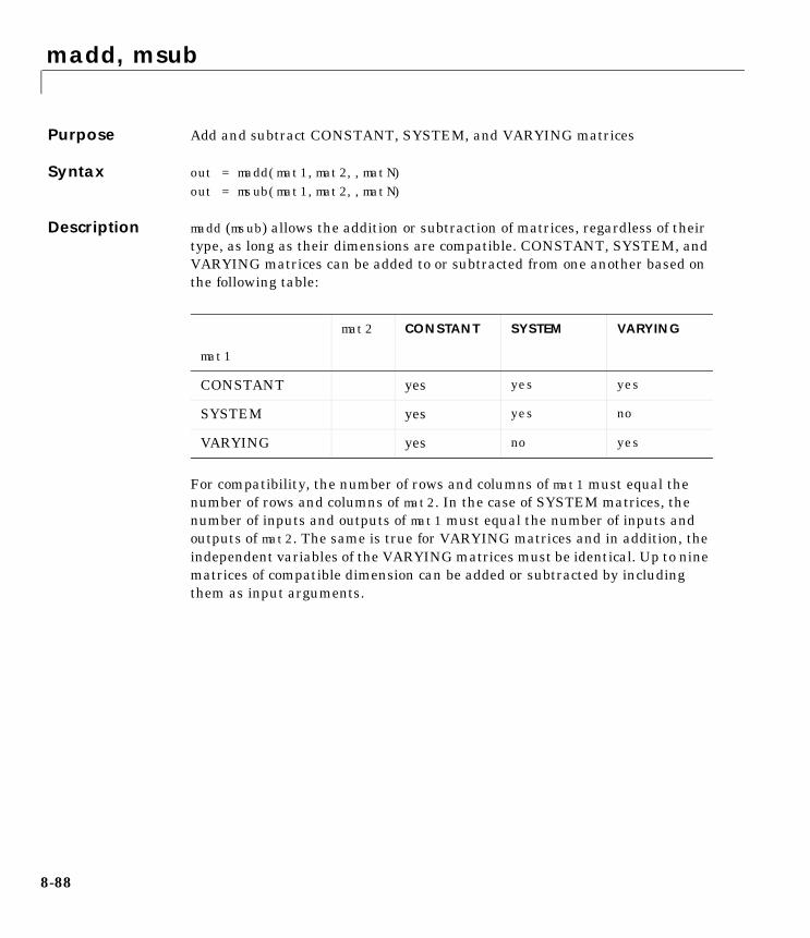
madd, msub
8madd, msubPurpose Add and subtract CONSTANT, SYSTEM, and VARYING matrices
Syntax out = madd(mat1,mat2,,matN) out = msub(mat1,mat2,,matN)
Description madd (msub) allows the addition or subtraction of matrices, regardless of theirtype, as long as their dimensions are compatible. CONSTANT, SYSTEM, andVARYING matrices can be added to or subtracted from one another based onthe following table:
For compatibility, the number of rows and columns of mat1 must equal thenumber of rows and columns of mat2. In the case of SYSTEM matrices, thenumber of inputs and outputs of mat1 must equal the number of inputs andoutputs of mat2. The same is true for VARYING matrices and in addition, theindependent variables of the VARYING matrices must be identical. Up to ninematrices of compatible dimension can be added or subtracted by includingthem as input arguments.
mat2 CONSTANT SYSTEM VARYING
mat1
CONSTANT yes yes yes
SYSTEM yes yes no
VARYING yes no yes
8-88

madd, msub
Pictorial Representationof Functions
Examples Create two SYSTEM matrices p and p1 and a CONSTANT matrix.
a = –10;b = 3;c = 10;d = 0; p = pck(a,b,c,d); minfo(p)system: 1 states 1 outputs 1 inputsa1 = –2; b1 = 3; c1 = 1; d1 = .1; p1 = pck(a1,b1,c1,d1); minfo(p1)seesys(p,'3.2g')
–10 | 3-----|---- 10 | 0
seesys(p1,'3.2g')
–2 | 3----|---- 1 | .1
8-89

madd, msub
Adding two SYSTEM matrices returns a SYSTEM matrix with the samenumber of inputs and outputs as p and p1.
out = madd(p,p1); seesys(out,'3.2g')
–10 0 | 30 –2 | 3---------|------10 1 | .1
minfo(out)system: 2 states 1 outputs 1 inputs
Adding a SYSTEM matrix and a CONSTANT matrix returns a SYSTEMmatrix with the CONSTANT term added to the D-term of the state-spacesystem.
out = madd(p,a); seesys(out,'%3.2g')
-10 | 3------|----- 10 | -10
Subtracting a SYSTEM matrix and a CONSTANT returns a SYSTEM matrixwith the CONSTANT term added to the D-term of the state-space system.
out = msub(p,a); seesys(out,'%3.2g')
-10 | 3------|----- 10 | -10
Algorithm madd and msub call the MATLAB + and – commands consistent with the type ofmatrices.
See Also +, -, mmult, mscl
8-90

massign
8massignPurpose Matrix assignment for VARYING and SYSTEM matrices
Syntax out = massign(matin,rowindex,colindex,data)
Description Performs a matrix assignment like operation on VARYING and SYSTEMmatrices. It is functionally equivalent to:
matin(rowindex,colindex) = data
where rowindex and colindex are vectors specifying the rows and columns (oroutputs and inputs if matin is a SYSTEM) to be changed.
data must either be a constant or of the same type as matin. The dimensions ofdata must be consistent with the lengths of rowindex and colindex.
Note: when applied to a SYSTEM, the result will almost always benonminimal.
Examples In the first example a VARYING matrix with two independent variables isformed with identical (and obvious) data for each matrix.
tl = [11,12,13,14;21,22,23,24;31,32,33,34;41,42,43,44];
vmat = vpck([tl;tl],[0.1,0.2]);
Now make a 2 × 2 data matrix and insert it into the VARYING matrix.Changing the order of the row and column indices has the effect of permutingthe result. This is identical to the constant matrix case.
8-91

massign
ri = [1,3];ci = [4,2];data = [0.001, 0.002; 0.003, 0.004];vmatl = massign(vmat,ri,ci,data);see(vmatl)4 rows 4 columns
iv = 0.1
11.0000 0.0020 13.0000 0.001021.0000 22.0000 23.0000 24.000031.0000 0.0040 33.0000 0.003041.0000 42.0000 43.0000 44.0000
iv = 0.2
11.0000 0.0020 13.0000 0.001021.0000 22.0000 23.0000 24.000031.0000 0.0040 33.0000 0.003041.0000 42.0000 43.0000 44.0000
In the following example part of a system is replaced by the massign function.The initial system is a diagonal system of first order lags. The 2,2 element isreplaced by a lightly damped system and the result plotted. Note that themodified system is no longer minimal.
a = diag([1,2,–3,–4]);b = eye(4);c = diag([1,2,3,4]);sys = pck(a,b,c);subsys = nd2sys(1,[1,0.1,1]);sys = massign(sys,2,2,subsys);minfo(sys)
system: 10 states 4 outputs 4 inputs
omega = logspace(–1,2,100);sys_g = frsp(sys,omega);vplot('liv,lm',sys_g,'–')
8-92
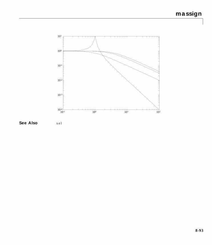
massign
See Also sel
10-4
10-3
10-2
10-1
100
101
10-1 100 101 102
8-93

mfilter
8mfilterPurpose Generate SYSTEM representations of a Bessel, Butterworth, Chebyshev or RCfilter
Syntax sys = mfilter(fc,ord,type,psbndr)
Description Calculates, as a SYSTEM, a single-input, single-output analog low-pass filter.These filters are often encountered in experimental arrangements and must beaccounted for in experimental data processing and control design. For moresophisticated filters see the Signal Processing Toolbox functions.
The cutoff frequency (Hertz) is fc and the filter order is ord. The stringvariable, type, specifies the type of filter and can be one of the following.
The dc gain of each filter (except even order Chebyshev) is set to unity. Theargument psbndr specifies the Chebyshev passband ripple (in dB). At the cutofffrequency, the magnitude is -psbndr dB. For even order Chebyshev filters theDC gain is also -psbndr dB.
The Bessel filters are calculated using the recursive polynomial formula. Thisis poorly conditioned for high order filters (order > 8).
Examples butw = mfilter(2,4,'butterw'); cheb = mfilter(4,4,'cheby',0.5); rc = mfilter(1,4,'rc'); omega = logspace(–1,2,100); butw_g = frsp(butw,omega); cheb_g = frsp(cheb,omega); rc_g = frsp(rc,omega); vplot('bode_gl',[.1 100 .001 10],[.1 100 –180 180],...butw_g,'–',cheb_g,'–',rc_g,'–.')subplot(211),title('Butterworth, RC Chebyshev Filters')
butterw Butterworth
cheby Chebyshev
bessel Bessel
rc series of resistor/capacitor filters
8-94

mfilter
101
100
101
102
300
200
100
0
Pha
se (
degr
ees)
Frequency (radians/sec)
101
100
101
102
102
100
Log
Mag
nitu
de
Frequency (radians/sec)
Butterworth, RC & Chebyshev Filters
8-95
minfo
8minfoPurpose Provide matrix information
Syntax minfo(matin) [systype,rowdata,coldata,pointdata] = minfo(matin)
Description minfo returns information about the data type, and size of the matin. With nooutput assignment, minfo returns text output to the screen. The information isdetermined from the data structure as defined in the “The Data Structures”section in Chapter 2.
With output arguments, minfo returns four arguments. The first argument,systype, is a string variable that can take one of four values. Theinterpretation of the three additional output arguments is based on thevariable systype.
systype == 'vary' matin is a VARYING matrix. pointdata tells howmany independent variable values there are,rowdata is the row dimension of a matrix, andcoldata is the column dimension
systype == 'syst' matin is a SYSTEM matrix. pointdata is thenumber of states, rowdata is the number of outputs,and coldata is the number of inputs.
systype == 'cons' matin is a regular MATLAB matrix, pointdata is setto NaN, rowdata is the number of rows, and coldatais the number of columns.
systype == 'empt' matin is an empty MATLAB matrix; also pointdata,rowdata, and coldata are set to empty.
8-96

minfo
Examples minfo identifies the type of matrix being manipulated. Compare the displaysfor a CONSTANT, SYSTEM, and VARYING matrix.
a = rand(2,2);b = rand(2,3);c = rand(1,2); minfo(a)constant: 2 rows 2 colssys = pck(a,b,c); minfo(sys)system: 2 states 1 outputs 3 inputssys_g = frsp(sys,[.1 .5 .9 1.4]); minfo(sysg)varying: 4 pts 1 rows 3 cols4 pts between 0.1 and 0.4sys = sysrand(2,3,1); [mtype,mrows,mcols,mnum] = minfo(sys); mtypemtype =syst[mrows,mcols,mnum]ans =1 3 2
See Also pck, pss2sys, sys2pss, unpck, vpck, vunpck
8-97
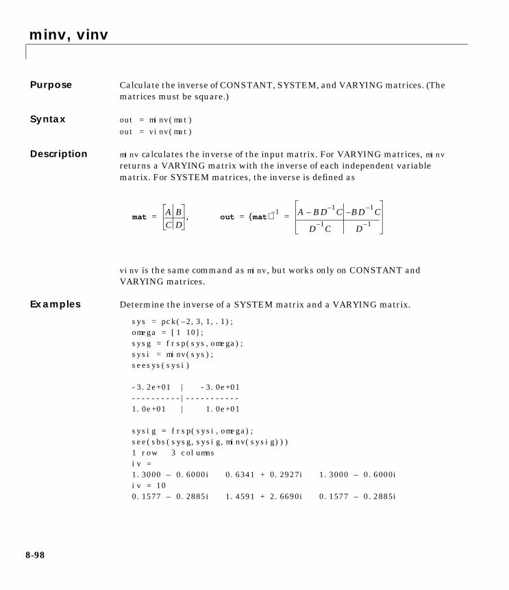
minv, vinv
8minv, vinvPurpose Calculate the inverse of CONSTANT, SYSTEM, and VARYING matrices. (Thematrices must be square.)
Syntax out = minv(mat) out = vinv(mat)
Description minv calculates the inverse of the input matrix. For VARYING matrices, minvreturns a VARYING matrix with the inverse of each independent variablematrix. For SYSTEM matrices, the inverse is defined as
vinv is the same command as minv, but works only on CONSTANT andVARYING matrices.
Examples Determine the inverse of a SYSTEM matrix and a VARYING matrix.
sys = pck(–2,3,1,.1); omega = [1 10]; sysg = frsp(sys,omega); sysi = minv(sys); seesys(sysi)
-3.2e+01 | -3.0e+01----------|-----------1.0e+01 | 1.0e+01
sysig = frsp(sysi,omega); see(sbs(sysg,sysig,minv(sysig)))1 row 3 columnsiv =1.3000 – 0.6000i 0.6341 + 0.2927i 1.3000 – 0.6000iiv = 100.1577 – 0.2885i 1.4591 + 2.6690i 0.1577 – 0.2885i
matA BC D
,= out mat( ) 1– A BD 1– C– BD 1– C–
D1–C D
1–= =
8-98

minv, vinv
Algorithm minv and vinv call the MATLAB inv command.
See Also inv, vdet
8-99

mmult
8mmultPurpose Multiply CONSTANT, SYSTEM, and VARYING matrices
Syntax out = mmult(mat1,mat2,,matN)
Description mmult allows the multiplication of matrices, mat1 and mat2 regardless of theirtype, provided their dimensions are compatible. CONSTANT, SYSTEM andVARYING matrices can be multiplied by one another based on the followingtable:
For compatibility, the number of columns of mat1 must equal the number ofrows of mat2. In the case of SYSTEM matrices, the number of inputs of mat1must equal the number of outputs of mat2. (An alternative term for themultiplication of two SYSTEM matrices is cascade.) Similarly restrictionsapply for VARYING matrices. Up to nine matrices of compatible dimension canbe multiplied via the same command by including them as input arguments.
Pictorial Representation of Function
mat2 CONSTANT SYSTEM VARYING
mat1
CONSTANT yes yes yes
SYSTEM yes yes no
VARYING yes no yes
8-100

mmult
Examples The multiplication (cascade) of two SYSTEM matrices is shown below.
seesys(p1)
–1.0e+01 | 1.0e+00----------|----------1.0e+01 | 1.0e+00
minfo(p1)system: 1 states 1 outputs 1 inputsseesys(p2)
–3.0e+00 | 2.0e+00----------|---------- 4.0e+00 | 1.0e-01
minfo(p2)system: 1 states 1 outputs 1 inputsout = mmult(p1,p2) seesys(out,%5.2g')
–10 4 | 0.1 0 -3 | 2---------|------ 10 0 | 0
Algorithm mmult uses the MATLAB “ *
” command when the multiplication does notinvolve two SYSTEM matrices. The equation for the multiplication of twosubsystems is given by
See Also *, abv, madd, mscl, msub
sys1A1 B1
C1 D1
,= sys2A2 B2
C2 D2
,=
mmult(sys1,sys2)→
A1 B1C2 B1D2
0 A2 B2
C1 D1C2 D1D2
=
8-101

mprintf
8mprintfPurpose Format output of matrix to screen
Syntax mprintf(matin,'format','end of line characters')
Description mprintf displays a matrix in formatted form. The optional 'format' specifiesthe format exactly as in the MATLAB function sprintf. If no 'format' isspecified the default is '%.1e'. This routine is primarily for use in seesys anddoes not work well for f format when the minimum field width is too small.There is no input checking, so you can wreak havoc if you use mprintfincorrectly. See sprintf for more details. The optional 'end of line characters' is exactly what it says. The default is the newline C escapesequence (\n). To get no newline at the end of each line usemprintf(matin,'format',[]).
Examples The mprintf command displays any type of matrix. An example of its use forSYSTEM and VARYING matrices follows:
mprintf(m)
1.7e+01 8.7e+00 –6.4e+00 –1.3e+015.9e–01 –1.4e+01 5.8e+00 –1.3e+011.8e+01 –7.0e+00 –3.6e+00 9.8e+002.6e+00 1.2e+01 –1.4e+00 –4.5e–01
mprintf(m,'%6.2f ')
16.96 8.72 –6.39 –13.490.59 –14.46 5.77 –12.7017.97 –7.01 –3.60 9.852.64 12.46 –1.36 –0.45
mprintf (m, '%3.f ')
17 9 –6 –13 1 –14 6 –1318 –7 –4 10 3 12 –1 –O
See Also fprintf, rifd, see, seesys, sprintf
8-102
msf, msfbatch
8msf, msfbatchPurpose Interactive D-scaling rational fit routine used in µ-synthesis
Syntax [dsysL,dsysR] = msf(Mg,bnds,dvec,sens,blk) [dsysL,dsysR] = msfbatch(Mg,bnds,dvec,sens,blk,maxord)
Description msf fits the block diagonal, frequency-dependent matrices DL(ω) and DR(ω)(contained in the VARYING matrix dvec, with block structure implied by theentries of blk) with rational, stable, minimum-phase and suchthat
msf returns the stable, minimum phase system matrices dsysL and dsysR.
NOTE: Typically, there is no need to call msf directly. The standard use of msf is a subroutine within µ-synthesis. The programs dkit and/or dkitgui arefully functional µ-synthesis routines.
Input arguments:
Mg is the frequency response upon which the µ calculation wasperformed.
bnds is the upper bound from the µ calculation.
dvec is a frequency varying vector containing the Ds (obtained frommu).
sens is the sensitivity of the upper bound in the µ calculation on theDs. The sensitivity sens is a frequency domain weight calculatedby mu.
blk is the uncertainty block structure. This should correspond withthe block strcucture used in the µ calculation (and produced bnds,dvec and sens).
DL s( ) DR s( )
maxσ DL ω( )M jω( )DR1– ω( )[ ] DLMDR
1–∞≈
8-103

msf, msfbatch
Output arguments:
msftbatch is a batch version of msf with no user interaction.
See Also dkit, dkitgui, fitmag, fitmaglp, fitsys, genphase, magfit
dsysL is the left (i.e., output) block diagonal scaling matrix. It is aSYSTEM matrix (it may be CONSTANT)
dsysR is the right (i.e., input) block diagonal scaling matrix. It is thesame type as dsysL
8-104

mscl, sclin, sclout
8mscl, sclin, scloutPurpose Scale CONSTANT, SYSTEM and VARYING matrices
Syntax matout = mscl(matin,fac); matout = sclin(matin,inputs,fac); matout = sclout(matin,outputs,fac);
Description The mscl command scales the individual elements of a CONSTANT orVARYING matrix by the scalar fac. mscl produces a CONSTANT (VARYING)matrix, matout, given matin is a CONSTANT (VARYING) matrix, and fac is ascalar. When the output matrix, matout, is VARYING, it has the sameindependent variable values as matin, and is equal to matin multiplied by thescalar value fac. If matin is a SYSTEM matrix, then mscl produces a SYSTEMmatrix, matout, in which the A and C matrices of matin are unchanged, and theB and D matrices have been scaled by fac. fac must be a scalar.
The command sclin scales the input channels to the matrix matin (which canbe a CONSTANT, SYSTEM or VARYING matrix) defined by the variableinputs. inputs is a vector of integers, which selects the inputs channels(columns) to be scaled by fac. The command sclout performs the similarscaling on the outputs (or rows). fac can be a scalar, single-input/single-output(SISO) SYSTEM or a VARYING, 1 × 1, matrix. If matin and fac are bothVARYING matrices, they must have the same independent variables to beused with sclin and sclout. The following options can be performed usingsclin and sclout:
• Scale select inputs and outputs of a SYSTEM or CONSTANT (matin) matrixby a scalar or a SISO SYSTEM (fac).
• Scale select inputs and outputs of a VARYING matrix by a scalar.
• Scale select inputs and outputs of a VARYING matrix by a VARYING(matin), 1 × 1, matrix (fac).
8-105

mscl, sclin, sclout
Examples mscl scales the three input, two output VARYING matrix, matin, by –2.5.
minfo(matin)varying– 2 pts2 rows3 colssee(matin)2 rows 3 columnsindep variable0.23 13 234 14 24indep variable0.34 14 245 15 25matout = mscl(matin,–2.5);see(matout)2 rows 3 columnsindep variable0.2–7.5000–32.5000–57.5000–10.0000–35.0000–60.0000indep variable0.3–10.0000–35.0000–60.0000–12.5000–37.5000–62.5000
8-106

mscl, sclin, sclout
Use the sclin command to scale the first input of a SYSTEM matrix by –3.
sys = pck(ones(3,3),2*ones(3,2),3*ones(1,3),4*ones(1,2));seesys(sys)
1.0e+00 1.0e+00 1.0e+00 | 2.0e+00 2.0e+001.0e+00 1.0e+00 1.0e+00 | 2.0e+00 2.0e+001.0e+00 1.0e+00 1.0e+00 | 2.0e+00 2.0e+00------------------------------------------------------3.0e+00 3.0e+00 3.0e+00 | 4.0e+00 4.0e+00
sysout = sclin(sys,1,–3);
seesys(sysout)
1.0e+00 1.0e+00 1.0e+00 | –6.0e+00 2.0e+001.0e+00 1.0e+00 1.0e+00 | –6.0e+00 2.0e+001.0e+00 1.0e+00 1.0e+00 | –6.0e+00 2.0e+00-------------------------------------------------------3.0e+00 3.0e+00 3.0e+00 | –1.2e+01 4.0e+00
The sclout command can be used to scale the first and third outputs of a SYSTEM matrix by the first order transfer function 10/(s + 10).
sys = sysrand(2,3,1);seesys(sys,'%11.2e)
2.19e–01 6.79e–01 | 9.35e–014.70e–02 6.79e–01 | 3.84e–01----------------------------------5.19e–01 5.35e–02 | 7.70e–038.31e–01 5.30e–01 | 3.83e–013.46e–02 6.71e–01 | 6.68e–02
8-107
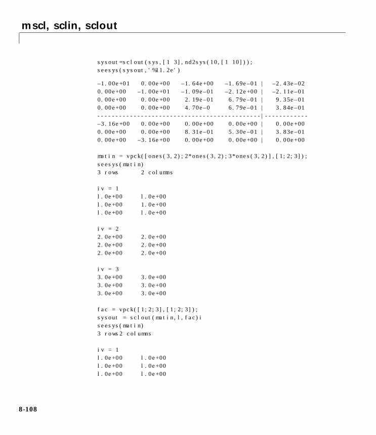
mscl, sclin, sclout
sysout=sclout(sys,[1 3],nd2sys(10,[1 10]));seesys(sysout,'%11.2e')
–1.00e+01 0.00e+00 –1.64e+00 –1.69e–01 | –2.43e–020.00e+00 –1.00e+01 –1.09e–01 –2.12e+00 | –2.11e–010.00e+00 0.00e+00 2.19e–01 6.79e–01 | 9.35e–010.00e+00 0.00e+00 4.70e–0 6.79e–01 | 3.84e–01---------------------------------------------|------------–3.16e+00 0.00e+00 0.00e+00 0.00e+00 | 0.00e+000.00e+00 0.00e+00 8.31e–01 5.30e–01 | 3.83e–010.00e+00 –3.16e+00 0.00e+00 0.00e+00 | 0.00e+00
matin = vpck([ones(3,2);2*ones(3,2);3*ones(3,2)],[1;2;3]);seesys(matin)3 rows 2 columns
iv = 1l.0e+00 l.0e+00l.0e+00 1.0e+00l.0e+00 l.0e+00
iv = 22.0e+00 2.0e+002.0e+00 2.0e+002.0e+00 2.0e+00
iv = 33.0e+00 3.0e+003.0e+00 3.0e+003.0e+00 3.0e+00
fac = vpck([1;2;3],[1;2;3]);sysout = sclout(matin,l,fac)iseesys(matin)3 rows2 columns
iv = 1l.0e+00 l.0e+00l.0e+00 l.0e+00l.0e+00 l.0e+00
8-108

mscl, sclin, sclout
iv = 24.0e+00 4.0e+002.0e+00 2.0e+002.0e+00 2.0e+00
iv = 39.0e+00 9.0e+003.0e+00 3.0e+003.0e+00 3.0e+00
See Also *, mmult, scliv, and sel
8-109

mu, muunwrap, randel, unwrapd, unwrapp
8mu, muunwrap, randel, unwrapd, unwrappPurpose Compute upper and lower bounds for the complex and mixed (real andcomplex) structured singular value (referred to as mixed µ) of a VARYING/CONSTANT matrix
Syntax [bnds,dvec,sens,pvec,gvec] = mu(matin,blk,options);[dl,dr,gl,gm,gr,pert] = muunwrap(dvec,gvec,pvec,blk);[dl,dr,gl,gm,gr] = muunwrap(dvec,gvec,blk);[dl,dr] = muunwrap(dvec,blk);pert = randel(blk,nrm,opt);[dl,dr] = unwrapd(dvec,blk);pert = unwrapp(pvec,blk);
The functions associated with mixed µ are:
mu general complex and mixed computation
muunwrap extract block-diagonal D- and G- scalings from row vectorscontaining the scalings
randel create random block structured matrix
unwrapd extract block-diagonal D-scalings from row vectorcontainingthe scalings
unwrapp extract block-diagonal perturbation from row vectorcontaining the perturbation
8-110

mu, muunwrap, randel, unwrapd, unwrapp
Description Input arguments:
matin A CONSTANT or VARYING matrix
blk An array that describes the perturbation block structure. Itssize is nblk × 2, where nblk is the total number of blocks inthe perturbation structure. The ith row of blk defines thedimensions of the ith perturbation block. If blk(i,:) = [–r 0], then the ith block is an r × r repeated, diagonal realscalar perturbation, while if blk(i,:) = [r 0], then the ithblock is an r × r repeated, diagonal complex scalarperturbation, and if is blk(i,:) = [r c], then the ith blockis an r × c complex full-block perturbation. If blk is omitted,the default is all 1 × 1 complex blocks, and results in anerror if matin is not square.
options An optional character string describing the desiredcomputations. It can consist of the following characters:'l' - compute lower bound using a power iteration't' - use more iterations in the lower bound'R' - start power iteration with RANDOM vectors'Rj' - restart lower bound j times with RANDOM vectorswhere j is an integer between 1 and 9'u' - compute upper bound using a balanced/LMI technique'c' - compute upper bound to greater accuracy'C''C' - compute tighest upper bound (may be slow)'f' - compute a fast but crude upper bound'r' - restart computation at EACH independent variable's' - suppress progress information'w' - suppress warnings'L' - compute only the lower bound'U' - compute only the upper bound
8-111

mu, muunwrap, randel, unwrapd, unwrapp
The default value of options is 'lu', meaning that a lower bound will becomputed using the power method, Young and Doyle 1990 and Packard et al.1988, and an upper bound will be computed, using the balanced/AMItechnique, Young et al., 1992, for computing the upper bound from Fan et al.,1991.
Output arguments:
[dl,dr,gl,gm,gr] = muunwrap(dvec,gvec,blk);
The upper bound in bnds for a matrix M is a number β > 0 such that there arescaling matrices Dl, Dr, Gl, Gm, Gr (see Young et al., 1992, for details) satisfying
sens is a row vector which contains the sensitivity of
with respect to the values in Dl (and Dr). It is calculated in an ad-hoc manner,and is mainly used when fitting frequency varying Ds with rational functionsvia the routines in dkit, dkitgui, and autodkit.
bnds A 1 × 2 vector. If matin is VARYING, so is bnds, whereas ifmatin is a CONSTANT matrix, then bnds is CONSTANT.The first column of bnds contains an upper bound to mixedµ of matin, and the second column contains a lower boundto mixed µ.
dvec and gvec Row vectors which contain the D and G scaling matricesthat have produced the upper bound in bnds. dvec and gvecare the same data type as bnds and are stored as vectors tosave memory. They can be unwrapped into the appropriateD and G matrices by using the command, muunwrap:
σ I Gl2
+( )14---– DlMDr
1–
β----------------------- jGm–
I Gr2
+( )14---–
1≤
σ DlMDr1–( )
8-112
mu, muunwrap, randel, unwrapd, unwrapp
pvec is a row vector containing a perturbation matrix that has the structuredefined by blk. As with dvec and gvec, pvec is the same data type as matin andis stored as a vector. It can be unwrapped into the actual perturbation with thecommand, unwrapp:
pert = unwrapp(pvec,blk);
After being unwrapped, the perturbation matrix pert satisfies threeconditions:
• It has the block structure defined by blk;
• The maximum singular value of pert is equal to the reciprocal of the lowerbound in bnds (when the lower bound is not zero);
• The matrix mmult(matin,pert) has an eigenvalue equal to 1 at eachindependent variable.
Examples Suppose sys is a system matrix with four inputs and four outputs, and that itis stable. sys_g is a frequency response of sys.
% ∆ is 4 1 × 1 perturbation blocksblk = ones(4,2);
8-113

mu, muunwrap, randel, unwrapd, unwrapp
% Calculate µ on frequency response[bnds,dvec,sens,pvec] = mu(sys_g,blk);
% Unwrap the D scaling matrices[dl,dr] = unwrapd(dvec,blk);
% Generate scaled matrixdmdi = mmult(dl,sys_g,minv(dr));
% Verify the upper boundvplot('liv,m',vnorm(dmdi),sel(bnds,1,1))
% Unwrap the perturbationactpert = unwrapp(pvec,blk);
% Check that perturbation is correct structuresee(xtracti(actpert,1))
% Check lower bound and perturbationvplot('liv,lm',sel(bnds,1,2),vnorm(actpert))
8-114

mu, muunwrap, randel, unwrapd, unwrapp
% Form M∆mdel = mmult(sys_g,actpert);
% Verify M∆ has an eigenvalue at 1veig(mdel)
Looking at the same frequency response sys_g with a mixed real/complex blockstructure:
% ∆ is 4 1 × 1 perturbation blocks
% with the first 2 real, and the last 2 complexblk = [–1 0; –1 0; 1 0; 1 0];
% Calculate mixed µ on frequency response[bnds,dvec,sens,pvec,gvec] = mu(sys_g,blk);
% Unwrap the D and G scaling matrices[dl,dr,gl,gm,gr] = muunwrap(dvec,gvec,blk);
% Generate scaled matrixdmd = mmult(dl,sys_g,minv(dr)); oobdmd = veval('*',dmd,minv(sel(bnds,1,1))); oobdmdjg = msub(oobdmd,mscl(gm,j)); scall = madd(eye(4),mmult(gl,gl)); scalr = madd(eye(4),mmult(gr,gr)); scall = veval(,scall,-0.25); scalr = veval(”,scalr,-0.25); scaledmat = mmult(scall,oobdmdjg,scalr);
% Verify the upper bound (scaledmat should have norm ≤1)vplot('liv,m',vnorm(scaledmat))
% Unwrap the perturbationpert = unwrapp(pvec,blk);
% Check that perturbation is correct structuresee(xtracti(pert,1))
% Check lower bound and perturbationvplot('liv,m',sel(bnds,1,2),minv(vnorm(pert)))
8-115

mu, muunwrap, randel, unwrapd, unwrapp
% Form M∆mdel = mmult(sys_g,pert);
% Verify M∆ has an eigenvalue at 1see(veig(mdel))
For more examples of computing bounds for µ, please refer to the“Computational Exercise with the mu Command” and “ComputationalExercise with the mu Command — Mixed Perturbations” sections in Chapter4 as well as the robust multivariable control design examples in Chapters 6and 7.
Algorithm Peter Young and Matt Newlin helped write the mu program and supportingroutines.
The lower-bound power algorithm is from Young and Doyle, 1990, and Packardet al. 1988.
The upper-bound is an implementation of the bound from Fan et al., 1991,and is described in detail in Young et al., 1992. In the upper boundcomputation, the matrix is first balanced using either a variation of Osborne’smethod (Osborne, 1960) generalized to handle repeated scalar and full blocks,or a Perron approach. This generates the standard upper bound for theassociated complex µ problem. The Perron eigenvector method is based on anidea of Safonov, (Safonov, 1982). It gives the exact computation of µ forpositive matrices with scalar blocks, but is comparable to Osborne on generalmatrices. Both the Perron and Osborne methods have been modified tohandle repeated scalar and full blocks. Perron is faster for small matrices buthas a growth rate of n3, compared with less than n2 for Osborne. This is partlydue to the MATLAB implementation, which greatly favors Perron. Thedefault is to use Perron for simple block structures and Osborne for morecomplicated block structures. A sequence of improvements to the upperbound is then made based on various equivalent forms of the upper bound. Anumber of descent techniques are used which exploit the structure of theproblem, concluding with general purpose AMI optimization (Boyd et al.),1993, to obtain the final answer.
8-116

mu, muunwrap, randel, unwrapd, unwrapp
Reference S. Boyd, and L. El Ghaoui, “Methods of centers for minimizing generalizedeigenvalues,” Linear Algebra and Its Applications, vol. 188–189, pp. 63–111,1993.
M. Fan, A. Tits, and J. Doyle, “Robustness in the presence of mixed parametricuncertainty and unmodeled dynamics,” IEEE Transactions on AutomaticControl, vol. AC–36, pp. 25–38, 1991.
E. Osborne, “On preconditioning of matrices,” Journal of Associated ComputerMachines, vol. 7, pp. 338–345, 1960.
A. Packard, M. Fan and J. Doyle, “A power method for the structured singularvalue,” Proc. of 1988 IEEE Conference on Control and Decision, pp. 2132–2137,December 1988.
M. Safonov, “Stability margins for diagonally perturbed multivariablefeedback systems,” IEEE Proc., vol. 129, Part D, pp. 251–256, 1982.
P. Young and J. Doyle, “Computation of with real and complex uncertainties,”Proceedings of the 29th IEEE Conference on Decision and Control, pp. 1230–1235, 1990.
P. Young, M. Newlin, and J. Doyle, “Practical computation of the mixedproblem,” Proceedings of the American Control Conference, pp. 2190–2194,June, 1992.
See Also blknorm, dypert, genmu, norm, vnorm, vrho, vsvd
8-117

musynfit, musynflp, muftbtch
8musynfit, musynflp, muftbtchPurpose Interactive D-scaling rational fit routines used in old µ-synthesis routines
Note: These routines are included only for backwards compatibility withversions 1.0 and 2.0. They will not be supported in future versions. Theyshould not be used by new users of the toolbox. All new routines should bebased on the new routine, msf, which is described on page ???.
Syntax [dsysL,dsysR] = musynfit(pre_dsysL,dvec,sens,blk,...nmeas,ncntrl,clpg,upbd,wt)
[dsysL,dsysR] = musynflp(pre_dsysL,dvec,sens,blk,...nmeas,ncntrl,clpg,upbd,wt)
[dsysL,dsysR] = muftbtch(pre_dsysL,dvec,sens,blk,... nmeas,ncntrl,dim)
Description musynfit fits the magnitude curve obtained by multiplying the old D frequencyresponse (from pre_dsysl) with the dvec data. musynfit returns stable,minimum phase system matrices dsysL and dsysR, which can be absorbed intothe original interconnection structure. Once absorbed, a H∞ design isperformed with hinfsyn completing another D–K iteration of µ-synthesis.
For the first µ-synthesis iteration, set the variable pre_dsysl to the stringfirst. In subsequent iterations, pre_dsysl should be the previous (left)rational D-scaling system matrix, dsysL. Essentially, the element-by-elementmagnitudes of the matricesmmult(unwrapd(dvec,blk),frsp(pre_dsysL,getiv(dvec))), andfrsp(dsysL,getiv(dvec)) are equal.
The (optional) variable clpg is the VARYING matrix that produced the dvec,sens, and upbd data output from µ. The fitting procedure is interactive(musynfit or musynflp), and fits (in magnitude) these scalings with rational,stable transfer function matrices, . After fitting the dvec data, plots of
and
D s( )
σ Df jω( ) clpg jω( ) Df1– jω( )⋅ ⋅( )
8-118

musynfit, musynflp, muftbtch
are shown in the lower graph window for comparison. At this point, you havethe option of refitting the D data. If clpg and upbd are not provided, the defaultis to plot the sens variable in the the lower graph.
Note: You are strongly discouraged from calling musynfit and musynflpdirectly and are encouraged to use dkit or dkitgui to perform µ-synthesiscalculations.
Input arguments:
pre_dsysl is set to the character string 'first' for the first iteration.As the iteration proceeds, it should be the previous dsysL.
sens is the sensitivity of the upper bound in the µ calculation onthe Ds. The sensitivity sens is a frequency domain weight,which is obtained from mu.
dvec is a frequency varying row vector containing the Ds (from mu).
blk is the block structure, same block structure used in mu.
nmeas is the number of measurements in control problem.
ncntrl is the number of controls in control problem.
clpg is the frequency response upon which the calculation wasperformed (optional).
upbd is the upper bound from the µ calculation (optional).
wt is a weight used to influence the frequency range in which thedata is to be fit more accurately (optional).
dim is the highest order fit to be used (only used in muftbtch).
σ D jω( ) clpg jω( ) D1–
jω( )⋅ ⋅( )
8-119

musynfit, musynflp, muftbtch
Output arguments:
For more detail about the role of hmax and htol, see the reference pages forfitmaglp and magfit. Reasonable choices are hmax = .26 and htol = .1.
The musynflp and musynfit commands provide the option of fitting thefrequency varying D-scale data by hand using the µ-Tools drawmag command.You can invoke this option with the string 'drawmag' in response to the prompt
ENTER ORDER OF CURVE FIT or 'drawmag'
The mouse is used in the plot window to identify the data to be fit with a stable,minimum-phase system. See the drawmag command for more information.
Examples musynfit is used within a D–K iteration (µ-synthesis) to fit the D-scales, whichare output from the mu command. The first step in the D–Kiteration is to designan H∞ control law. The closed-loop system is analyzed with mu based on theblock structure blk defined. The optimal D-scaling output from mu, which arereal coeeficients, are fit with real, rational, minimum-phase stable transferfunctions via musynfit. These fitted D-scales are wrapped back around theorginal interconnection structure P. After absorbing the D-scales, another D–Kiteration is performed, starting with the design of an H∞ control law for the
dsysL is the output (left) block diagonal, SYSTEM scaling.
dsysR is the input (right) block diagonal, SYSTEM scaling (needs tobe inverted before being absorbed into the interconnectionstructure).
musynflp has the same inputs and outputs and user interaction asmusynfit but uses a linear programing routine to do thefitting. muftbtch is a batch version of musynflp that has nouser interaction. The extra argument dim is a requiredargument of parameters for the linear program. dim has theform [hmax htol nmin nmax] where• hmax is a measure of the allowable error in the fit.
• htol is a measure of the accuracy with which the optimiza-tion is carried out.
• nmin and nmax are the minimum and maximum orders con-sidered in the problem
8-120

musynfit, musynflp, muftbtch
modified plant. This process usually continues until the value of µ doesn’tchange significantly between control design iterations.
This example is taken from the “HIMAT Robust Performance Design Example”section in Chapter 7. himat_ic contains the open-loop interconnectionstructure. It has one multiplicative input perturbation, which is two by two,and has two error signals, and two external disturbances. There are twomeasurements, and two control inputs to the system. The block structure forthe µ-analysis problem is given by blk=[2 2; 2 2].
First step in a D–K iteration is to design an H∞ controller and analyze theclosed loop system with µ.
mkhic omega = logspace(0,4,40); blk = [2 2; 2 2]; [k1,g1,gf1] = hinfsyn(himat_ic,2,2,0.8,6,0.05,2); g1_g = frsp(g1,omega); [bnds1,dvec1,sens1,rp1] = mu(g1_g,blk);
The D-scalings output from the µ-analysis problem needs to be fit with real,rational, stable, minimum-phase transfer functions. This is done withmusynfit. The first D-scale is fit with both a first and third-order transferfunction, with the third order transfer function selected.
8-121
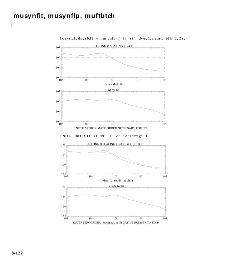
musynfit, musynflp, muftbtch
[dsysL1,dsysR1] = musynfit('first',dvec1,sens1,blk,2,2);
ENTER ORDER OF CURVE FIT or 'drawmag' 1
10-2
10-1
100
101
100 101 102 103 104
data and old fit
FITTING D SCALING #1 of 1
10-2
10-1
100
101
100 101 102 103 104
wt for fit
NOTE APPROXIMATE ORDER NECESSARY FOR FIT.....
10-2
10-1
100
101
100 101 102 103 104
1) data 2) newfit 3) oldfit
FITTING D SCALING #1 of 1, W/ORDER = 1
10-2
10-1
100
101
100 101 102 103 104
weight for fit
ENTER NEW ORDER, ’drawmag’, or NEGATIVE NUMBER TO STOP
8-122
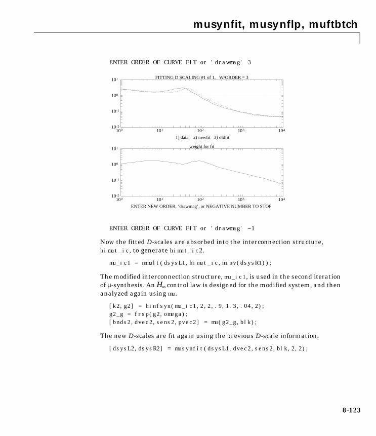
musynfit, musynflp, muftbtch
ENTER ORDER OF CURVE FIT or 'drawmag' 3
ENTER ORDER OF CURVE FIT or 'drawmag' –1
Now the fitted D-scales are absorbed into the interconnection structure,himat_ic, to generate himat_ic2.
mu_ic1 = mmult(dsysL1,himat_ic,minv(dsysR1));
The modified interconnection structure, mu_ic1, is used in the second iterationof µ-synthesis. An H∞ control law is designed for the modified system, and thenanalyzed again using mu.
[k2,g2] = hinfsyn(mu_ic1,2,2,.9,1.3,.04,2); g2_g = frsp(g2,omega); [bnds2,dvec2,sens2,pvec2] = mu(g2_g,blk);
The new D-scales are fit again using the previous D-scale information.
[dsysL2,dsysR2] = musynfit(dsysL1,dvec2,sens2,blk,2,2);
10-2
10-1
100
101
100 101 102 103 104
1) data 2) newfit 3) oldfit
FITTING D SCALING #1 of 1, W/ORDER = 3
10-2
10-1
100
101
100 101 102 103 104
weight for fit
ENTER NEW ORDER, ’drawmag’, or NEGATIVE NUMBER TO STOP
8-123

musynfit, musynflp, muftbtch
The graphs displayed with musynfit for this iteration are not included. Wrapthe new fitted D-scales around the original plant interconnection structure andstart D–K iteration again.
mu_ic2 = mmult(dsysL2,himat_ic,minv(dsysR2)); [k3,g3] = hinfsyn(mu_ic2,2,2,.9,1.3,.05,2);
musynfit can be called as before with the frequency response of the closed-loopsystem analyzed using mu, g1_g, and the mu upper bound, sel(bnds1,1,1)passed. The first D-scale is fit with both a first- and third-order transferfunction and the first order transfer function selected. As you can see from the
8-124

musynfit, musynflp, muftbtch
scaled upper bound plots (the lower graph), the first-order fit does a better jobminimizing the scaled upper bound.
[dsysL1,dsysR1] = ...musynfit('first',dvec1,sens1,blk,2,2,gl_g,sel(bnds1,1,1)
10-2
10-1
100
101
100 101 102 103 104
data and old fit
FITTING D SCALING #1 of 1
10-2
10-1
100
101
100 101 102 103 104
wt for fit
NOTE APPROXIMATE ORDER NECESSARY FOR FIT.....
8-125
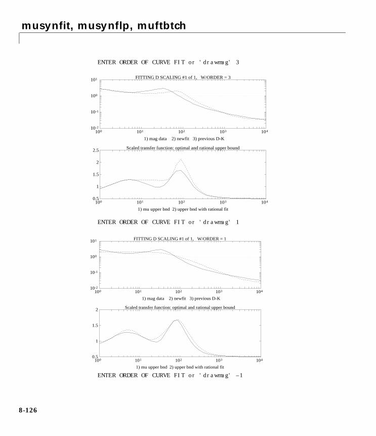
musynfit, musynflp, muftbtch
ENTER ORDER OF CURVE FIT or 'drawmag' 3
ENTER ORDER OF CURVE FIT or 'drawmag' 1
ENTER ORDER OF CURVE FIT or 'drawmag' –1
10-2
10-1
100
101
100 101 102 103 104
1) mag data 2) newfit 3) previous D-K
FITTING D SCALING #1 of 1, W/ORDER = 3
0.5
1
1.5
2
2.5
100 101 102 103 104
Scaled transfer function: optimal and rational upper bound
1) mu upper bnd 2) upper bnd with rational fit
10-2
10-1
100
101
100 101 102 103 104
1) mag data 2) newfit 3) previous D-K
FITTING D SCALING #1 of 1, W/ORDER = 1
0.5
1
1.5
2
100 101 102 103 104
Scaled transfer function: optimal and rational upper bound
1) mu upper bnd 2) upper bnd with rational fit
8-126
musynfit, musynflp, muftbtch
As before you would aborb the fitted D-scales into the interconnectionstructure, himat_ic, to generate himat_ic2.
Algorithm A frequency response is done on the previous rational D-scaling matrix. This ismultiplied by the current data in dvec, to produce the frequency varyingscaling that needs to be fit. The fit is only in magnitude, and the freedom in thephase allows the rational function to be defined as stable, and minimum phase.musynfit calls fitsys, which calls fitmag, flatten, and genphase. The curvefitting is done the fitsys command.
musynflp is an alternative program that uses linear programming to do the fit.musynflp fits the data very well within the frequency response window at theexpense of perhaps large variations outside the data window. This may lead toproblems in D–K iteration. muftbtch is a batch version of musynflp.
Reference J.C. Doyle, K. Lenz, and A.K. Packard, “Design examples using µ-synthesis:Space shuttle lateral axis FCS during reentry,” NATO ASI Series, Modelling,Robustness and Sensitivity Reduction in Control Systems, vol. F34 R.F. Curtin,Editor, Springer-Verlag, Berlin-Heidelberg, 1987.
See Also drawmag, fitmag, fitmaglp, fitsys, flatten, genphase, invfreqs, magfit, msf
8-127

ncfsyn, cf2sys, emargin
8ncfsyn, cf2sys, emarginPurpose ncfsyn synthesizes an H∞ controller to robustly stabilize a family of systemsgiven by a ball of uncertainty in the normalized coprime factors of the systemdescription
cf2sys calculates a SYSTEM/CONSTANT/VARYING matrix from a coprimefactorization.
emargin calculates the normalized coprime factor/gap metric robust stabilitymargin b(P,K) as defined in the “Loop Shaping Using H∞ Synthesis” section inChapter 3.
Syntax [sysk,emax,sysobs] = ncfsyn(sysgw,factor,opt) sysout = cf2sys(sysrcf) emarg = emargin(sys_g,sysw,tol)
Description A method of designing controllers is to use a combination of loop shaping androbust stabilization as proposed in McFarlane and Glover. The first step is todesign a pre- and post-compensator W1(s) and W2, so that the gain ofW2(s)P(s)W1(s) is sufficiently high at frequencies where good disturbanceattenuation is required and is sufficiently low at frequencies where good robuststability is required. The second step is to design a feedback controller, K∞, sothat
which will also give robust stability of the perturbed weighted plant
where NM–1 = W2PW1is a normalized coprime factorization satisfyingN(jw)*N(jw) + M(jw)*M(jw) = I. This stability margin is always less than 1 andgives a good indication of robust stability to a wide class of unstructuredperturbations, with values of ε > 0.2 – 0.3 generally satisfactory.
The closed-loop H∞-norm objective has the standard signal gain interpretation.Finally it can be shown that the controller, K∞, does not substantially affect the
1b W2PW1 K∞,( )----------------------------------------- :=
IK∞
I W2PW1 K∞,–( ) 1–W2PW1 I,[ ]
∞
ð1ε---
N ∆1+( ) M ∆2+( ) 1– for∆1
∆2 ∞
b W2PW1 K∞,( )<
8-128

ncfsyn, cf2sys, emargin
loop shape in frequencies where the gain of W2PW1 is either high or low, andwill guarantee satisfactory stability margins in the frequency region of gaincross-over. In the regulator set-up, the final controller to be implemented isW1K∞W2.
When the option 'ref' is specified, the controller includes an extra set ofreference inputs as proposed in Vinnicombe, 1993, and should be implemented
as u = sysk * where y = sysgw * u and r is a reference input. The
closed-loop response will then be y = Nr, where N is the numerator of anormalized right coprime factor of sysgw.
Input arguments
Output arguments
cf2sys creates a SYSTEM/CONSTANT/VARYING matrix from a coprimefactorization.
emargin calculates the normalized coprime factor/gap metric robust stabilitymargin b(P,K) as defined in the “Loop Shaping Using H∞ Synthesis” section in
sysgw the weighted system to be controlled
factor =1 implies that an optimal controller is required.>1 implies that a suboptimal controller is required achieving aperformance FACTOR less than optimal.
opt 'ref' the controller includes an extra set of reference input andshould be implemented as in Figure 3–12 on page 3-? (optional).
sysk H∞ loopshaping controller
emax Stability margin as an indication robustness to unstructuredperturbations. emax is always less than 1 and values of emaxgreater than 0.3 generally indicate good robustness margins.
sysobs H∞ loopshaping observer controller. This variable is created onlyif factor>1 and opt = 'ref'
yr
8-129

ncfsyn, cf2sys, emargin
Chapter 3. The default value for the tolerance tol supplied to the hinfnormcomputation is 0.001.
Algorithm See the McFarlane and Glover reference for details.
Reference McFarlane, D.C.and K. Glover, Robust Controller Design using NormalisedCoprime Factor Plant Descriptions, Springer Verlag, Lecture Notes in Controland Information Sciences, vol. 138, 1989.
McFarlane, D.C., and K. Glover, “A Loop Shaping Design Procedure usingSynthesis,” IEEE Transactions on Automatic Control, vol. 37, no. 6, pp. 759–769, June 1992.
Vinnicombe, G., “Measuring Robustness of Feedback Systems,” PhDdissertation, Department of Engineering, University of Cambridge, 1993.
See Also gap, hinfsyn, hinfnorm, nugap
8-130

nd2sys, zp2sys
8nd2sys, zp2sysPurpose Convert single-input/single-output (SISO) transfer functions to SYSTEMmatrices
Syntax sys = nd2sys(num,den,gain) sys = zp2sy(zeros,poles,gain)
Description nd2sys converts a numerator/denominator (num,den) SISO transfer functioninto a SYSTEM matrix, sys. This function uses the MATLAB command tf2ssfor the conversion. zp2sys converts zeros and poles of a SISO transfer functioninto a SYSTEM matrix, sys. This function uses the MATLAB command zp2ssto do the conversion. An optional argument gain can be supplied to scale thetransfer function. The default value of gain is 1. The output SYSTEM matrix,sys, is balanced with a call to the µ-Tools command sysbal prior to beingreturn if the real parts of the poles are all less than zero.
Examples Convert the single-input/single-output transfer function sys1 into a SYSTEMmatrix.
sys = nd2sys([4 5 1],[7 3 6 2 8]); minfo(sys)system:4 states1 outputs1 inputssee(sys)see (sys)
A matrix
sys 4s2
5s 1+ +
7s4
3s3
6s2
2s 8+ + + +-----------------------------------------------------------------=
8-131

nd2sys, zp2sys
B matrix1000
C matrix0 0.5714 0.7143 0.1429
D matrix0
Note: zp2sys requires the Signal Processing or Control Toolbox.
Algorithm nd2sys and zp2sys realize the transfer functions using the MATLABcommands tf2ss and zp2ss.
See Also pss2sys, pck, tf2ss
8-132

negangle
8neganglePurpose Calculate the angle of elements of a matrix, which is always between [–2π,0]
Syntax y = negangle(x)
Description negangle returns the phase angles, in radians, of a matrix with complex valuedelements. The returned value is always in the range 0 to –2π radians.
Examples a = [1+i,1–i];see(angle(a))0.7854–0.7854see(negangle(a))–5.4978–0.7854
See Also angle
8-133
pck, pss2sys, sys2pss, unpck
8pck, pss2sys, sys2pss, unpckPurpose Convert to and from CONSTANT and SYSTEM matrices
Syntax sys = pss2sys(mat,n) sys = pck(A,B,C,D) sys = pck(A,B,C) [A,B,C,D] = unpck(sys) mat = sys2pss(sys)
Description pss2sys translates a regular MATLAB matrix that is in packed form into aSYSTEM matrix. mat contains [A B; C D] which describes the individualcomponents of a SYSTEM matrix with n being the number of states (size of A).sys2pss returns the CONSTANT matrix, mat = [A B; C D], from the inputSYSTEM matrix sys.
pck takes consistent state-space data and forms a SYSTEM matrix with thedata structure defined. Consistent state-space data requires a square A matrix,a B matrix with the same number of rows as A, a C matrix with the samenumber of columns as A, and a D matrix with same number of columns of B androws of C. If the fourth input argument is omitted, then the Dmatrix is assumedto be identically zero, of appropriate dimensions. unpck is the inverse operationof pck, taking a SYSTEM matrix sys and converting it to A, B, C and DCONSTANT matrices.
Note that based on the data structure definition, a –Inf in the bottom rightcorner of a matrix denotes a SYSTEM matrix, with the top, right cornerelement of the matrix containing the number of states.
8-134

pck, pss2sys, sys2pss, unpck
Examples Create a SYSTEM matrix from MATLAB CONSTANT matrices via pss2sys.Define matrices A, B, C, and D as follows:
A = [–1 1; –1 –3]; B =[2 2; 2 2]i C = [3 3]; D = [4 4]mat = [A B; C D];sys = pss2sys(mat,2);minfo(mat)3 rows4 cols: regular MATLAB matrixmat =–1 1 2 2–1 –3 2 23 3 4 4minfo(sys)system: 2 states1 outputs2 inputsseesys(sys)
-1.0e+00 1.0e+00 | 2.0e+00 2.0e+00-1.0e+00 -3.0e+00 | 2.0e+00 2.0e+00----------------------|---------------------- 3.0e+00 3.0e+00 | 4.0e+00 4.0e+00
The same SYSTEM matrix can be constructed using the pck command.
sys = pck(A,B,C,D);minfo(sys)system: 2 states1 outputs2 inputsseesys(sys)
-1.0e+00 1.0e+00 | 2.0e+00 2.0e+00-1.0e+00 -3.0e+00 | 2.0e+00 2.0e+00----------------------|---------------------- 3.0e+00 3.0e+00 | 4.0e+00 4.0e+00
8-135

pck, pss2sys, sys2pss, unpck
Matrices A, B, C, and D can be constructed from sys using unpck.
[A,B,C,D] = unpck(sys); AA = –1 1–1 3BB = 2 22 2CC = 3 3DD = 4 4mat = sys2pss(sys); matmat =–1 12 2–1 –32 23 34 4
See Also minfo, nd2sys, vpck, vunpck, zp2sys
8-136
pkvnorm, vnorm
8pkvnorm, vnormPurpose Find the norm or peak norm of a VARYING matrix
Syntax [peak,indv,index] = pkvnorm(matin,p) out = (matin) out = (matin,p)
Description pkvnorm sweeps through the independent variable, calculating the norm ofeach matrix as specified by the input argument p, following the conventionfrom MATLAB’s norm command. The default for p is the largest singular valueof matin. The three output arguments all pertain to the peak and its location:peak value, peak, the independent variable’s value, indv, and the independentvariable’s index, index.
vnorm is a VARYING matrix version of MATLAB’s norm command. Theoperation of the norm command is identical to vnorm, except that vnorm alsoworks on CONSTANT and VARYING matrices, which produces a CONSTANTor VARYING output. vnorm returns the matrix out with its norm at eachindependent variable value.
Examples The two-input/two-output VARYING matrix matin has its independentvariable at 0.2 and 0.6. The vnorm command finds the largest singular value ofthe VARYING matrix at each value of the indepedent variable. pkvnormreturns the largest singular value of the VARYING matrix, its independentvariable value, and the index of the independent variable.
minfo(matin)varying:2 pts2 rows2 colssee(matin)2 rows2 columnsindep variable 0.2 1.0000 0 0 0.5000indep variable 0.6 4 0–5 1nrm = vnorm(matin,2); see(nrm)
8-137

pkvnorm, vnorm
1 row 1 columnindep variable 0.2 1indep variable 0.6 6.4510[peak,indv,index] = pkvnorm(matin); peakpeak = 6.4510indvindv = 0.6000indexindex == 2
Algorithm pkvnorm and vnorm call the MATLAB norm command.
See Also norm, vsvd
8-138

ric_eig
8ric_eigPurpose Solution of a Riccati equation via eigenvalue decomposition
Syntax [x1,x2,fail,reig_min] = ric_eig(ham,epp) x = x2/x1;
Description ric_eig (along with a call to x=x2/x1) solves the Riccati equation,
A′X + XA + XRX – Q = 0
with the constraint that the matrix A + RX has all of its eigenvalues in openleft-half plane. The data matrices A, R and Q come from the input Hamiltonianmatrix, ham, in the form
and it is assumed that R = R′, Q = Q′.
If ham has no jω axis eigenvalues, then there exists n × n matrices x1 and x2such that [x1; x2] spans the n-dimensional stable, invariant subspace of ham.If the matrix x1 is indeed invertible, then X := x2 * x1–1 satisfies the Riccatiequation and results in A + RX being stable. It is the only such matrix withthese properties.
ric_eig has internal error checking and returns a fail value of 1 if jω axiseigenvalues of ham are found. If this occurs, there is no n-dimensional, stableinvariant subspace, and hence no stabilizing Riccati solution. An eigenvalue isconsidered to be purely imaginary if the magnitude of the real part is less thanepp. The minimum real part of the eigenvalues is returned in reig_min. epp isan optional argument and its default value is 1e – 10.
Note: When a Hamiltonian has repeated eigenvalues, solving the Riccatiequation via the eigenvalue method may have problems. This is due to theMATLAB command eig incorrectly selecting the eigenvectors associated withthe repeated roots.
hamA RQ A ′–
=
8-139

ric_eig
Algorithm Under the assumption that the Hamiltonian matrix has a full set ofeigenvectors, the stable-invariant subspace is spanned by the eigenvectorsassociated with the stable eigenvalues. Hence, an eigenvalue-eigenvectordecomposition can obtain the stable invariant subspace of the Hamiltonianmatrix, ham. Assuming there are no jω axis eigenvalues, and that there is a fullset of eigenvectors, the two components, x1 and x2, can be generated bychoosing the eigenvectors associated with the stable eigenvalues. The ric_eigsubroutine operates on the assumption that the Jordan form of theHamiltonian is diagonal, and returns the stable invariant subspace, asspanned by the eigenvectors, in the two block form described above.
See Also eig, h2syn, hinfsyn, hinffi, ric_schr
8-140

ric_schr
8ric_schrPurpose Solve a Riccati equation via Schur decomposition
Syntax [x1,x2,fail,reig_min] = ric_schr(ham,epp) x = x2/x1
Description ric_schr (along with a call to x=x2/x1) solves the Riccati equation,
A′X + XA + XRX – Q = 0
such that A + RX is stable. A real Schur decomposition can obtain the stableinvariant subspace of the Hamiltonian matrix, ham. The data matrices A, R,and Q come from the input Hamiltonian matrix in the form
and it is assumed that and it is assumed that R = R′, Q = Q′.
If ham has no jω axis eigenvalues, then there exists n × n matrices x1 and x2such that [x1; x2] spans the n-dimensional stable, invariant subspace of ham.If x1 is invertible, then X := x2 * x1–1 satisfies the Riccati equation andresults in A + RX being stable. The output flag fail is nominally 0. If thereare jω-axis eigenvalues, fail is set to 1. If there are an unequal number ofpositive and negative eigenvalues, fail is set to 2, and if both conditionsoccur, fail = 3.
Algorithm ric_schr calls csord to produce an ordered complex Schur form, which isconverted to a real Schur form, and yields a stable, invariant subspace of theHamiltonian. The csord command orders the solution with negative realeigenvalues in the top half of the matrix and the positive real eigenvalues onthe bottom, and returns the stable solution. The input matrix is assumed to bea Hamiltonian matrix of size 2n with n stable eigenvalues and n unstableeigenvalues. The minimum real part of the eigenvalues is output to reig_min.epp is an optional argument and its default value is 1e–10.
See Also csord, h2syn, hinfsyn, hinffi, ric_eig, schur
hamA RQ A ′–
=
8-141

rifd
8rifdPurpose Display the real, imaginary, frequency and damping ratios of a CONSTANTinput vector
Syntax rifd(vec)
Description rifd displays the real, imaginary, frequency, and damping ratios of aCONSTANT input vector. The ith frequency is given by the
and its damping ratio is defined as real(sys(i))/ω(i).
Examples Display the poles of the SYSTEM matrix, sys.
sys = pck(rand(4,4),rand(4,2),rand(1,4)); rifd(spoles(sys))
real imaginary frequency damping–7.6287e–02 0.0000e+00 7.6287e–02 l.0000e+00 1.0820e–01 –4.6815e–01 4.8049e–01 –2.2519e–01 1.0820e–01 4.6815e–01 4.8049e–01 –2.2519e–01 1.4095e+00 0.0000e+00 1.4095e+00 –l.0000e+00
See Also eig, imag, spoles, real
real(sys(i))2
imag(sys(i)2+( )
12---
8-142

samhld
8samhldPurpose Create a sample-hold approximation of a continuous system
Syntax discout = samhld(sys,T)
Description samhld applies a sample-hold to the input of the continuous-time systems sys,and samples the output, to produce a discrete-time system, discout. Thesampling time is the same at the input and output, and is specified by T.
Examples Construct the system sys via the nd2sys command and verify that all of itspoles are in the closed left-half plane. Perform a sample hold of the system fora 200 Hz sample rate. All the poles for the discretized system, discout, arewithin the unit disk.
sys = nd2sys([1 2 4 5],[2 7 9 2]); spoles(sys)
–1.6114 + 1.0049i–1.6114 – 1.0049i–0.2773discout = samhld (sys ,1 / 2 0 0)seesys (discout, '%8 .4f ')
0.9826 -0.0223 -0.0050 | 0.0050o.0050 0.9999 -0.0000 | 0.00000.0000 0.0050 1.0000 | 0.0000-----------------------------|----------0.7500 -0.2500 2.0000 | 0.5000
spoles(discout)
0.9920 + 0.0050i0.9920 – 0.0050i0.9986
Algorithm Suppose that the continuous-time system has state-space representation
sys A BC D
.=
8-143

samhld
If u(t) is held constant over the interval [kT,(k + 1)T], then over that interval,the state evolution is governed by the differential equation
which captures the behavior of the continuous-time system, over one sampleperiod, while the input u(t) is held constant.
Let . Define as . Then W
appears as
Define Adisc := W11, and Bdisc := W12, and define the discretized system as
See Also exp, expm, tustin
x·
u·A B
0nu n× 0nu n×
xu
, x kT( )u kT( )
xk
uk
,= =
A :=A B
0nu n× 0nu n×W R
n nu+( ) n nu+( )×∈ W := eAT
WW11 W12
0 I=
discoutAdisc Bdisc
C D=
8-144

scliv
8sclivPurpose Scale the independent variable values of a VARYING matrix with an affinetransformation
Syntax vout = scliv(vin,factor,offset)
Description scliv scales the independent variable of a VARYING matrix in the followingmanner. Let indvi and newindvi denote the independent variable’s ith value,before and after applying scliv. Then, for each i, they are related as
newindvi = (factor × indvi) + offset
The default value for offset is zero.
Examples Scale the independent value of vin by a factor of 3 and offset it from its originalvalue by 0.5.
seeiv(vin)l.000e+002.000e+003.000e+00 4.000e+00 5.000e+00vout = scliv(vin,3,0.5)seeiv(vout)3.500e+006.500e+009.500e+00 1.250e+01 1.550e+01
See Also getiv, seeiv
8-145

sdhfnorm
8sdhfnormPurpose sdhfnorm calculates the induced norm of a sampled-data system
Syntax [gaml,gamu]=sdhfsyn(p,k,h,delay,tol)
Description sdhfnorm is concerned with the control of a continuous-time system by adiscrete-time controller. The continuous-time interconnection structurestructure, p of type SYSTEM, has state-space realization partitioned asfollows:
where the continuous-time disturbance inputs enter through B1, the outputsfrom the controller are held constant between sampling instants and enterthrough B2, the continuous-time errors to be kept small correspond to the C1partition, and the output measurements that are sampled by the controllercorrespond to the C2 partition. B2 has column size (ncon) and C2 has row size(nmeas). Note that the D matrix is assumed to be zero.
sdhfnorm calculates the maximum gain from the L2 norm of the disturbanceinputs to the L2 norm of the error outputs.
Input arguments:
Output arguments:
p SYSTEM interconnection structure matrix, (continuous-time)
k discrete-time controller
h sampling period
delay number of samples computational delay (default = 0)(integer ≥ 0 with default =0)
tol required relative accuracy
gaml lower bound on the norm
gamu upper bound on the norm
p
A B1 B2
C1 0 0
C2 0 0
=
8-146

sdhfnorm
Examples An illustrative example is given in the “Discrete-time and Sampled-data H∞Control” section in Chapter 3.
Algorithm sdhfnorm uses variations of the formulae described in the Bamieh and Pearsonpaper to obtain an equivalent discrete-time system. (These variations are doneto improve the numerical conditioning of the algorithms.) A preliminary step isto determine whether the norm of the continuous-time system over onesampling period without control is less than the given γ-value. This requires asearch and is, computationally, a relatively expensive step.
Subroutines called. dhfsyn, ham2schr, and compnorm
Reference Bamieh, B.A., and J.B. Pearson, “A General Framework for Linear PeriodicSystems with Applications to Sampled-Data Control,” IEEE Transactions onAutomatic Control, vol. AC–37, pp. 418-–435, 1992.
See Also dhfsyn, hinfsyne, hinffi, hinfnorm, hinfsyn, h2syn, h2norm, ric_eig, ric_schr
8-147

sdhfsyn
8sdhfsynPurpose sdhfsyn computes an H∞ controller for a sampled-data SYSTEMinterconnection matrix
Syntax [k,gfin] = sdhfsyn(p,nmeas,ncon,gmin,gmax,tol,h,... delay,ricmethd,epr,epp)
Description sdhfsyn is concerned with the control of a continuous-time system by adiscrete-time controller. The continuous-time interconnection structurestructure, p of type SYSTEM, has state-space realization partitioned as follows
where the continuous-time disturbance inputs enter through B1, the outputsfrom the controller are held constant between sampling instants and enterthrough B2, the continuous-time errors to be kept small correspond to the C1partition, and the output measurements that are sampled by the controllercorrespond to the C2 partition. B2 has column size (ncon) and C2 has row size(nmeas). Note that the D matrix is assumed to be zero.
sdhfsyn synthesizes a discrete-time controller to achieve a given norm (ifpossible) or find the minimum possible norm to within some tolerance.
sdhfsyn provides a γ iteration using the bisection method. Given a high and lowvalue of γ, gmax and gmin, the bisection method is used to iterate on the valueof γ in an effort to approach the optimal H∞ control design. If gmax = gmin, onlyone γ value is tested. The stopping criteria for the bisection algorithm requiresthe relative difference between the last γ value that failed and the last γ valuethat passed be less than tol. You can select either the eigenvalue or Schurmethod for solution of the Riccati equations with and without balancing. Theeigenvalue method is faster but can have numerical problems, while the Schurmethod is slower but generally more reliable.
The algorithm employed calculates an equivalent purely discrete-time problemfor each value of γ and then calls dhfsyn with γ = 1. The screen printing is thenderived from the tests performed by dhfsyn.
p
A B1 B2
C1 0 0
C2 0 0
=
8-148
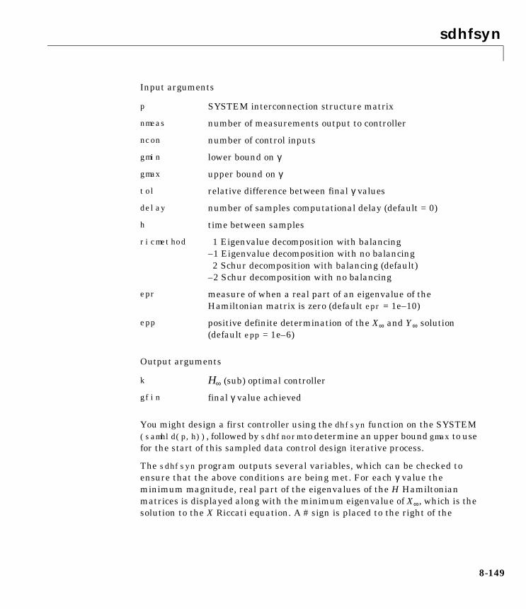
sdhfsyn
Input arguments
Output arguments
You might design a first controller using the dhfsyn function on the SYSTEM(samhld(p,h)), followed by sdhfnorm to determine an upper bound gmax to usefor the start of this sampled data control design iterative process.
The sdhfsyn program outputs several variables, which can be checked toensure that the above conditions are being met. For each γ value theminimum magnitude, real part of the eigenvalues of the H Hamiltonianmatrices is displayed along with the minimum eigenvalue of X∞, which is thesolution to the X Riccati equation. A # sign is placed to the right of the
p SYSTEM interconnection structure matrix
nmeas number of measurements output to controller
ncon number of control inputs
gmin lower bound on γ
gmax upper bound on γ
tol relative difference between final γ values
delay number of samples computational delay (default = 0)
h time between samples
ricmethod 1 Eigenvalue decomposition with balancing–1 Eigenvalue decomposition with no balancing
2 Schur decomposition with balancing (default)–2 Schur decomposition with no balancing
epr measure of when a real part of an eigenvalue of theHamiltonian matrix is zero (default epr = 1e–10)
epp positive definite determination of the X∞ and Y∞ solution(default epp = 1e–6)
k H∞ (sub) optimal controller
gfin final γ value achieved
8-149

sdhfsyn
condition that failed in the printout. This additional information can aid youin the control design process.
Examples An illustrative example is given in the “Discrete-time and Sampled-data H∞Control” section in Chapter 3.
Algorithm sdhfsyn uses variations of the formulae described in the Bamieh and Pearsonpaper to obtain an equivalent discrete-time system. (These variations are doneto improve the numerical conditioning of the algorithms.) A preliminary step isto determine whether the norm of the continuous-time system over onesampling period without control is less than the given γ-value, this requires asearch and is computationally a relatively expensive step.
Subroutines called. dhfsyn, ham2schr, compnorm
Reference Bamieh, B.A., and J.B. Pearson, “A General Framework for Linear PeriodicSystems with Applications to Sampled-Data Control,” IEEE Transactions onAutomatic Control, vol. AC–37, pp. 418–435, 1992.
See Also dhfsyn, hinfsyne, hinffi, hinfnorm, hinfsyn, h2syn, h2norm, ric_eig,ric_schr
8-150

see, seeiv
8see, seeivPurpose Display a SYSTEM or VARYING matrix
Syntax see(mat,iv_low,iv_high) see(matin) seeiv(mat)
Description see displays the A, B, C, and D matrices of matin for a SYSTEM matrix or theindependent variable and the matrix at that variable if matin is a VARYINGmatrix. iv_low and iv_high are the optional range of the independent variablesto be displayed. see displays the matrix itself if the input is CONSTANT.
seeiv displays only the independent variable of the input VARYING matrixmat. An error message is displayed if the input matrix is not a VARYINGmatrix.
Examples The see command displays any type of matrix. An example of its use forSYSTEM and VARYING matrices follows:
see(sys)A matrix1 11 1press any key to move to B matrixB matrix2 22 2press any key to move to C matrixC matrix3 3press any key to move to D matrixD matrix4 4sysg = frsp(sys,[0.4 0.9]);see(sysg)1 row2 columnsiv = 0.4–1.7692 – 1.1538i–1.7692 – 1.1538iiv = 0.9–0.9896 – 2.2453i–0.9896 – 2.2453i
See Also getiv, mprintf, rifd, seesys, sortiv
8-151
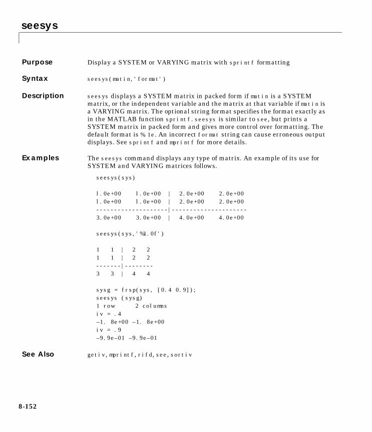
seesys
8seesysPurpose Display a SYSTEM or VARYING matrix with sprintf formatting
Syntax seesys(matin,'format')
Description seesys displays a SYSTEM matrix in packed form if matin is a SYSTEMmatrix, or the independent variable and the matrix at that variable if matin isa VARYING matrix. The optional string format specifies the format exactly asin the MATLAB function sprintf. seesys is similar to see, but prints aSYSTEM matrix in packed form and gives more control over formatting. Thedefault format is %.1e. An incorrect format string can cause erroneous outputdisplays. See sprintf and mprintf for more details.
Examples The seesys command displays any type of matrix. An example of its use forSYSTEM and VARYING matrices follows.
seesys(sys)
l.0e+00 l.0e+00 | 2.0e+00 2.0e+00l.0e+00 l.0e+00 | 2.0e+00 2.0e+00--------------------|---------------------3.0e+00 3.0e+00 | 4.0e+00 4.0e+00
seesys(sys,'%1.0f')
1 1 | 2 21 1 | 2 2-------|--------3 3 | 4 4
sysg = frsp(sys, [0.4 0.9]);seesys (sysg)1 row 2 columnsiv = .4–1. 8e+00 –1. 8e+00iv = .9–9.9e–01 –9.9e–01
See Also getiv, mprintf, rifd, see, sortiv
8-152

sel, reordsys
8sel, reordsysPurpose Select rows/outputs and columns/inputs from a CONSTANT, SYSTEM orVARYING matrix or reorder the SYSTEM states
Syntax out = sel(mat,rows,cols) out = sel(sys,outputs,inputs) sysout = reordsys(sys,index)
Description sel selects desired rows and columns from a CONSTANT/VARYING matrix,or outputs and inputs from a SYSTEM matrix. For CONSTANT and VARYINGmatrices, the rows and cols input arguments are row vectors with the desiredrows/columns of mat specified. For SYSTEM matrices, outputs and inputs arerow vectors with the desired inputs/outputs specified. Use the string ':' tospecify all rows (inputs) and/or columns (outputs).
reordsys reorders the states of SYSTEM matrix sys as defined by the vectorof position variables, index. The index variable is restricted to be the samelength as the number of states of sys. This command can be used in conjunctionwith strans and sresid to reduce the states of a SYSTEM matrix.
Examples You can use the sel command with any matrix type. First, construct anddisplay a one state, two output, three input SYSTEM matrix.
minfo(sys)system:1 states2 outputs3 inputsseesys(sys)
1.0e+00 | 2.0e+00 3.0e+00 4.0e+00---------|------------------------------5.0e+00 | 6.0e+00 7.0e+00 8.0e+009.0e+00 | 1.0e+01 1.1e+01 1.2e+01
Reorder the outputs of sys to be output 2, 1 and repeat output 2; also reorderthe inputs to be input 3, 1 and 2.
sys2 = sel(sys,[2 1 2],[3 1 2]); minfo(sys2)system:1 states3 outputs3 inputs
8-153

sel, reordsys
seesys(sys2) 1.0e+00 | 4.0e+00 2.0e+00 3.0e+00---------|------------------------------9.0e+00 | 1.2e+01 1.0e+01 1.1e+015.0e+00 | 8.0e+00 6.0e+00 7.0e+009.0e+00 | 1.2e+01 1.0e+01 1.1e+01
The same manipulations can be done on a VARYING matrix.
sysg =frsp(sys,logspace(–1,0,2)); see(sysg)2 rows3 columnsindep variable 0.1
–3.9010 – 0.9901i –7.8515 – 1.4851i –11.8020 – 1.9802i–7.8218 – 1.7822i –15.7327 – 2.6733i –23.6436 – 3.5644i
indep variable 1
1.0000 – 5.0000i –0.5000 – 7.5000i –2.0000 – 10.0000i1.0000 – 9.0000i –2.5000 – 13.5000i –6.0000 – 18.0000i
Select the second and first outputs and the third and second inputs and displaythem.
part = sel(sysg,[2 1],[3 2]); see(part)2 rows2 columnsindep variable 0.1
–23.6436 – 3.5644i –15.7327 – 2.6733i–11.8020 – 1.9802i –7.8515 – 1.4851i
indep variable 1
–6.0000 – 18.0000i –2.5000 – 13.5000i–2.0000 – 10.0000i –0.5000 – 7.5000i
8-154
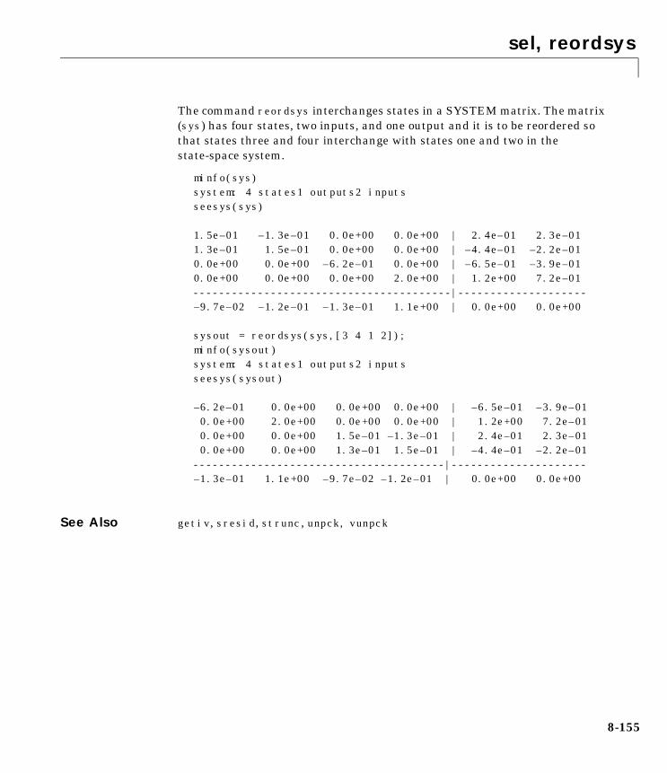
sel, reordsys
The command reordsys interchanges states in a SYSTEM matrix. The matrix(sys) has four states, two inputs, and one output and it is to be reordered sothat states three and four interchange with states one and two in thestate-space system.
minfo(sys)system: 4 states1 outputs2 inputsseesys(sys)
1.5e–01 –1.3e–01 0.0e+00 0.0e+00 | 2.4e–01 2.3e–011.3e–01 1.5e–01 0.0e+00 0.0e+00 | –4.4e–01 –2.2e–010.0e+00 0.0e+00 –6.2e–01 0.0e+00 | –6.5e–01 –3.9e–010.0e+00 0.0e+00 0.0e+00 2.0e+00 | 1.2e+00 7.2e–01----------------------------------------|--------------------–9.7e–02 –1.2e–01 –1.3e–01 1.1e+00 | 0.0e+00 0.0e+00
sysout = reordsys(sys,[3 4 1 2]);minfo(sysout)system: 4 states1 outputs2 inputsseesys(sysout)
–6.2e–01 0.0e+00 0.0e+00 0.0e+00 | –6.5e–01 –3.9e–01 0.0e+00 2.0e+00 0.0e+00 0.0e+00 | 1.2e+00 7.2e–01 0.0e+00 0.0e+00 1.5e–01 –1.3e–01 | 2.4e–01 2.3e–01 0.0e+00 0.0e+00 1.3e–01 1.5e–01 | –4.4e–01 –2.2e–01---------------------------------------|---------------------–1.3e–01 1.1e+00 –9.7e–02 –1.2e–01 | 0.0e+00 0.0e+00
See Also getiv, sresid, strunc, unpck, vunpck
8-155
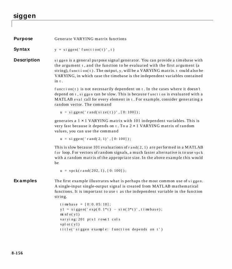
siggen
8siggenPurpose Generate VARYING matrix functions
Syntax y = siggen('function(t)',t)
Description siggen is a general purpose signal generator. You can provide a timebase withthe argument t, and the function to be evaluated with the first argument (astring), function(t). The output, y, will be a VARYING matrix. t could also beVARYING, in which case the timebase is the independent variables containedin t.
function(t) is not necessarily dependent on t. In the cases where it doesn’tdepend on t, siggen can be slow. This is because function is evaluated with aMATLAB eval call for every element in t. For example, consider generating arandom vector. The command
u = siggen('rand(size(t))',[0:100]);
generates a 1 × 1 VARYING matrix with 101 independent variables. This isvery fast because it depends on t. To a 2 × 1 VARYING matrix of randomvalues, you can use the command
u = siggen('rand(2,1)',[0:100]);
This is slow because 101 evaluations of rand(2,1) are performed in a MATLABfor loop. For vectors of random signals, a much faster alternative is to use vpckwith a random matrix of the appropriate size. In the above example this wouldbe
u = vpck(rand(202,1),[0:100]);
Examples The first example illustrates what is perhaps the most common use of siggen.A single-input single-output signal is created from MATLAB mathematicalfunctions. It is important to use t as the independent variable in the functionstring.
timebase = [0:0.05:10]; y1 = siggen('exp(0.1*t) – sin(3*t)',timebase); minfo(y1)varying:201 pts1 rows1 colsvplot(y1) title('siggen example: function depends on t')
8-156

siggen
The second example illustrates that the second argument can make use of theindependent values of a VARYING matrix. Note also that the specified functionis independent of t, and is executed at each instance of t. This example isincluded to illustrate that the function string need not depend on t. In practicethe string rand(size(t)) is orders of magnitude faster than rand.
y2 = siggen('rand',y1); minfo(y2)varying:201 pts1 rows1 colsvplot(y2) title('siggen example: function independent of t')
0
0.5
1
1.5
2
2.5
3
3.5
4
0 1 2 3 4 5 6 7 8 9 10
Siggen example: function depends on t
8-157

siggen
The use of siggen is not restricted to single-input, single-output signals. Thefollowing example creates a 2 × 2 VARYING matrix. In this example the matrixelements are all functions of t and the results plotted in the figure. They couldequally well have all been independent of t, for example 'rand(3,2)' could bethe function string. (Note that they must all be one type or the other (thisrestriction does not apply if t is a single number).
func = '[t/max(t) 2*cos(3*t+0.2); 2+0.1*sin(2*t) '; func = [func ' sqrt(t)+0.3*rand(size(t))]']; y3 = siggen(func,timebase); minfo(y3)varying:201 pts2 rows2 colsvplot(y3) title('Siggen example: 2 x 2 varying matrix')
0
0.1
0.2
0.3
0.4
0.5
0.6
0.7
0.8
0.9
1
0 1 2 3 4 5 6 7 8 9 10
Siggen example: function independent of t
8-158

siggen
siggen cannot generate stair-step signals with user-specified values. You cando this however (for single-input/single-output signals) using the commandvpck or the µ-Tools commmand step_tr. Vectors of signals can be created withvpck and abv. The following example demonstrates the use of vpck. vinterp isused to plot a meaningful representation of the signal.
y4 = vpck([0:10]',[0:2:20]'); minfo(y4)varying:11 pts1 rows1 colsvplot(vinterp(y4,0.1)) title('Siggen example: step function')
-2
-1
0
1
2
3
4
0 1 2 3 4 5 6 7 8 9 10
Siggen example: 2 x 2 varying matrix
8-159
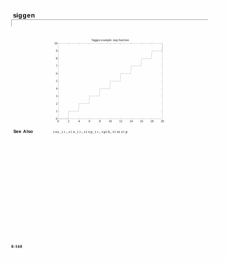
siggen
See Also cos_tr, sin_tr, step_tr, vpck, vinterp
0
1
2
3
4
5
6
7
8
9
10
0 2 4 6 8 10 12 14 16 18 20
Siggen example: step function
8-160
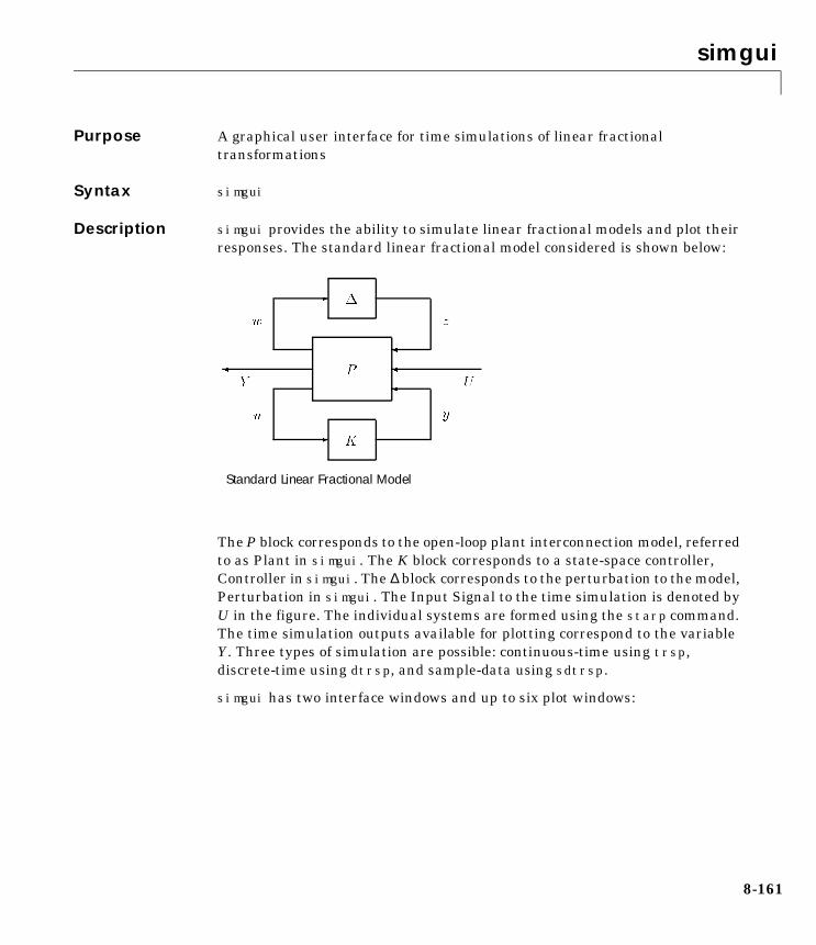
simgui
8simguiPurpose A graphical user interface for time simulations of linear fractionaltransformations
Syntax simgui
Description simgui provides the ability to simulate linear fractional models and plot theirresponses. The standard linear fractional model considered is shown below:
The P block corresponds to the open-loop plant interconnection model, referredto as Plant in simgui. The K block corresponds to a state-space controller,Controller in simgui. The ∆ block corresponds to the perturbation to the model,Perturbation in simgui. The Input Signal to the time simulation is denoted byU in the figure. The individual systems are formed using the starp command.The time simulation outputs available for plotting correspond to the variableY. Three types of simulation are possible: continuous-time using trsp,discrete-time using dtrsp, and sample-data using sdtrsp.
simgui has two interface windows and up to six plot windows:
Standard Linear Fractional Model
8-161

simgui
• Main Simulation window, which is the main interface for the user.
• Parameter window, which is used to modify properties of the timesimulation, such as the final time, integration step size, initial conditions,and which variables are automatically exported to the workspace.
• Plot windows, where the plots of time responses are displayed. You can openup to six of these windows.
A detailed description of the use and application of simgui is provided in the“LFT Time Simulation User Interface Tool: simgui” section in Chapter 6.
Examples An example of using simgui for simulation of a linear fractionaltransformation is shown in the “LFT Time Simulation User Interface Tool:simgui” section in Chapter 6.
See Also dtrsp, sdtrsp, starp, trsp, vplot
8-162

spoles
8spolesPurpose Calculate the eigenvalues of a SYSTEM A matrix
Syntax out = spoles(sys)
Description spoles returns the eigenvalues of the A matrix from the SYSTEM matrix sys.
Examples Find the poles of the two input, one output, three state SYSTEM matrx sys.
A = [1 1 1; 3 1 1; 1 1 –2]; B = 2*ones(3,2); C = 3*ones(1,3); D = 4*ones(1,2); sys = pck(A,B,C,D); minfo(sys)system: 3 states1 outputs2 inputsspoles(sys)3.1474–0.8186–2.3289eig(A)ans =3.1474–0.8186–2.3289
Algorithm spoles uses the MATLAB command schur to find the eigenvalues of theSYSTEM A matrix. This is a more numerically reliable method than using theeig function.
See Also eig, rifd, schur, szeros
8-163

srelbal, sfrwtbal, sfrwtbld, sncfbal, sdecomp
8srelbal, sfrwtbal, sfrwtbld, sncfbal, sdecompPurpose srelbal calculates the stochastically balanced realization of a SYSTEMmatrix, sfrwtbal, the frequency weighted balanced realization for performingrelative error, and sfrwtbld, the frequency weighted model order reduction.sncfbal calculates the normalized coprime factorizations. sdecomp decomposesa SYSTEM matrix as the sum of stable and unstable systems.
Syntax [sysb,relsv,sysfact] = srelbal(sys,tol) [sys1,sig1] = sfrwtbal(sys,wt1,wt2) syshat = sfrwtbld(sys1hat,wt1,wt2)[sysnlcf,signcf,sysnrcf] = sncfbal(sys,tol) [sysst,sysun] = sdecomp(sys,bord,fl)
Description srelbal performs a stochastically balanced realization of the input SYSTEMmatrix. sys must be stable and be of full column rank at infinite frequency, butnot necessarily square or minimum phase. Difficulties may occur if sys haszeros on the imaginary axis. sysb will have the same transfer function as sys,and sysfact gives the stable minimum phase system such that sys~ sys = sysfact sysfact~. Note that sys~ denotes cjt(sys). If [a,b,c,d] = unpck(sysb) and [af,bf,cf,df] = unpck(sysfact), then the realization[a,bf,c,0] will be balanced with Hankel singular values relsv, and will alsoequal the stable part of sys*sysfact~–1. A reduced-order system can beobtained by strunc(sysb,k) that will have guaranteed performance in therelative error.
sfrwtbal performs a frequency-weighted balancing. It calculates the stablepart of (wt1) ~–1 * sys* (wt2)~–1 and sys1 is a balanced realization of this,with Hankel singular values sig1. wt1 and wt2 must be stable and minimumphase, square and of compatible dimensions with sys. wt2 has the identity asdefault value. sys must be stable. The resulting system sys1 can then beapproximated by sys1hat of order k using, for example, hankmr, and anapproximation syshat to sys is obtained by sfrwtbld, which calculates thestable part of (wt1)~ *sys1hat*(wt2)~ using sdecomp.
A general lower bound on the frequency weighted approximation error is givenby
(wt1) ~–1(sys – syshat)(wt2)~–1||∞ ≥ sig1(k + 1)
where in the relative error case wt1 is the identity and wt2 = sysfact.
8-164
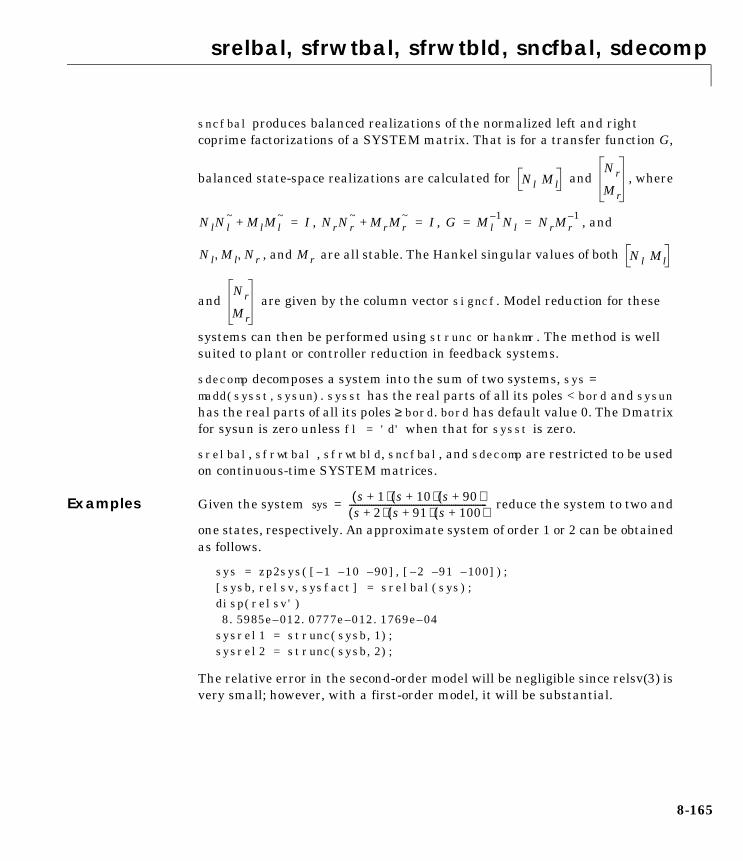
srelbal, sfrwtbal, sfrwtbld, sncfbal, sdecomp
sncfbal produces balanced realizations of the normalized left and rightcoprime factorizations of a SYSTEM matrix. That is for a transfer function G,
balanced state-space realizations are calculated for and , where
, , , and
, and are all stable. The Hankel singular values of both
and are given by the column vector signcf. Model reduction for these
systems can then be performed using strunc or hankmr. The method is wellsuited to plant or controller reduction in feedback systems.
sdecomp decomposes a system into the sum of two systems, sys =madd(sysst,sysun). sysst has the real parts of all its poles < bord and sysunhas the real parts of all its poles ≥ bord. bord has default value 0. The D matrixfor sysun is zero unless fl = 'd' when that for sysst is zero.
srelbal, sfrwtbal , sfrwtbld, sncfbal, and sdecomp are restricted to be usedon continuous-time SYSTEM matrices.
Examples Given the system reduce the system to two and
one states, respectively. An approximate system of order 1 or 2 can be obtainedas follows.
sys = zp2sys([–1 –10 –90],[–2 –91 –100]); [sysb,relsv,sysfact] = srelbal(sys); disp(relsv')8.5985e–012.0777e–012.1769e–04sysrel1 = strunc(sysb,1); sysrel2 = strunc(sysb,2);
The relative error in the second-order model will be negligible since relsv(3) isvery small; however, with a first-order model, it will be substantial.
Nl MlNr
Mr
NlNl~ MlMl
~+ I= NrNr
~ MrMr~
+ I= G Ml1– Nl NrMr
1–= =
Nl Ml Nr, , Mr Nl Ml
Nr
Mr
syss 1+( ) s 10+( ) s 90+( )
s 2+( ) s 91+( ) s 100+( )--------------------------------------------------------------=
8-165

srelbal, sfrwtbal, sfrwtbld, sncfbal, sdecomp
The reduced-order models of order k can be obtained in the frequency weightedcase as follows:
wt1 = nd2sys([1 10],[1 1]); [sys1,sig1] = sfrwtbal(sys,wt1); disp(sig1');4.1873e–014.6472e–031.0280e–04sys1hat = hankmr(sys1,sig1,1,'d'); syshat = sfrwtbld(sys1hat,wt1); disp(hinfnorm(mmult(msub(sys,syshat),minv(wt1))));4.6471e–034.6517e–03Inf
In this example the method nearly reaches the lower bound, but this cannot beclaimed in general.
Now consider approximating the unstable third order system,
using sncfbal. First the balanced realization of the normalized left coprimefactors is calculated, then this is truncated to two states and the reduced-ordersystem recovered from these normalized coprime factors using starp.
sys = zp2sys([],[0 1 –10],10); [sysnlcf,signcf] = sncfbal(sys); disp(signcf')9.6700e–015.2382e–012.3538e–02sysnlcfr = strunc(sysnlcf,2); sysr = starp(mmult([1;1],msub(sysnlcfr,[0 1])),–1,1,1)
If this is the transfer function of a plant to be controlled, then signcf(1) canbe used to predict the possible robust stability to perturbations in thecoprime factors, and the potential for model-order reduction of thecontroller is given by signcf(2:3), McFarlane and Glover (1989). In thisexample the maximum stablizable perturbations in the coprime factors isgiven by . Furthermore if a controller is designed
sys10
s s 1–( ) s 10+( )----------------------------------------=
1 signcf (1 )– 2 0.20770=
8-166

srelbal, sfrwtbal, sfrwtbld, sncfbal, sdecomp
to be optimal for the second-order reduced model, then its stability marginwill be at least
0.25477 – 2 * signcf(3) = 0.20770
Algorithm The algorithms are based on the results in the following papers.
Reference Anderson, B.D.O., and Y. Liu, “Controller reduction: Concepts andApproaches,” IEEE Transactions on Automatic Control, vol. AC–34, pp. 802–812, 1989.
Desai, U.B., and D. Pal, “A transformation approach to stochastic modelreduction,” IEEE Transactions on Automatic Control, vol. AC–29, pp. 1097–1100, 1984.
Glover, K., “Multiplicative approximation of linear multivariable systems witherror bounds,” Proceedings of the American Control Conference, Seattle, pp.1705–1709, 1986.
Latham, G.A., and B.D.O. Anderson, “Frequency-weighted optimal Hankelnorm approximation of state transfer functions,” Systems and Control Letters,vol. 5, pp. 229–236, 1985.
McFarlane, D.C., and K. Glover, Robust Controller Design using NormalisedCoprime Factor Plant Descriptions, Springer-Verlag, Lecture Notes in Controland Information Sciences, vol. 138, 1989.
Wang, W., and M.G. Safonov, “A tighter relative error bound for balancedstochastic truncation,” Systems and Control Letters, vol. 14, pp. 307–317, 1990.
See Also hankmr, sysbal, sresid, strunc
8-167

sresid, strunc
8sresid, struncPurpose Reduce the state dimension of a SYSTEM matrix
Syntax sysout = sresid(sys,ord)
sysout = strunc(sys,ord)
Description sresid residualizes the last states of a SYSTEM matrix sys. sresid accountsfor the DC contribution of the last columns and rows of the SYSTEM A matrixand the corresponding rows and columns of B and C. sresid assumes that theSYSTEM matrix is ordered so that the last states are to be residualized. If theorignal SYSTEM matrix is partitioned as
with A11 of size ord × ord, then the command
sysout = sresid(sys,ord)
results in
strunc truncates the states of the input system matrix sys, to a system withstate dimension equal to ord. strunc can be used in conjunction with the modelreduction routines sysbal and hankmr.
The resulting SYSTEM output matrix is
sysout = pss2sys ([A_11 B_1; C_1 D]);
p
A11 A12 B1
A21 A22 B2
C1 C2 D
=
sysout pss2sysA11 B1
C1 D
A12
C2
A221–
A21 B2 , ord–
=
8-168

sresid, strunc
Examples A two input, one output, four state SYSTEM is reduced down to a two input,one output, two state SYSTEM via sresid and strunc. The only differencebetween the two reduced-order systems is the value of their D matrices.
seesys(sys)–1.2e–01 0.0e+00 0.0e+00 0.0e+00 | 9.le–01 5.2e–01 0.0e+00 –3.2e–01 0.0e+00 0.0e+00 | 6.le–02 3.2e–01 0.0e+00 0.0e+00 –4.3e+00 0.0e+00 | 9.le–01 9.9e–01 0.0e+00 0.0e+00 0.0e+00 –9.9e+01 | 5.le–01 4.9e–01---------------------------------------|------------------- 2.7e–01 9.le–02 9.5e–01 7.4e–02 | 0.0e+00 0.0e+00
sys_strunc = strunc(sys,3);seesys(sys_strunc)–1.2e–01 0.0e+00 0.0e+00 | 9.le–01 5.2e–01 0.0e+00 –3.2e–01 0.0e+00 | 6.le–02 3.2e–01 0.0e+00 0.0e+00 –4.3e+00 | 9.le–01 9.9e–01-------------------------------|--------------------- 2.7e–01 9.le–02 9.5e–01 | 0.0e+00 0.0e+00
sys_resid = sresid(sys,3)seesys(sys_resid)
–1.2e–01 0.0e+00 0.0e+00 | 9.le–01 5.2e–01 0.0e+00 –3.2e–01 0.0e+00 | 6.le–02 3.2e–01 0.0e+00 0.0e+00 –4.3e+00 | 9.le–01 9.9e–01------------------------------|-------------------- 2.7e–01 9.le–02 9.5e–01 | 3.8e–04 3.7e–04
sysstrunc = strunc(sys,3); seesys(sysstrunc)sysresid = sresid(sys,3); seesys(sysresid)
See Also rifd, statecc, strans
8-169

starp
8starpPurpose Form the Redheffer star product of two VARYING/SYSTEM/CONSTANTmatrices. The star product is a generalization of a linear fractionaltransformation
Syntax sysout = starp(top,bot,dim1,dim2)
Description Connects the two matrices top and bot in the star product loop shown below.
The last dim1 outputs of top are fed to the first dim1 inputs of bot, and the firstdim2 outputs of bot are fed into the last dim2 inputs of top. The remaininginputs and outputs constitute sysout. By this description, the dimensions mustsatisfy
min(dim_out(top),dim_in(bot)) ≥ dim1
min(dim_out(bot),dim_in(top)) ≥ dim2
Further restrictions also arise
IF dim1 = dim_out(top) & dim2 = dim_out(bot)
THEN there are no outputs remaining in the interconnection
IF dim1 = dim_in(bot) & dim2 = dim_in(top)
THEN there are no inputs remaining in the interconnection
8-170
starp
In either case, it is unclear what to return as sysout, so it is returned empty.There is one exception to this situation. If either top or bot is a SYSTEMmatrix with a nonzero number of states, and all of the equalities in the both ofthe above IF conditions hold (hence there are no inputs or outputs in theinterconnection), then sysout will be a CONSTANT matrix, and will be the Amatrix governing the internal dynamics of the loop.
As usual, the only types of matrices that cannot be combined are SYSTEMmatrices with VARYING matrices.
If only two arguments are given (i.e., no dimensions specified),
out = starp(top,bot);
then the operation is equivalent to
dim1 = min(ynum(top),unum(bot)); dim2 = min(unum(top),ynum(bot)); out = starp(top,bot,dim1,dim2);
Algorithm The “µ-Tools Commands for LFTs” section in Chapter 4 provides details of thestar product formulae.
Reference Redheffer, R., “Inequalities for a matrix Riccati equation,” Journal ofMathematics and Mechanics, vol. 8, no. 3, 1959.
See Also sysic
8-171

statecc, strans
8statecc, stransPurpose Apply state-coordinate transformation to a SYSTEM matrix
Syntax sysout = statecc(sysin,t) [sysout,v] = strans(sys)
Description statecc applies a state coordinate transformation to the matrix, yielding a newSYSTEM matrix with
sysout = pck(tA*t,tB,C*t,D)
where A, B, C, and D are the state-space entries of the matrix sysin. t isrestricted to be square and have the same dimensions as the A matrix.
strans transforms the A matrix of sys in bidiagonal form with the complexconjugate roots in real 2 × 2 form. sysout contains the transformed SYSTEMmatrix and v is the transformation matrix. The A matrix is ordered byincreasing magnitude of its eigenvalues. strans calls the MATLAB eigcommand to do the reordering.
Note: strans may be inaccurate when a SYSTEM/CONSTANT matrix hasrepeated eigenvalues. This is due to the potential defective eigensystem, andthe lack of a full set of eigenvectors.
8-172
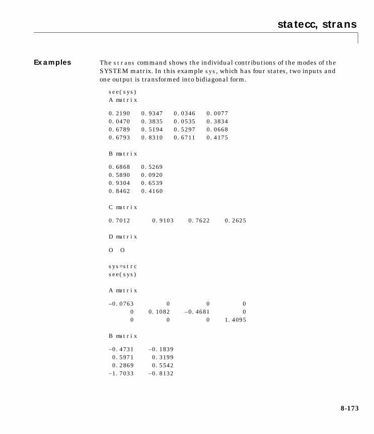
statecc, strans
Examples The strans command shows the individual contributions of the modes of theSYSTEM matrix. In this example sys, which has four states, two inputs andone output is transformed into bidiagonal form.
see(sys)A matrix
0.2190 0.9347 0.0346 0.00770.0470 0.3835 0.0535 0.38340.6789 0.5194 0.5297 0.06680.6793 0.8310 0.6711 0.4175
B matrix
0.6868 0.52690.5890 0.09200.9304 0.65390.8462 0.4160
C matrix
0.7012 0.9103 0.7622 0.2625
D matrix
O O
sys=strcsee(sys)
A matrix
–0.0763 0 0 0 0 0.1082 –0.4681 0 0 0 0 1.4095
B matrix
–0.4731 –0.1839 0.5971 0.3199 0.2869 0.5542–1.7033 –0.8132
8-173

statecc, strans
C matrix
–0.1150 0.0298 0.3214 –1.0477
D matrix
O O
See Also eig, sclin, sclout, veig
8-174
sysbal, hankmr
8sysbal, hankmrPurpose Calculate the balanced realization and optimal Hankel norm approximation ofa SYSTEM matrix. sysbal and hankmr are restricted to be used oncontinuous-time SYSTEM matrices whose poles have negative real part
Syntax [sysb,hanksv] = sysbal(sys,tol) [sysred,sysanti,siganti] = hankmr(sysb,hanksv,k,opt)
Description sysbal performs a truncated balanced realization of the input SYSTEMmatrix. The result is truncated to retain all Hankel singular values greaterthan tol. If tol is omitted then it is set to
max(hanksv(1) * 1.0–12,1.0–16)
The second output argument of sysbal is the vector hanksv, which contains theHankel singular values of the input system, sys. One method to get areduced-order model is to truncate the balanced system sysb using strunc.
hankmr returns sysred, the optimal Hankel norm approximation of order k tothe SYSTEM matrix, sysb, which is a balanced realization with Hankelsingular values hanksv and is of order n (n > k). The fourth optional inputargument, opt, may be omitted in which case sysanti contains the anti-causalterm such that the L∞ norm of (sysb – sysred – sysanti) is hanksv(k+1) orset to:
'a' when sysout also includes the anti-casual term, and sysanti=0'd' when sysout includes a D matrix to reduce the H∞ error norm of
(sys – sysout)
If the d option is set, the third output argument of hankmr is the vector siganti,which contains the Hankel singular values of the system, sysanti~. In thiscase
hanksv(k+1)≤||sys – sysred||∞≤hanksv(k+1)+sum(siganti)
8-175

sysbal, hankmr
Examples Given the system , reduce the system to two and
one states, respectively. First reduce the system to two states.
sys = zp2sys([–10 –90],[–2 –91 –100]); w = logspace(–1,3,100); sysg = frsp(sys,w); [syssb,sv]=sysbal(sys); svans =2.0613e–024.1136e–031.2663e–06sys2s = strunc(syssb,2);sys2sg = frsp(sys2s,w);sys2h = hankmr(syssb,sv,2);sys2hg = frsp(sys2h,w);vplot('bode',sys_g,sys2sg,sys2hg) tmp = 'Original 3 state system, 2 state Balanced ';tmp1 = 'and Hankel Model Reduction';title([tmp tmp1])
syss 10+( ) s 90+( )
s 2+( ) s 91+( ) s 10+( )-----------------------------------------------------------=
10-4
10-3
10-2
10-1
10-1 100 101 102 103
Log
Mag
nitu
de
Frequency (radians/sec)
-100
-80
-60
-40
-20
0
10-1 100 101 102 103
Pha
se (
radi
ans)
Frequency (radians/sec)
Original 3 state system, 2 state Balanced and Hankel Model Reduction
8-176
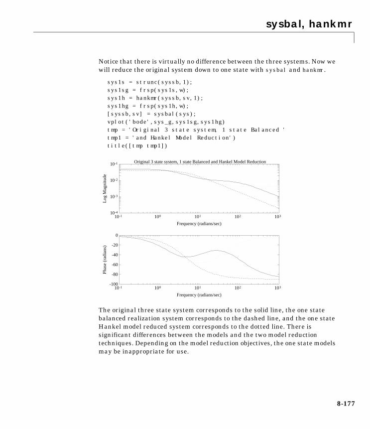
sysbal, hankmr
Notice that there is virtually no difference between the three systems. Now wewill reduce the original system down to one state with sysbal and hankmr.
sys1s = strunc(syssb,1);sys1sg = frsp(sys1s,w);sys1h = hankmr(syssb,sv,1);sys1hg = frsp(sys1h,w);[syssb,sv] = sysbal(sys);vplot('bode',sys_g,sys1sg,sys1hg) tmp = 'Original 3 state system, 1 state Balanced ' tmp1 = 'and Hankel Model Reduction') title([tmp tmp1])
The original three state system corresponds to the solid line, the one statebalanced realization system corresponds to the dashed line, and the one stateHankel model reduced system corresponds to the dotted line. There issignificant differences between the models and the two model reductiontechniques. Depending on the model reduction objectives, the one state modelsmay be inappropriate for use.
10-4
10-3
10-2
10-1
10-1 100 101 102 103
Log
Mag
nitu
de
Frequency (radians/sec)
-100
-80
-60
-40
-20
0
10-1 100 101 102 103
Pha
se (
radi
ans)
Frequency (radians/sec)
Original 3 state system, 1 state Balanced and Hankel Model Reduction
8-177

sysbal, hankmr
Reference K. Glover, “All optimal Hankel-norm approximations of linear multivariablesystems and their error bounds,” International Journal of Control, vol. 39, pp.1115–1193, 1984.
See Also sdecomp, sfrwtbal, sfrwtbld, sresid, srelbal, sresid
8-178

sysic
8sysicPurpose Form linear interconnections of CONSTANT and SYSTEM matrices (orCONSTANT and VARYING matrices)
Syntax sysic
Description µ-Tools provides a simple linear system interconnection program called sysic.It forms linear interconnections of CONSTANT and SYSTEM matrices (orCONSTANT and VARYING matrices, though this can require a lot of memory),by writing the loop equations of the interconnection.
Using sysic involves setting up several variables in the MATLAB workspace,and then running the M-file sysic. The variables that are defined delineate thedetails of the interconnection.
Variable DescriptionsA list and description of the variables required by sysic follow:
systemnames. This variable is a character string, which contains the names ofthe matrices used in the interconnection. The names must be separated byspaces and/or tabs, and there should be no additional punctuation. Each namedsystem must exist in the MATLAB workspace at the time the program sysicis run. The SYSTEM matrices names used within the sysic program arelimited to 10 characters. This limitation is due to the MATLAB 19 characterlimitation on the workspace variable names. That is, a SYSTEM matrix namedandygaryjohnkeithroy would be invalid.
inputvar. This variable is a character string, with names of the various externalinputs that are present in the final interconnection. The input names areseparated by semicolons, and the entire list of input names is enclosed insquare brackets [ ]. Inputs can be multivariable signals; for instance awindgust input, with three directions (x, y, and z) that can be specified by usingwindgust3. This means that there is a three variable input to theinterconnection called windgust. Alternatively, this could be specified as threeseparate, scalar inputs, say wingustx, windgusty, and windgustz. The orderthat the input names appear in the variable inputvar is the order that theinputs will be placed in the interconnection.
8-179
sysic
outputvar. This variable is a character string, describing the outputs of theinterconnection, which must be linear combinations of the subsystem outputsand the external inputs. Semicolons are used to separate the channels of theoutput variables. Between semicolons, signals can be added and subtracted,and multiplied by scalars. For multivariable subsystems, arguments withinparentheses specify which subsystem outputs are to be used and in what order.For instance plant (2:5,8,1,9:11) specifies outputs 2,3,4,5,8,1,9,10,11from the system plant. If no arguments are specified with a system, then it isassumed that all outputs are being used, and in the order they appear in thatsystem.
input_to_sys. Each subsystem named in the variable systemnames must have avariable set to define the inputs to the subsystem. If the system name iscontroller, then the variable that must be set should be calledinput_to_controller. It is specified in the same manner that the variableoutputvar is set, with inputs consisting of linear combinations of subsystemoutputs and external inputs. Separate channels are separated by semicolons,and the order of the inputs in the variable should match the order of the inputsin the system itself.
sysoutname. This character string variable is optional. If it exists in theMATLAB workspace when sysic is run, then the interconnection that iscreated by running sysic is placed in a MATLAB variable whose name is givenby the string in sysoutname. If this variable does not exist in the workspace,then the interconnection is automatically placed in the variable ic_ms.
cleanupsysic. After running sysic, all of the above variables, which describe theinterconnection, are left in the workspace. These will be automatically clearedif the optional variable cleanupsysic is set to the character string yes. Thedefault value of the variable is 'no' which does not result in any of the sysicdescriptions you defined to be cleared. The MATLAB matrices listed in thevariable systemnames are never automatically cleared.
Running sysic If the variables systemnames, inputvar, and outputvar are set, and for eachname name_i appearing in systemnames, the variable input_to_name_i is set,then the interconnection is created by running the M-file sysic. Depending onthe existence/nonexistence of the variable sysoutname, the resulting
8-180

sysic
interconnection is stored in your specified MATLAB variable, or the defaultMATLAB variable ic_ms.
Within sysic, a series of error-checking routines monitor the consistency andavailability of system matrices and their inputs. These routines provide a basiclevel of error detection to aid you in debugging. The input/output dimensions ofthe final interconnection are defined by inputvar and outputvar variables.
The syntax of sysic is limited, and for the most part is restricted to what isshown here. Some additional features are illustrated in the more complicateddemonstration problems. Note that you must keep track of input/outputvariables defined for the final interconnection structure.
Examples The HIMAT example provides another example of how to constructinterconnection systems from block diagram descriptions. The interconnectiondiagram below corresponds to the HIMAT design example.
Given that there are four SYSTEM matrices, named himat, wdel, wp, and k, inthe MATLAB workspace, each with two inputs, and two outputs. The following10 lines form the sysic commands to make the interconnection structureshown below, which is placed in the variable clp. You can execute these at thecommand line (as shown) or type them into an M-file. (Note that to run thisexample you must create the variables himat, wdel, wp and k.)
systemnames = ' himat wdel wp k ';inputvar = '[ pertin2;dis2]';outputvar = '[ wdel ;wp ]';input_to_himat = '[ k + pertin ]';input_to_wp = '[ dist + himat ]';input_to_wdel = '[ k ]';input_to_k = '[ –dist – himat ]';sysoutname = 'clp';cleanupsysic = 'yes';sysic;
8-181
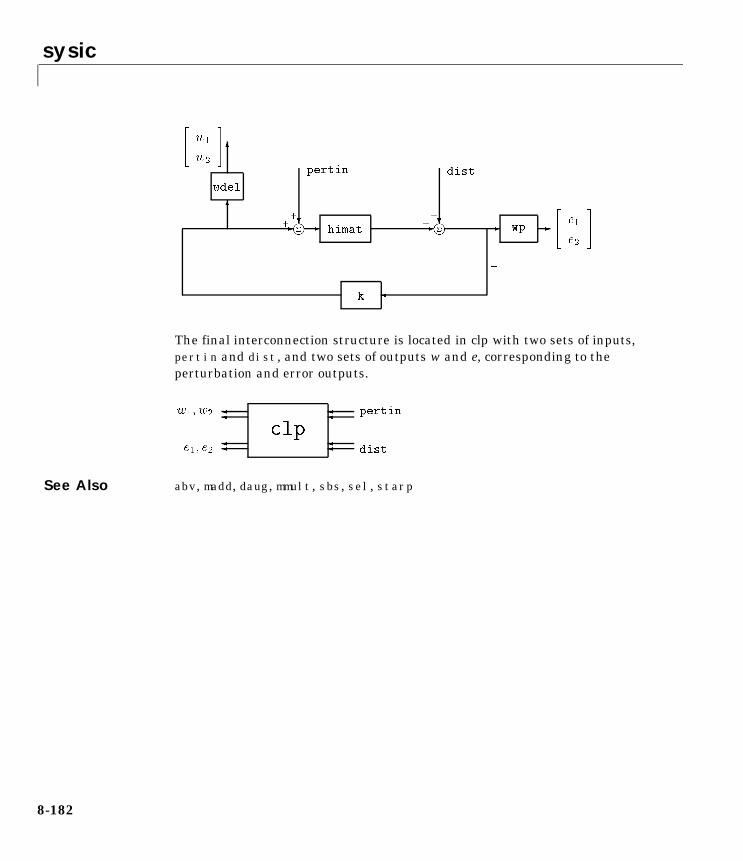
sysic
The final interconnection structure is located in clp with two sets of inputs,pertin and dist, and two sets of outputs w and e, corresponding to theperturbation and error outputs.
See Also abv, madd, daug, mmult, sbs, sel, starp
8-182

szeros
8szerosPurpose Transmission zeros of a SYSTEM matrix
Syntax veczeros = szeros(sys,epp)
Description szeros calculates the transmission zeros of the input SYSTEM matrix, sys.The output veczeros contains the vector of transmission zeros.
epp is an optional input argument which is used to test the closeness of thegeneralized eigenvalues of the randomly perturbed matrices. Its default valueis the machine epsilon. Occasionally zeros at infinity are displayed as verylarge values due to numerical accuracy problems.
For a square SYSTEM matrix, [A B; C D], the generalized eigenvalue testconsists of finding the roots of:
Algorithm For a square system, the transmission zeros are found via the generalizedeigenvalue problem described above. To solve for the transmission zeros of anonsquare SYSTEM matrix, additional random rows or columns areaugmented to the SYSTEM matrix to make it square and the correspondingzeros are found. This is done twice, and the unchanged generalizedeigenvalues, where the difference between the eigenvalues is less than epp, areconsidered to be the transmission zeros of the SYSTEM matrix.
Reference Laub, A.J., and B.C. Moore, “Calculation of transmission zeros using QZtechniques,” Automatica, vol. 14, pp. 557–563, 1978.
See Also spoles
det A λI– B
C D
0=
8-183
trsp, dtrsp, sdtrsp
8trsp, dtrsp, sdtrspPurpose Compute the time response of linear system
Syntax y = trsp(sys,u,tfinal,int,x0) y = dtrsp(dsys,u,T,tfinal,x0) [output,y,u] = sdtrsp(sys,k,input,T,tfinal,int,x0,z0)
Description trsp computes the time response of the continuous-time system, sys, with theinput, u. The input, u, is a VARYING matrix, which contains the input signalvector at certain points in time. The input can be irregularly spaced in theindependent variable or a constant, in which case it is assumed to occur at t =0.
The final time, tfinal, is an optional argument. If omitted, it defaults to themaximum time in u. The time response is calculated as though the input is aconstant value between the points specified in u. If tfinal is greater than thelargest independent variable in u, the input is held at the last value in u.
For continuous-time evaluation (trsp), you can optionally specify anintegration time with the variable int. If this is omitted, or is equal to zero, anappropriate value is calculated and displayed. The calculated integration timedepends on the minimum spacing in the input and the fastest dynamics in sys.int will also be the independent variable step size in the regularly spacedoutput, y. If a coarser output is adequate, it can be obtained with the functionvdcmate.
Initial conditions can optionally be specified with the argument, x0. Thisspecifies the state vector at the first time point in the input vector. If x0 isomitted, or is a zero scalar, then it is assumed to be a zero vector.
trsp interpolates the input with a zero-order hold of step size equal to int,discretizes the output at this same step size, and calculates the response fromthe initial time to tfinal in steps of int.
dtrsp calculates the response for a discrete-time system, dsys. The time (forthe independent variable) between discrete indices is T. If the input is notregularly spaced at intervals of time T, it is interpolated. tfinal and x0 behavein the same manner as for trsp.
sdtrsp calculates a sampled-data time response for a closed-loop system witha continuous generalized plant (sys) and a discrete controller (K). Theinterconnection is illustrated below.
8-184

trsp, dtrsp, sdtrsp
The signals, output, y, and u are calculated. T is the sampled-data controllersample time, and you have the same input and tfinal options as the trspfunction. Similarly, an integration step size, int, can optionally be specified forthe continous part of the simulation. Initial conditions can be specified for sys(x0) and K (z0).
Examples A simple SISO system illustrates the use of trsp. This example shows theconsequences of the input being assumed to be constant between time points.
sys = pck(–1,1,1); minfo(sys)system:1 states1 outputs1 inputsu = vpck([0:10:50]',[0:10:50]'); y = trsp(sys,u,60);integration step size: 0.1interpolating input vector (zero order hold)minfo(y)varying:601 pts1 rows1 colsvplot(u,'–.',y,'–') xlabel('time: seconds') text(10,20,'input') text(25,10,'output')
8-185

trsp, dtrsp, sdtrsp
At first glance the output does not seem to be consistent with the plotted input.Remember that trsp assumes that the input is held constant between specifiedvalues. The vplot and plot commands display a linear interpolation betweenpoints. This can be more clearly seen by displaying the input signalinterpolated to at least as small a step size as the default integration step (here0.1 seconds).
vplot(u,'–.',vinterp(u,0.1),'--',y,'–') xlabel('time: seconds') text(5,44,'dash-dot: input') text(5,40,'dashed: interpolated input') text(5,36,'solid: output')
0
5
10
15
20
25
30
35
40
45
50
0 10 20 30 40 50 60
Time: seconds
input
output
8-186

trsp, dtrsp, sdtrsp
The staircase nature of the input is now evident. If you really want to have aramp input, the function vinterp also provides linear interpolation. A linearlyinterpolated input is used in the following example.
uramp = vinterp(u,0.1,60,1); minfo(uramp)varying:601 pts1 rows1 colsyramp = trsp(sys,uramp);integration step size: 0.1vplot(uramp,'–.',yramp,'–') xlabel('time: seconds') text(20,15,'output') text(12,20,'input')
0
5
10
15
20
25
30
35
40
45
50
0 10 20 30 40 50 60
Time: seconds
dash-dot: input
solid: output
dashed: interpolated input
8-187

trsp, dtrsp, sdtrsp
Note that because the input is regularly spaced, with spacing less than or equalto the default integration time, the input is not interpolated by trsp. Since nofinal time was specified in the trsp argument list, and 60 seconds was specifiedto vinterp as the final time, this becomes the last time in the input vectoruramp.
To illustrate the use of dtrsp, a bilinear transformation generates a digitalsystem. The sample time is chosen as 1 second. The output is plotted against a1 second interpolation of the input.
T = 1; dsys = tustin(sys,T); ydig = dtrsp(dsys,u,T); vplot(ydig,'–',vinterp(u,1),'–.') xlabel('time: seconds')
0
5
10
15
20
25
30
35
40
45
50
0 10 20 30 40 50 60
output
input
Time: seconds
8-188

trsp, dtrsp, sdtrsp
To illustrate the use of sdtrsp, consider the application of a discrete controllerto a double integrator. A continuous plant and a discrete controller are created.A sample and hold equivalent of the plant is formed and the discreteclosed-loop system is calculated. Simulating this with dtrsp gives the systemresponse at the sample points. sdtrsp is then used to calculate the intersamplebehavior.
P = nd2sys(1,[1,0,0]); T = 1.0/20; C=pck([–1.5 T/4; –2/T -.5],[ .5 2;1/T 1/T], ... [–1/T2 –1.5/T], [1/T2 0]);
The closed-loop digital system is now set up.
Pd = samhld(P,T); systemnames = 'Pd C'; inputvar = '[ref]'; outputvar = '[Pd]'; input_to_Pd = '[C]'; input_to_C = '[ref ; Pd]'; sysoutname = 'dclp'; cleanupsysic = 'yes'; sysic;
0
5
10
15
20
25
30
35
40
45
50
0 10 20 30 40 50 60
Time: seconds
8-189
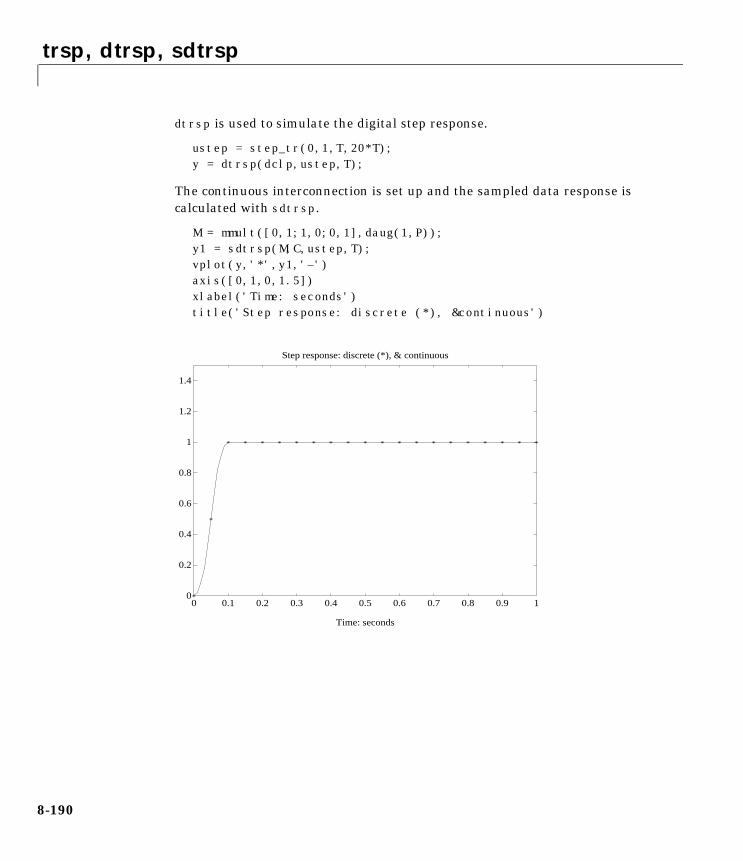
trsp, dtrsp, sdtrsp
dtrsp is used to simulate the digital step response.
ustep = step_tr(0,1,T,20*T); y = dtrsp(dclp,ustep,T);
The continuous interconnection is set up and the sampled data response iscalculated with sdtrsp.
M = mmult([0,1;1,0;0,1],daug(1,P)); y1 = sdtrsp(M,C,ustep,T); vplot(y,'*',y1,'–') axis([0,1,0,1.5]) xlabel('Time: seconds') title('Step response: discrete (*), &continuous')
0
0.2
0.4
0.6
0.8
1
1.2
1.4
0 0.1 0.2 0.3 0.4 0.5 0.6 0.7 0.8 0.9 1*
*
* * * * * * * * * * * * * * * * * * *
Time: seconds
Step response: discrete (*), & continuous
8-190

trsp, dtrsp, sdtrsp
Now we look at the effect of a nonzero initial condition in the continuoussystem. Note how examining the system at only the sample points willunderestimate the amplitude of the overshoot.
y2 = sdtrsp(M,C,vpck(1,0),T,1,0,[1;0]); vplot(y1,'--',y2,'–') axis([0,1,0,1.5]) xlabel('Time: seconds') title('Step response: non zero initial condition')
Finally, we will examine the effect of a sinusoidal disturbance at thecontinuous plant output. This controller has not been designed to reject such adisturbance and the system does not contain anti-aliasing filters. Simulatingthe effect of anti-aliasing filters is easily accomplished by including them in thecontinuous interconnection structure.
M2 = mmult([0,1,1;1,0,0;0,1,1],daug(1,1,P)); dist = sin_tr(41,0.1,0.001,1); [dat,datptr,t] = vunpck(dist); input = abv(vpck(ones(t),t),dist); [y3,meas,act] = sdtrsp(M2,C,input,T); vplot(y3,'–',input,'--')
0
0.2
0.4
0.6
0.8
1
1.2
1.4
0 0.1 0.2 0.3 0.4 0.5 0.6 0.7 0.8 0.9 1
Time: seconds
Step response: non zero initial condition
8-191

trsp, dtrsp, sdtrsp
xlabel('Time: seconds') title('Step response: disturbance (dashed) & output (solid)')
Algorithm trsp first calculates an integration time (or uses the specified integration time)to determine the sample time at which to discretize the continuous-timesystem. The integration time is taken to be the inverse of 10 times the fastestmode of the input system. The input vector is interpolated at each sample timevia a zero-order hold, and then a sample-hold of the input continous system isperformed. Finally the time response of the system is performed via a for loopat each integration time step. dtrsp is provided a discrete time system and asample time. dtrsp first interpolates the input vector via a zero-order hold andthen determines the time response via a for loop at each sample time.
Caution: Systems with fast dynamics lead to very small integration times.This is both time consuming and requires a significant amount of storage. Werecommend you residualize the fastest modes of the system, which does notaffect the time response. This can be done with the µ-Tools command sresid.
See Also cos_tr, siggen, sin_tr, step_tr, sysbal, vdcmate, vinterp
-0.2
0
0.2
0.4
0.6
0.8
1
1.2
1.4
0 0.1 0.2 0.3 0.4 0.5 0.6 0.7 0.8 0.9 1
Time: seconds
Step response: disturbance (dashed) & output (solid)
8-192

tustin
8tustinPurpose Create a discrete-time version of a continuous-time SYSTEM matrix using abilinear or prewarped tustin transformation
Syntax dsys = tustin(csys,T,prewarpf)
Description The packed continuous SYSTEM matrix, csys, is converted into a discrete-timeSYSTEM matrix, dsys, using a bilinear transformation with prewarping. Theargument T is the sample time, in seconds. prewarpf is the prewarp frequencyin rads/sec. prewarpf is an optional argument, and if omitted, or equal to zero,a bilinear transformation is performed instead.
The resulting discrete system, dsys, has the same transfer function at thecontinuous system, csys, at the prewarp frequency. Choosing a prewarpfrequency close to the crossover frequency is often appropriate for a controlsystem. Choosing a prewarp frequency too close to the Nyquist frequency (1/2T)can result in severe distortion at the lower frequencies. In the extreme, ifprewarp is greater than or equal to π/T, the discrete system can be unstable.
Note that the transfer function is preserved at zero frequency with a bilineartransformation, hence having the input variable prewarpf equal to zero toindicate a bilinear transformation is therefore consistent.
Examples Create a second-order system with a resonance at 1 rad/sec.
a = [–.1,1;–1,-0.05]; b = [1;1]; c = [–0.5,0] sys = pck(a,b,c); minfo(sys)system:2states1 outpus1 inputsomega = logspace(–2,2,100); omega2 =[ [0.05:0.1:1.5] [1.6:.5:20] [0.9:0.01:1.1] ]; omega = sort([omega omega2]); sys_g = frsp(sys,omega);
8-193

tustin
Choose a sample frequency of 20 rads/sec and discretize the system with abilinear transformation.
T = 2*pi/20; dsys = tustin(sys,T); dsys_g = frsp(dsys,omega,T); vplot('bode',sys_g,dsys_g,'–.'); title('Continuous system (solid), bilinear equivalent (dot-dash)')
The bilinear approximation is accurate up to about 2 rads/sec. This exampleshows the effect of choosing a higher prewarping frequency, specifically 5 rads/sec.
prewarpf = 5; dsys2 = tustin(sys,T,prewarpf); dsys2g = frsp(dsys2,omega,T); vplot('bode',sys_g,dsys2_g,'–.'); title('Continuous system (solid), tustin equivalent (dot-dash)')
10-3
10-2
10-1
100
101
10-2 10-1 100 101 102
Log
Mag
nitu
de
Frequency (radians/sec)
-4
-2
0
2
4
10-2 10-1 100 101 102
Pha
se (
radi
ans)
Frequency (radians/sec)
Continuous system (solid), bilinear equivalent (dot-dash)
8-194

tustin
Note the distortion in the frequency of the lightly damped peak. At 5 rads/secboth the continuous and discrete systems have the same transfer function.
sys_5 = vunpck(frsp(sys,5)); dsys2_5 = vunpck(frsp(dsys2,5,T)); err = abs(dsys2_5 – sys_5); fprintf('error at %g rad/sec is : %g ',prewarpf,err);error at 5 rad/sec is : 1.155158e–17
This example highlights the distortion possible. If the frequency of theresonance had been critical to the design, a prewarp frequency of 1 rad/secwould have been more appropriate.
As an alternative, you can generate a filter/controller design using a warpedfrequency scale in the continuous domain. Then the transformation to thediscrete domain would result in the correct transfer function at the frequenciesof interest.
Algorithm The prewarped tustin transformation is based on the equation:
10-3
10-2
10-1
100
101
10-2 10-1 100 101 102
Log
Mag
nitu
de
Frequency (radians/sec)
-4
-2
0
2
4
10-2 10-1 100 101 102
Pha
se (
radi
ans)
Frequency (radians/sec)
Continuous system (solid), Tustin equivalent (dot-dash)
8-195

tustin
where
Reference Oppenheim, A.V., and R.W. Schafer, Digital Signal Processing, Prentice Hall,New Jersey, 1975.
See Also dtrsp, frsp, samhld, tustin
csys A BC D
, using the prewarped Tustin transform=
dsysAdisc Bdisc
Cdisc Ddisc
,=
α prewrapfT*prewarpf/2( )tan
-----------------------------------------=
Adisc I 1α---A+( ) * I 1
α--- A–( )
1–=
Bdisc2α---( )
12---
* I 1α---A–( )
1–* B=
Cdisc2α---( )
12---
* C * I 1α---A–( )
1–=
Ddisc D 1α---+ * C * I 1
α---A–
1–( ) * B=
8-196
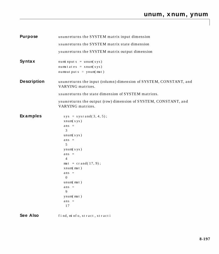
unum, xnum, ynum
8unum, xnum, ynumPurpose unum returns the SYSTEM matrix input dimension
xnum returns the SYSTEM matrix state dimension
ynum returns the SYSTEM matrix output dimension
Syntax numinputs = unum(sys) numstates = xnum(sys) numoutputs = ynum(mat)
Description unum returns the input (column) dimension of SYSTEM, CONSTANT, andVARYING matrices.
xnum returns the state dimension of SYSTEM matrices.
ynum returns the output (row) dimension of SYSTEM, CONSTANT, andVARYING matrices.
Examples sys = sysrand(3,4,5); xnum(sys) ans = 3 unum(sys) ans = 5 ynum(sys) ans = 4 mat = crand(17,9); xnum(mat) ans = 0 unum(mat) ans = 9 ynum(mat) ans = 17
See Also find, minfo, xtract, xtracti
8-197

vabs, vimag, vreal, vfloor, vceil
8vabs, vimag, vreal, vfloor, vceilPurpose Perform element-by-element operations on CONSTANT and VARYINGmatrices
Syntax matout = vabs(matin) matout = vimag(matin) matout = vreal(matin) matout = vfloor(matin) matout = vceil(matin)
Description This set of commands allows standard element-by-element operations onCONSTANT/VARYING matrices. These commands are identical to abs, imag,real, floor, and ceil but also work on VARYING matrices.
A general element-by-element command, vebe, allows all standard arithmeticMATLAB element commands that have only one input argument.
Examples Construct a complex VARYING matrix and find the magnitude of the entriesand the real parts.
see(matin)1 row 2 columnsiv = .20.2190 – 0.4379i0.6789 – 1.3577iiv = .70.0470 – 0.0941i0.6793 – 1.3586i
vabs element-by-element absolute value of a VARYING matrix
vimag element-by-element imaginary part of a VARYING matrix
vreal element-by-element real part of a VARYING matrix
vfloor element-by-element floor of a VARYING matrix
vceil element-by-element ceiling of a VARYING matrix
8-198

vabs, vimag, vreal, vfloor, vceil
see(vabs(matin))1 row 2 columnsiv = .20iv = .70.10521.5190see(vreal(matin))1 row2 columnsiv = .20.21900.6789iv = .70.04700.6793
Use pkvnorm to find the maximum element magnitude of the VARYINGmatrix.
pkvnorm(matin,inf)1 row2 columnsans =1.5190
This agrees with the maximum magnitude of matin(1,1) associated with thesecond independent variable.
See Also vdet, vdiag, vebe, veval
8-199

vdet, vdiag, vexpm, vrcond
8vdet, vdiag, vexpm, vrcondPurpose Calculate determinant, diagonal, matrix exponential and estimate of conditionnumber of a CONSTANT or VARYING matrix
Syntax out = vdet(matin) out = vdiag(matin) out = vexpm(matin) out = vrcond(matin)
Description These commands operate on square, CONSTANT and VARYING matrices andthey are identical to the MATLAB commands det, diag, exp, and rcond onCONSTANT matrices.
vdet of a square, VARYING matrix, returns matout, which is a VARYING1 × 1 matrix, containing the value of the determinant of matin at eachindependent variable value.
vdiag of a square, VARYING matrix, returns matout, which is a VARYINGmatrix of size min(size(matin)) × 1, containing the diagonal elements ofmatin at each independent variable.
vexpm of a square, VARYING matrix, returns matout, which is a VARYINGmatrix of the same size as matin, containing the matrix exponential of matin.The MATLAB command expm, which is called, uses a Pade expansion afterscaling matin to calculate the exponential.
vrcond of a square, VARYING matrix, returns matout, which is an estimate ofthe condition number of a matrix.
Examples vdet and vrcond work similarly to their MATLAB counterparts, det andrcond, but on square VARYING matrices as shown below.
see(matin)2 rows 2 columnsiv = 2.30.04750.32820.73610.6326iv = 5.60.75640.36530.99100.2470matout = vdet(matin);
8-200

vdet, vdiag, vexpm, vrcond
see(matout)1 row 1 columniv = 2.3–0.2116iv = 5.6–0.1752see(vrcond(matin))1 row 1 columniv = 2.30.1907iv = 5.60.0848
See Also det, diag, expm, rcond
8-201

vebe
8vebePurpose Perform element-by-element operations on CONSTANT and VARYINGmatrices
Syntax out = vebe('oper',matin)
Description The vebe function allows any single argument MATLAB element-by-elementarithmetic command to operate on a VARYING matrix. The first inputargument, oper, is the character string defining the MATLABelement-by-element command and matin is the VARYING matrix on which thecommand is applied. vebe calls the MATLAB eval command to execute thestring command. Some standard MATLAB comands compatible with vebe aresin, abs, real, imag, and gamma.
Examples In this example of vebe, the real part of a matrix is found along with gamma ofeach matrix element.
see(matin)3 rows 3 columnsiv = 4.2
1.0000 + 2.0000i 1.0000 + 2.0000i 1.0000 + 2.0000i2.0000 + 4.0000i 2.0000 + 4.0000i 2.0000 + 4.0000i3.0000 + 6.0000i 3.0000 + 6.0000i 3.0000 + 6.0000i
iv = 11.01
4.0000 + 8.0000i 4.0000 + 8.0000i 4.0000 + 8.0000i5.0000 + 10.0000i 5.0000 + 10.0000i 5.0000 + 10.0000i6.0000 + 12.0000i 6.0000 + 12.0000i 6.0000 + 12.0000i
matout = vebe('real',matin);see(matout)3 rows 3 columns
8-202

vebe
iv = 4.21 1 12 2 23 3 3
iv = 11.014 4 45 5 56 6 6see (vebe ('gamma ', matin))3 rows 3 columns
iv = 4.21 1 11 1 12 2 2
iv = 11.01 6 6 6 24 24 24120 120 120
See Also eval, vabs, vceil, veval, vfloor, vimag, vreal
8-203

veig
8veigPurpose Calculate eigenvalues and eigenvectors of CONSTANT and VARYINGmatrices
Syntax evals = veig(matin) [evecs,evals] = veig(matin) [evecs,evals] = veig(matin,'nonbalance') [evecs,evals] = veig(mat1,mat2)
Description veig is identical to MATLAB’s command eig, but works on VARYINGmatrices. veig solves for the eigenvalues (evals) and optionally theeigenvectors (evecs) of the input matrix matin. veig works only on squareCONSTANT or VARYING matrices. Depending on the input arguments, thefollowing operations are performed:
evals = veig(matin) returns a VARYING vector evals containing theeigenvalues of the VARYING matrix matin for each independent variable.
[evecs,evals] = veig(matin) returns the VARYING diagonal matrix evalsand a square VARYING matrix evecs whose columns are the correspondingeigenvectors for each independent variable.
[evecs,evals] = veig(matin,'nobalance') is the same as the abovecommand without performing a preliminary balancing step. Balancing amatrix, which has very small entries due to round off error, can lead toincorrect eigenvectors.
[evecs,evals] = veig(mat1,mat2) returns a VARYING diagonal matrix ofgeneralized eigenvalues evals and the corresponding values of generalizedright eigenvectors evecs associated with each independent variable. mat1 andmat2 can be CONSTANT or VARYING matrices. If either is CONSTANT, thenthat same matrix is used in the generalized eigenvalue solution for eachindependent variable. If they are both VARYING matrices, then they musthave the same independent variables.
8-204

veig
Examples Create a 2 × 2 random VARYING matrix and find its eigenvalues.
see(matin)2 rows 2 columns
iv = 0.10.9304 0.52690.8462 0.0920iv = 0.40.6539 0.70120.4160 0.9103evals = veig(matin);see(evals)2 rows1 column
iv = 0.1 1.2996 –0.2772
iv = 0.4 0.2270 1.3372
Using the same matrix and creating another two by two VARYING matrix,solve the generalized eigenvalue problem with these two matrices.
mat1 = matin; mat2 = vpck([4*eye(2);3*eye(2)],[.1 .4]); [evecs,evals] = veig(mat1,mat2);see(evecs)2 rows 2 columns
iv = 0.1 0.8190 –0.3999 0.5738 0.9166
iv = 0.4 0.8542 0.7162–0.5200 0.6979see(evals)
8-205

veig
2 rows 2 columns
iv = 0.1 0.3249 0 0 –0.0693iv = 0.4 0.0757 0 0 0.4457
Algorithm veig calls the MATLAB eig command.
See Also eig, indvcmp, svd, vsvd, vpoly, vroots
8-206
veval
8vevalPurpose Evaluate general functions of CONSTANT, SYSTEM, and VARYING matrices
Syntax [out1,out2,out3,...]= veval('oper',in1,in2,in3,...)
Description The veval function evaluates the command oper on the input matrices. vevalworks like feval but on collections of VARYING, CONSTANT, and SYSTEMmatrices. 'oper' is a character string with the name of a MATLAB function(user written, or MATLAB supplied). The function is applied to each inputargument at the independent variable’s values. Any CONSTANT or SYSTEMmatrix is held at its value while the sweep through the independent variable isperformed. veval is currently limited to 10 output arguments, and 13 inputarguments. These are both easily changeable. veval can be used to generateand manipulate VARYING, SYSTEM matrices or VARYING matrices whoseelements are themselves VARYING matrices. Arbitrary nesting of VARYINGmatrices is possible.
The veval function is very useful for rapid prototyping of customizedcommands employing VARYING matrices.
Examples To show the flexibility of veval, two random SYSTEM matrices areconstructed. The poles of each SYSTEM are determined with the spolescommand.
sys1 = sysrand(2,1,1); sys2 = sysrand(2,1,1);spoles(sysl)ans = 0.1577 0.7405spoles(sys2)ans = 0.6273–0.5661
These two SYSTEM matrices are combined to form a VARYING matrix, vsys.The veval command is used to find poles of the VARYING matrix, which
8-207

veval
consists of the two SYSTEM matrices. A SYSTEM matrix is associated witheach independent variable.
vsys = vpck([sysl;sys2],[1 2]);vsyspoles = veval('spoles',vsys);see(vsyspoles)2 rows1 column
iv = 1 0.1577 0.7405
iv = 2 0.6273–0.5661
See Also eval, feval, vebe
8-208

vfft, vifft, vspect
8vfft, vifft, vspectPurpose Calculate FFTs, inverse FFTs, and perform spectral analysis on VARYINGmatrices
Syntax yfreq = vfft(ytime,n) ytime = vifft(yfreq) P = vspect(x,m,noverlap,'window') P = vspect(x,y,m,noverlap,'window')
Description vfft implements the MATLAB fft command on VARYING matrix structures.A one-dimensional FFT of length n is performed on each element of theVARYING matrix ytime. It is assumed that the independent variable is inunits of seconds. The independent variables are regularly spaced — only thefirst interval is used to determine the frequency scale. yfreq is returned withthe independent variable, frequency, in radians/second.
vifft performs the inverse FFT. This is done with the MATLAB commandifft(yfreq) for each element of the VARYING matrix.
vspect is the VARYING matrix structure equivalent of the Signal ProcessingToolbox command, spectrum. For algorithmic details, see the spectrumcommand. Note that vspect gives you the option of specifying a window for thedata. For example, using the string hamming as the fifth argument generates awindow with the command window = hamming(n);. hamming is an M-file in theSignal Processing Toolbox. You can use custom windows by specifying thename as the window argument.
In the case of the spectrum of a single signal, the command
P = vspect(x,m,noverlap,'window');
will return a VARYING matrix, P, containing the power spectral density of x.Note that x, and therefore P, can be a matrix of signals. In the case of thespectrum, and cross-spectrum, of two signals, the command
P = vspect(x,y,m,noverlap,'window');
will return a VARYING matrix, P, with the following five columns.
[Pxx Pyy Pxy Txy Cxy]
8-209

vfft, vifft, vspect
These are given below.
The signal x, must be scalar (i.e., a one row, one column, VARYING matrix). ycan be a vector signal. The row dimension of p is the same as that of y. vspectcan do single-input, multiple-output (SIMO) identification. This is illustratedin the following example. Refer also to the example in the Tutorial chapter.
vfft, vifft, and vspect have not been optimized for speed. The appropriaterow and column data is extracted from the VARYING matrices with the µ-Toolscommands, sel and xtract. sbs and abv are used to create the final output.
Examples A single-input two-output system is generated as an identification example.This example is only a simple illustration of some of the frequency domaintechniques available.
a1 = [–.1,1;–1,-0.05]; b1 = [1;1]; c1 = [–0.5,0]; sys1 = pck(a1,b1,c1); a2 = [–.1,0.5;-0.5,-0.1]; b2 = [1;1]; c2 = [–0.5,0]; sys2 = pck(a2,b2,c2); sys = abv(sys1,sys2); minfo(sys)system:4 states2 outputs1 inputs
Now a random input signal is created.
t = [0:0.05:102.35]; u = siggen('0.5-rand(size(t))',t); minfo(u)varying:2048 pts1 rows1 cols
Pxx Power spectral density of x
Pyy Power spectral density of y
Pxy Cross spectral density
Txy Complex transfer function between x and y
Cxy Coherence function between x and y
8-210
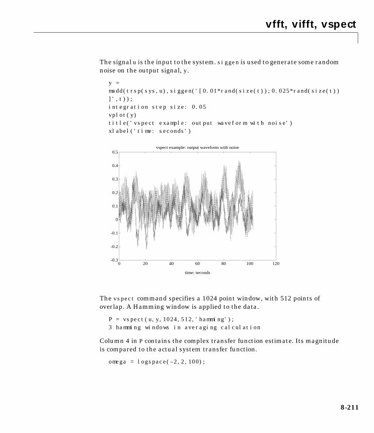
vfft, vifft, vspect
The signal u is the input to the system. siggen is used to generate some randomnoise on the output signal, y.
y = madd(trsp(sys,u),siggen('[0.01*rand(size(t));0.025*rand(size(t))]',t));integration step size: 0.05vplot(y) title('vspect example: output waveform with noise') xlabel('time: seconds')
The vspect command specifies a 1024 point window, with 512 points ofoverlap. A Hamming window is applied to the data.
P = vspect(u,y,1024,512,'hamming');3 hamming windows in averaging calculation
Column 4 in P contains the complex transfer function estimate. Its magnitudeis compared to the actual system transfer function.
omega = logspace(–2,2,100);
-0.3
-0.2
-0.1
0
0.1
0.2
0.3
0.4
0.5
0 20 40 60 80 100 120
vspect example: output waveform with noise
time: seconds
8-211

vfft, vifft, vspect
omega2 =[ [0.05:0.1:1.5] [1.6:.5:20] [0.9:0.01:1.1] ]; omega = sort([omega omega2]); sys_g = frsp(sys,omega); vplot('liv,lm',sel(P,1:2,4),sys_g);Warning: Data includes a number that is negative or zero.The LOG of this results in NaN or Infinity and is not shown on plot.title('vspect example: transfer function estimation ') ylabel('magnitude') xlabel('frequency: rad/sec')
Algorithm vfft, vifft, and vspectrum call the MATLAB commands fft and ifft.
Reference Ljung, L., System Identification: Theory for the User, Prentice Hall, NewJersey, 1987.
Oppenheim, A.V., and R.W. Schafer, Digital Signal Processing, Prentice Hall,New Jersey, 1975.
See Also fft, ifft, spectrum
10-3
10-2
10-1
100
101
10-2 10-1 100 101 102
vspect example: transfer function estimation
mag
nitu
de
frequency: rad/sec
8-212

vfind
8vfindPurpose Unary find function across independent variable
Syntax [iv_value,iv_index] = vfind(condition,mat)
Description vfind is a unary find function that searches across independent variablevalues. The condition to be tested can be any valid MATLAB conditionalstatement, using the string mat to identify the matrix, and iv as theindependent variable’s value. Both the values and indices of the applicableindependent variables are returned.
Examples Suppose that matin is a VARYING matrix. In order to find those entries forwhich the product of the norm of the matrix, and the independent variable isgreater than 2, use vfind as follows:
[iv_value,iv_index] = vfind('iv*norm(mat)>2',matin); matpropv = xtract(matin,iv_value); % extract by value matpropi = xtracti(matin,iv_index); % extract by index pkvnorm(msub(matpropv,matpropi)) % compare – both are the same
See Also find, xtract, xtracti
8-213

vinterp, vdcmate
8vinterp, vdcmatePurpose Interpolate or decimate VARYING matrices
Syntax vout = vinterp(vin,stepsize,finaliv,order) vout = vinterp(vin,varymat,order) vout = vdcmate(vin,spacing)
Description In the first form, vinterp produces a regularly spaced interpolated version ofthe input VARYING matrix. The input arguments are
The end value for the independent variable may or may not be in the actualoutput. This is consistent with the usual MATLAB treatment of regularlyspaced vectors. For example, consider
iv = [1:2:6];disp(iv)1 3 5
Note that the value of 6 does not appear in the vector.
In the second form, vinterp produces a VARYING matrix vout that is aninterpolated version of vin. The independent variables of vout are the same asthe independent variables of varymat. The input arguments are:
varymat
VARYING matrix with desired independent variables
order
type of interpolation (optional, default = 0)
0 zero-order hold
1 linear interpolation
stepsize independent variable stepsize
finaliv end value for independent variable (Optional: the default isthe final independent variable in the input)
order type of interpolation (optional, default = 0)0 zero-order hold1 linear interpolation
8-214

vinterp, vdcmate
vdcmate decimates the VARYING matrix vin, whose independent variablemust be linearly spaced and in ascending order. If spacing has a value of n,then the output contains only the matrices corresponding to every nthindependent variable of the input. If no spacing is specified, the default is 10.
Examples siggen creates a sinewave. This is effectively sampled by vdcmate and theninterpolated by vinterp. Note that the default interpolation is a zero-orderhold, giving a stair-step output, yi. If a linearly interpolated output werespecified, it would look identical to yd since the MATLAB plot commanddisplays a linear interpolation.
timebase = [0:0.005:20]; y = siggen('sin(2*pi*t)',timebase); minfo(y)varying:4001 pts1 rows1 colsyd = vdcmate(y,210); minfo(yd)varying:20 pts1 rows1 colsyi = vinterp(yd,0.005,20,0); minfo(yi)varying:4001 pts1 rows1 colsaxis([0,20,–1.5,1.5]) vplot(y,yd,yi) title('vdcmate/vinterp example: undersampled sine wave') xlabel('time: seconds')
8-215

vinterp, vdcmate
See Also dtrsp, sort, sortiv, tackon, trsp
-1.5
-1
-0.5
0
0.5
1
1.5
0 2 4 6 8 10 12 14 16 18 20
vdcmate/vinterp example: undersampled sine wave
time: seconds
8-216

vldiv, vpinv, vrdiv
8vldiv, vpinv, vrdivPurpose Determine left division, pseudo-inverse and right division of a CONSTANT orVARYING matrix
Syntax out = vldiv(mat1,mat2) out = vpinv(mat,tol) out = vrdiv(mat1,mat2)
Description These commands operate on VARYING matrices and they are identical to theMATLAB commands \, pinv, and / on CONSTANT matrices.
vldiv of a VARYING matrix returns out, which is a VARYING matrix,containing the value of the left division (mat1(i)mat2(i)) at each independentvariable value. vldiv is identical to the MATLAB command \ for CONSTANTmatrices.
vpinv of a VARYING matrix returns out, which is the pseudo-inverse of mat ateach independent variable. out is of the same dimension as vcjt(out), andsatisfies mat = mmult(mat,out,mat). tol is used within the svd routine todetermine zero singular values. The default value of tol is 1e–12. vpinv isidentical to the MATLAB command pinv for CONSTANT matrices.
vrdiv of a VARYING matrix returns out, which is a VARYING matrix,containing the value of the right division (mat1(i)/mat2(i)) at eachindependent variable value. vrdiv is identical to the MATLAB command / forCONSTANT matrices.
See Also \, /, pinv, vinv, vsvd
8-217

vpck, vunpck, var2con
8vpck, vunpck, var2conPurpose Pack and unpack a VARYING matrix and convert from a VARYING matrix toa CONSTANT
Syntax matout = vpck(matin,indv) [varydata,rowpoint,indv,err] = vunpck(mat) [matout,ivval] = var2con(mat,desiv)
Description The data structure for a VARYING matrix consists of the sampled matrixvalues stacked one upon each other, and the particular independent variablevalues. vpck places the stacked data from the input variable, matin, and thevector, indv, which represents the independent variable values, into a newmatrix, matout, with the correct structure and data structure of a VARYINGmatrix.
The command vunpck performs the inverse operation; unpacking a VARYINGmatrix into stacked data varydata, row pointers rowpoint, a vector ofindependent variables indv, and an error flag err. The value of rowpoint(i)points to the row of data that corresponds to the first row of the ith value ofmatin. indv is a column vector with the independent variable values. The errorflag is normally 0 but it is set to 1 if the input matrix is a SYSTEM.
var2con converts VARYING matrices to CONSTANT matrices. If there is oneinput argument, mat, and it is a VARYING matrix, then the output matout isthe CONSTANT matrix in mat associated with the independent variable’s firstvalue. The optional second output argument is this independent variable’svalue. If two input arguments are used, then the first is a VARYING matrix,and the second is a desired independent variable’s value. The command findsthe matrix in mat whose independent variable’s value is closest to desiv, andreturns this matrix as a CONSTANT matrix.
8-218

vpck, vunpck, var2con
Examples Construct a VARYING matrix from a CONSTANT matrix and a vector ofindependent variables.
disp(matin)1 112 223 334 445 556 66time = [.1 2.3 5.6]'; disp(time)1.0000e–012.3000e+005.6000e+00matout = vpck(matin,time); see(matout)2 rows 3 columns
iv = 0.11 112 22
iv = 2.33 334 44
iv = 5.65 556 66
See Also pck, unpck, xtract, xtracti
8-219

vplot
8vplotPurpose Plot multiple VARYING matrices on the same graph
Syntax vplot('plot_type',vmat1,vmat2,...) vplot('plot_type',vmat1,'linetype1',...) vplot('bode_l',top_axis_limits,bottom_axis_limits,vmat1,vmat2,...)
Description The vplot command calls the standard MATLAB plot command for plotting.The optional plot_type argument specifies the type of graph, and selectsbetween the various logarithmic or linear graph types. The plot_typespecification choices are
If no plot_type specification is given the default is 'iv,d'.
The bode_l and bode_gl plot_type specifications require that the second andthird arguments are the desired axis limits for the top and bottom plots. Theseare simply the 1× 4 vectors to be used as arguments for the axis command.
iv,d matrix (decimal) vs. independent variable
iv,m magnitude vs. independent variable
iv,lm log(magnitude) vs. independent variable
iv,p phase vs. independent variable
liv,d matrix vs. log(independent variable)
liv,m magnitude vs. log(independent variable)
liv,lm log(magnitude) vs. log(independent variable)
liv,p phase vs. log(independent variable)
ri real vs. imaginary (parametrized by independent variable)
nyq real vs. imaginary (parametrized by independent variable)
nic Nichols chart
bode Bode magnitude and phase plots
bode_g Bode magnitude and phase plots with grids
bode_l Bode magnitude and phase plots with axis limits
bode_gl Bode magnitude and phase plots with grids and axis limits
8-220

vplot
The remaining arguments of vplot take the same form as the MATLAB plotcommand. Line types (for example,'+', 'g-.', or '*r') can be optionallyspecified after any VARYING matrix argument.
There is a subtle distinction between CONSTANT and VARYING matriceswith only one independent variable. A CONSTANT is treated as such across allindependent variables, and consequently shows up as a line on any graph withthe independent variable as an axis. A VARYING matrix with only oneindependent variable will always show up as a point. You may need to specifyone of the more obvious point types in order to see it (e.g., '+', 'x', etc.).
Examples Two SISO second-order systems are created, and their frequency responses arecalculated for each over different frequency ranges.
a1 = [–1,1;–1,-0.5];b1 = [0;2]; c1 = [1,0]; d1 = 0; sys1 = pck(a1,b1,c1,d1); minfo(sys1)system:2 states1 outputs1 inputsa2 = [–.1,1;–1,-0.05]; b2 = [1;1]; c2 = [–0.5,0]; d2 = 0.1; sys2 = pck(a2,b2,c2,d2); minfo(sys2)system:2 states1 outputs1 inputsomega = logspace(–2,2,100); sys1_g = frsp(sys1,omega); omega2 = [ [0.05:0.1:1.5] [1.6:.5:20] [0.9:0.01:1.1] ]; omega2 = sort(omega2); sys2_g2 = frsp(sys2,omega2);
A VARYING matrix with a single independent variable is also created. Notethe distinction between this and the CONSTANT matrix in the subsequentplots.
rspot = vpck(sqrt(2)-sqrt(2)*i,2); minfo(rspot)varying:1 pts1 rows1 cols
The following plot uses the 'liv,lm' plot_type specification. Note that theCONSTANT matrix is seen over all values of the independent variable. This isonly true because it is displayed as a line type. If it were displayed as a point,
8-221

vplot
then one would see points only on each of the side axes. The single valuedVARYING matrix (rspot) is shown only at the appropriate independentvariable value.
vplot('liv,lm',sys1_g,'b-.',[1+i;0.5-0.707*i],'g--',... rspot,'r*',sys2_g2);xlabel('log independent variable') ylabel('log magnitude') title('plot_type specification: liv,lm')
You can customize vplot to select the type of axis uses for log magnitude andphase plots. The default is to plot the log magnitude on a base 10 scale and plotphase in radians. It is a simple modification to select a dB scale and phase indegrees. Documentation of the modification is provided in the M-file vplot. Youcan copy the command vplot to a private directory (for example, matlab/toolboxes/mu_cmds on UNIX systems) and make the appropriatemodifications.
10-4
10-3
10-2
10-1
100
101
10-2 10-1 100 101 102
**
log independent variable
log
mag
nitu
de
axis specification: liv,lm
8-222

vplot
Several control design plot functions are also provided. These are bode, nic,and nyq, for Bode, Nichols, and Nyquist, respectively. The following three plotsdemonstrate each of these commands.
vplot('bode',sys1_g,'b',sys2_g2,'g+'); title('plot_type specification: bode')
The log magnitude and phase axes are labeled automatically. You can changethese labels. Documentation for doing this is in the Help facility for vplot.
vplot('nic',sys1_g,'b-.',[1+i;0.5-0.707*i],'go',rspot,... rspot,'r*',sys2_g2);title('plot_type specification: nic') xlabel('phase (degrees)') ylabel('log magnitude (dB)') title('plot_type specification: nic (Nichols Chart)')
10-4
10-3
10-2
10-1
100
101
10-2 10-1 100 101 102
+ + + + + + + ++++++++++++++++++++++++++++++
+ + + +++++++++++++++++++++++++++++++++
Log
Mag
nitu
de
Frequency (radians/sec)
-4
-2
0
2
4
10-2 10-1 100 101 102
+ + + + + + + +++++
+++++++++++++++++++++++++ + + + +++++++++++++++++++++++++++++++++
Pha
se (
radi
ans)
Frequency (radians/sec)
axis specification: bode
8-223
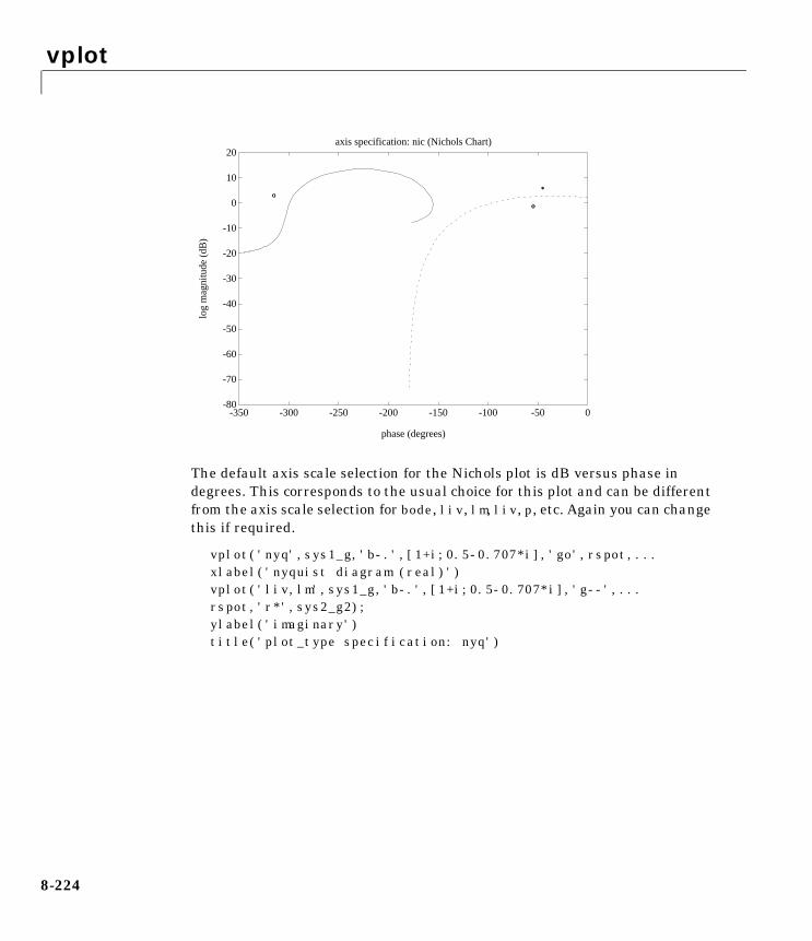
vplot
The default axis scale selection for the Nichols plot is dB versus phase indegrees. This corresponds to the usual choice for this plot and can be differentfrom the axis scale selection for bode, liv, lm, liv, p, etc. Again you can changethis if required.
vplot('nyq',sys1_g,'b-.',[1+i;0.5-0.707*i],'go',rspot,... xlabel('nyquist diagram (real)') vplot('liv,lm',sys1_g,'b-.',[1+i;0.5-0.707*i],'g--',... rspot,'r*',sys2_g2);ylabel('imaginary') title('plot_type specification: nyq')
-80
-70
-60
-50
-40
-30
-20
-10
0
10
20
-350 -300 -250 -200 -150 -100 -50 0
oo
oo
**
phase (degrees)
log
mag
nitu
de (
dB)
axis specification: nic (Nichols Chart)
8-224

vplot
See Also plot
-2
-1
0
1
2
3
4
5
-5 -4 -3 -2 -1 0 1 2
oo
oo
**
nyquist diagram (real)
imag
inar
y
axis specification: nyq
8-225

vpoly, vroots
8vpoly, vrootsPurpose Find coefficients and roots of a characteristic polynomial from a CONSTANTor VARYING matrix
Syntax matout = vpoly(matin) vecout = vpoly(vecin) vecout = vroots(vecin)
Description vpoly forms an n + 1 element VARYING row vector whose elements form thecoefficients of the characteristic polynomial, det(sI – matin(i)), if matin is ann × n VARYING matrix. The coefficients are ordered in descending powers of s.If the input is a column vector vecin containing the roots of a polynomial,vpoly(vecin) returns a VARYING row vector whose elements are thecoefficients of the corresponding characteristic polynomial.
vroots returns as a VARYING column vector vecout whose elements are theroots of the polynomial at each independent variable, if vecin is a VARYINGrow vector containing the coefficients of a polynomial. vpoly and vroots areidentical to the MATLAB poly and roots commands, but also work onVARYING matrices.
Examples Given a 3 × 3 VARYING matrix, find the characteristic polynomial and itsroots. Compare this to finding the eigenvalues of the input matrix via veig.
see(matin)3 rows 3 columnsiv = 0.11 2 34 5 67 8 9iv = 0.410 11 1213 14 1516 17 18matout = vpoly(matin);see(matout)1 row 4 columnsiv = 0.1l.0000e+00 –1.5000e+01 –1.8000e+01 –1.4483e–14iv = 0.4l.0000e+00 –4.2000e+01 –1.8000e+01 1.2818e–14
8-226

vpoly, vroots
vecout = vroots(matout);see(vecout)3 rows 1 columniv = 0.1 1.6117e+01–1.1168e+00–8.0463e–16
iv = 0.4 4.2424e+01–4.2429e–017.1212e–16evals = veig(matin);see(evals)3 rows 1 column
iv = 0.1 1.6117e+01–1.1168e+00–8.0463e–16iv = 0.4 4.2424e+01–4.2429e–01 7.1212e–16
Algorithm vpoly and vroots call the MATLAB poly and roots commands.
See Also eig, poly, roots, veig
8-227

vsvd, vrho, vschur
8vsvd, vrho, vschurPurpose Perform a singular value decomposition, spectral radius and Schurdecomposition of a CONSTANT or VARYING matrix
Syntax s = vsvd(matin) [u,s,v] = vsvd(matin) out = vrho(matin) t = vschur(matin) [u,t] = vschur(matin)
Description vsvd performs a singular value decomposition on a VARYING matrix. It isidentical to MATLAB’s svd routine, and will work on CONSTANT matrices aswell. If there is one output argument, the output is a VARYING matrix withthe singular values of matin at each point. If there are three output arguments,[u,s,v], then u is a VARYING matrix with the left singular vectors, s is aVARYING matrix with the singular values, and v is a VARYING matrix withthe right singular vectors.
vrho finds the spectral radius, max(abs(eig(xtracti(matin,i)))), at eachindependent variable of a VARYING matrix.
vschur computes the Schur form of a VARYING matrix for each independentvariable. It is identical to the MATLAB schur command, but also works onVARYING matrices. Given two output arguments, vschur returns twoVARYING matrices u and t. t corresponds to the Schur form matrix and u is aVARYING unitary matrix such that
matin = mmult(u,t,vcjt(u))
Examples Construct a random VARYING matrix and find its singular values.
see(matin)2 rows 2 columns
iv = 0.10.93040.52690.84620.0920iv = 0.40.65390.70120.41600.9103[u,s,v] = vsvd(matin);
8-228

vsvd, vrho, vschur
see(u)2 rows 2 columnsiv = 0.10.7884 0.61520.6152 –0.7884
iv = 0.40.6909 –0.72290.7229 0.6909see(s)
iv = 0.11.3400 0.2689
iv = 0.41.3681 0.2219see(v)2 rows 2 columns
iv = 0.10.9359 –0.35220.3522 0.9359
iv = 0.40.5501 –0.83510.8351 0.5501
Algorithm vrho, vschur, and vsvd call the MATLAB commands svd, eig, and schur
See Also eig, hess, pkvnorm, mu, qz, schur, svd, veig, vnorm
8-229

vzoom
8vzoomPurpose Freeze plot axes by clicking mouse twice in plot window
Syntax vzoom('axis')
Description vzoom uses the MATLAB functions ginput and axis to freeze the axes byclicking the mouse twice in the plot window that defines minimum andmaximum values for x and y. The clicking may be done in any order.
The axis argument specifies the type of graph, and can select between thevarious logarithmic or linear graph types, just as in vplot. Unlike vplot, theaxis argument is not optional. The axis specification choices are:
Note that the axis specification is the same as for vplot, with the addition ofthe last four possibilities. The function is not defined for 'bode'.
Examples The command vzoom('liv,m') would be equivalent to
[x,y] = ginput(2); axis([log10([min(x) max(x)]) min(y) max(y)]);
An example of the use of vzoom is
tf = frsp(nd2sys([ 1 .1],[.1 1]),logspace(–2,2,100)); vplot('nic',tf); vzoom('nic'); vplot('nic',tf); axis;
'iv,d', 'iv,m','iv,p' decimal, magnitude, or phase vs. independentvariable
'liv,d', 'liv,m','liv,p' decimal, magnitude, or phase vs.
'iv,lm''liv,lm'
log(magnitude) vs. independent variablelog(magnitude) vs. log(independent variable)
'ri', 'nyq' real vs. imaginary (parametrized byindependent variable)
'nic' Nichols chart
'ss' standard decimal
'll' log-log
'ls' semilogx
'sl' semilogy
8-230

vzoom
See Also axis, ginput, vplot
8-231

8wsguiPurpose A graphical user interface for the MATLAB workspace
Syntax wsgui
Description wsgui is a graphical user interface (GUI) for the MATLAB workspace. It allowsyou to view, delete, and save variables in the workspace, drag these variablesto other µ-Tools GUIs, dkitgui and simgui, drop boxes, and export variablesfrom the µ-Tools GUI interfaces to the MATLAB workspace.
The wsgui Workspace Manager window appears as shown on the followingpage.
Each time Refresh Variables is pressed, the MATLAB command who isexecuted, and minfo is run to determine the variable type and dimension. Thisinformation is displayed in the main scrollable table. The date and time of thelast refresh are displayed below the button.
8-232
wsgui
The scrollable table can be moved up/down one page by pressing above/belowthe slider. Pressing the arrows at the end of the slider moves the table one line.
A filter is used to make viewing of a reduced number of selections easy. ThePrefix, Suffix and matrix type filters are on the bottom of the scrollabletable. The matrix type filter is a pop-up menu to the right of Suffix. TheCustom filter, which is shown if * is pressed, allows you to create a morecomplicated selection criteria. Press the pushbutton marked with an *; thispushbutton is to the right of the pop-up menu, to switch to the custom filter. Adetailed description of wsgui is provided in the “Workspace User Interface Tool:wsgui” section in Chapter 6.
Examples An example of using wsgui is shown in the “Workspace User Interface Tool:wsgui” section in Chapter 6.
See Also clear, save, who
8-233

wcperf
8wcperfPurpose Computes upper and lower bounds for the worst-case gain of a linear systemsubjected to structured, bounded, LFT perturbations. Also computesworst-case structured perturbation of a specified H∞
Syntax [deltawc,lowbnd,uppbnd] = wcperf(Mg,uncblk,alpha,npts);
Description The command wcperf is associated with the block diagram
where ∆ has block structure as defined by ∆, which is described via the matrixuncblk. The worst-case performance curve, ƒ(α), is defined as
Both lower and upper bounds for ƒ are returned as VARYING matrices inlowbnd and uppbnd. Each VARYING matrix is guaranteed to have at least nptsvalues of the independent variable α, spread uniformly between 0 and thestability limit.
The first output argument, delta_wc, is the “worst-case” perturbation from ∆with norm equal to the value of alpha. delta_wc has the block-diagonalstructure associated with uncblk, and causes the LFT FU (M,∆wc) to have normequal to the value of lowbnd associated with the independent variable valueα = alpha.
See Also dypert, mu
f α( ) := max FU M ∆,( ) ∞∆ $∆,∈ maxwσ ∆ jω( )( )ðα
8-234
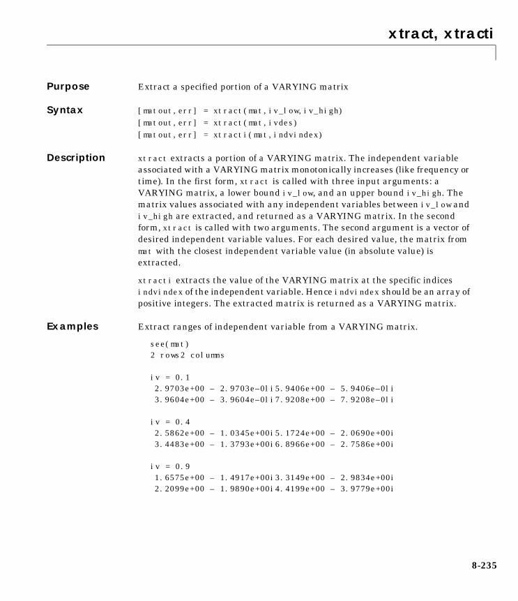
xtract, xtracti
8xtract, xtractiPurpose Extract a specified portion of a VARYING matrix
Syntax [matout,err] = xtract(mat,iv_low,iv_high) [matout,err] = xtract(mat,ivdes) [matout,err] = xtracti(mat,indvindex)
Description xtract extracts a portion of a VARYING matrix. The independent variableassociated with a VARYING matrix monotonically increases (like frequency ortime). In the first form, xtract is called with three input arguments: aVARYING matrix, a lower bound iv_low, and an upper bound iv_high. Thematrix values associated with any independent variables between iv_low andiv_high are extracted, and returned as a VARYING matrix. In the secondform, xtract is called with two arguments. The second argument is a vector ofdesired independent variable values. For each desired value, the matrix frommat with the closest independent variable value (in absolute value) isextracted.
xtracti extracts the value of the VARYING matrix at the specific indicesindvindex of the independent variable. Hence indvindex should be an array ofpositive integers. The extracted matrix is returned as a VARYING matrix.
Examples Extract ranges of independent variable from a VARYING matrix.
see(mat)2 rows2 columns
iv = 0.12.9703e+00 – 2.9703e–0li5.9406e+00 – 5.9406e–0li3.9604e+00 – 3.9604e–0li7.9208e+00 – 7.9208e–0li
iv = 0.42.5862e+00 – 1.0345e+00i5.1724e+00 – 2.0690e+00i3.4483e+00 – 1.3793e+00i6.8966e+00 – 2.7586e+00i
iv = 0.91.6575e+00 – 1.4917e+00i3.3149e+00 – 2.9834e+00i2.2099e+00 – 1.9890e+00i4.4199e+00 – 3.9779e+00i
8-235

xtract, xtracti
matl = xtract(mat,.3,.8);see(matl)2 rows2 columns
iv = 0.42.5862e+00 – 1.0345e+00i5.1724e+00 – 2.0690e+00i3.4483e+00 – 1.3793e+00i6.8966e+00 – 2.7586e+00i
matl = xtracti(mat,2);see(matl)2 rows2 columns
iv = 0.42.5862e+00 – 1.0345e+00i5.1724e+00 – 2.0690e+00i3.4483e+00 – 1.3793e+00i6.8966e+00 – 2.7586e+00i
See Also sel, var2con, vpck, vunpck, vfind
8-236

Index
Aabv 8-19
example 2-12
Bblknorm 8-22
HIMAT example 7-98
Ccf2sys 8-129
HIMAT example 7-127cjt 8-24cmmusyn 8-27CONSTANT matrices 2-8
diagram 2-14control design
spinning satellite example 6-14cos_tr 8-28crand 8-30crandn 8-30csord 8-32
Ddata structures 2-3daug 8-19Destabilizing perturbations
constructing 7-41dhfnorm 8-34dhfnormBody text>
example 3-15dhfsyn 8-35
example 3-46dhinfsyn
example 3-43
D-K IterationHIMAT dkit example 7-100HIMAT example 7-85
D-K iteration 5-3commands 5-13discussion 5-14D-scalings 5-7full D-scaling 5-10holding Dfixed 5-9holding Kfixed 5-10µ upper bound 5-6problem formulation 5-3
D-K iteration user interface 6-19auto iteration 6-36D-K iteration 6-30example 6-19main window 6-20options 6-38parameter window 6-26setup window 6-20
dkit 8-38HIMAT example 7-100HIMAT setup file 7-102
dkitgui 6-2, 6-18, 8-44unstable example 7-28
dragging and dropping icons 6-66dkitgui 6-66example 6-68simgui 6-66wsgui 6-66
drawmag 8-46D-scalings
automatic prefitting 7-109, 8-42dtrsp 8-181
example 2-26
I-1

Index
I-2
dypert 8-48constructing perturbations 7-41
Eemargin 8-129
FF–14 lateral-directional control design 7-132fft
example 2-27fitmag 8-51fitmaglp 8-51fitsys 8-55frsp 8-56
example 2-20
Ggain and phase margins 7-3gap 8-61genmu 8-63genphase 8-51getiv 8-65GUI
D-K iteration tool 6-19D-K workspace tool 6-2LFT time simulation tool 6-41
HH∞ Control 3-1
commands 3-16design example 3-18discrete-time 3-43full control 3-31
full information 3-31generalizations 3-41history 3-22loop shaping 3-52norm calculation 3-41notation 3-23output feedback 3-36performance objectives 3-10problem definition 3-25sampled data 3-43theory 3-20
H∞ loop shapingHIMAT example 7-121reference signal 7-128
h2norm 8-67example 3-14
h2syn 8-69hankmr 8-172
example 3-55HIMAT design example 7-75hinffi 8-72hinfnorm 8-67
example 3-14hinfsyn 8-77
example 3-17HIMAT example 7-89shuttle example 7-55
hinfsyne 8-82example 3-17
Iifft
example 2-27indvcmp 8-85

Index
LLFT time simulation user interface 6-40
continuous-time 6-61discrete-time 6-61example 6-40integration step size 6-55loading and saving 6-59main window 6-41parameter window 6-55plot titles 6-49plots and line type table 6-46printing 6-59sampled data 6-62
Linear Fractional Transformations (LFTs) 4-3loop shaping 7-86
Mmadd 8-87
example 2-11magfit 8-51massign 8-90mfilter 8-93minfo 8-95
example 2-4minv 8-97mmult 8-99
example 2-11model reduction 3-55
balanced realizations 3-59Hankel-norm 3-57relative error 3-66weighted 3-65
mprintf 8-102mscl 8-105msf 8-103msfbatch 8-103
msub 8-87example 2-11
muexample 4-31mixed perturbations 4-64
mu 8-109HIMAT example 7-93MIMO example 7-38
muftbtch 8-116multivariable margins 7-7musynfit 8-116musynflp 8-116muunwrap 8-109
Nncfsyn 8-129
HIMAT example 7-123nd2sys 8-126negangle 8-128nominal performance 7-83
HIMAT example 7-87unstable example 7-15
norms 3-3commands 3-14performance 3-5
nugap 8-61HIMAT example 7-127
Pparametric uncertainty 4-5pck 8-132performance objectives
F-14 example 7-134unstable example 7-15
I-3

Index
I-4
pkvnorm 8-135hinfnorm 3-14
plot 2-15pss2sys 8-132
example 2-5
Rrandel 8-109reordsys 8-151representing uncertainty 4-3ric_eig 8-137ric_schr 8-139Riccati operator 3-28rifd 8-140
example 2-5robust control design 5-2robust performance 4-73, 7-83
F-14 example 7-146HIMAT example 7-85, 7-93shuttle example 7-64unstable example 7-19
robust stability 4-31, 4-71
Ssamhld 8-141sbs 8-19
example 2-12sclin 8-105scliv 8-143sclout 8-105sdecomp 8-162
example 3-66sdhfnorm 8-144
example 3-47
sdhfsyn 8-146example 3-47
sdtrsp 8-181see 8-149seeiv 8-149
example 2-7seesys 8-150sel 8-151
example 2-9sensitivity 7-80sfrwtbal 8-162sfrwtbld 8-162
example 3-65siggen 8-154
example 2-23simgui 8-159
shuttle example 7-68sin_tr 8-28sisorat 8-48
constructing perturbations 7-41sncfbal 8-162
HIMAT example 7-126sortiv 8-65
example 2-8space shuttle
time simulations example 7-67space shuttle FCS analysis 7-44spectrum
example 2-30spoles 8-161
example 2-5srelbal 8-162
example 3-66sresid 8-166
example 2-9starp 8-168
example 7-8

Index
statecc 8-170state-space uncertainty 4-20step_tr 8-28strans 8-170
example 3-55structured singular value (µ)
block structure 4-56bounds 4-54complex µ exercise 4-56complex µ theory 4-50D-scales 4-54D-scalings 4-58frequency domain 4-70generalized µ 4-81mixed µ exercise 4-64mixed µ theory 4-61mixed upper bound 4-61perturbations 4-59real and complex blocks 4-61real blocks 4-74robust performance 4-73robust stability 4-71theory 4-49
strunc 8-166example 2-9
sys2pss 8-132example 2-5
sysbal 8-172example 2-9
sysic 8-176description 2-34F-14 example 7-142HIMAT example 2-38, 7-83unstable example 7-15
sysrand 8-30example 2-5
SYSTEM matrices 2-3
diagram 2-14szeros 8-180
example 2-5
Ttackon 8-65transp 8-24trsp 8-181
example 2-22tustin 8-190
example 2-22two tank example 7-151
closed-loop analysis 7-179closed-loop experiments 7-161linearized model 7-166nonlinear model 7-152open-loop experiments 7-158problem formulation 7-165
two tank experimentuncertainty models 7-168
Uuncertainty
aero coefficients 7-53shuttle example 7-45
uncertainty modelF-14 example 7-135HIMAT 7-78unstable example 7-15
unpck 8-132example 2-5
unstable example 7-15unum 8-194unwrapp 8-109
I-5

Index
I-6
Vvabs 8-195var2con 8-214
example 2-10VARYING Matrices
diagram 2-14VARYING matrices 2-6varyrand 8-30vceil 8-195vcjt 8-24vdcmate 8-211
example 2-27vdet 8-197vdiag 8-197vebe 8-199
example 2-18veig 8-201veval 8-204
example 2-18vexpm 8-197vfft 8-206
example 2-25, 2-27vfind 8-210vfloor 8-195vifft 8-206
example 2-27vimag 8-195vinterp 8-211
example 2-25vinv 8-97vldiv 8-213vnorm 8-135
example 3-15
vpck 8-214example 2-7
vpinv 8-213vplot 2-15, 8-216
example 2-15vpoly 8-222vrcond 8-197vrdiv 8-213vreal 8-195vrho 8-224vroots 8-222vschur 8-224vspect 8-206
example 2-30vsvd 8-224vtp 8-24vunpck 8-214
example 2-7vzoom 8-226
Wwcperf 8-229workspace user interface 6-3
clearing and saving 6-9customize 6-7
workspace user interface filter 6-4font and lines 6-10
worst-case performanceunstable example 7-146
worst-case perturbationsshuttle example 7-65
wsgui 8-227
Index
Xxnum 8-194xtract 8-230
example 2-9xtracti 8-230
example 2-10
Yynum 8-194
Zzp2sys 8-126
I-7

Index
I-8