_, ,%A;SAContractor Report 170400 it

. T

---= (NASA-CR-170_00) ;_N INVP.STIGATION OF THE N83-26760': INTERNAL &ND EKTERNAL AERODYNANICS OF CATTLE: TRUCKS Final Report (Kansas Univ, Center

. for Research, Inc.) _7 p HC A05/NP A0! ,nclasCSCL !3F G3/R5 03856

=_ An Investigation of the Intemal andExternalAerodynamicsof CattleTrucks

(lllllk,

V!ncent U. Muirhead ,_

", Grant NAG4-8.. • May 1983

: r_=;l',-,,i Aeronauticsand _':__eT':, Space Administration __._:/_-

1983018489

https://ntrs.nasa.gov/search.jsp?R=19830018489 2019-07-09T23:50:06+00:00Z

,=

... NA._;A t',,Itl,h'l*, th'p_,! 1/11.11111

.

.L,

_.

-L.. An Investigationof the Intemaland....' ExternalAerodynamics of Cattle Tracks

i "',; _.'m_'_rlttl Mtlllhl_dld. UnIV¢_ISlII el kllll,_118 COIlttll fOI Research. Ine.. Lawrence.Kansn,q

= ;i -

k ':".p

g _"

-':-:.;; _111¢1,_;ttIiSIi_IIL'|I (=3lilt|Ill

.... I_v_'d_m I Ihlht llt_,,_t)dlv,,'hI_l_'lllI_";,; and lh,_

i .-,:5. ,.

': Niltlltlhll Al_lktltdltlth'I_ ltllI| _,_.,_,._._".'/

'', Ames ROllllCh Center I,I,8.llo|ttlltlllOltI k_lAgv=_'utluve

"!, Ilv_d_,n t Ihlht Ilt_,_l_,|Ich t _l,'llll_ Aglll,;ul|ult_ |tO,qt_illl_It RI_IVlt'I_ 1,l,qa, ,I [I I_tm¢_, Llkltlh_m_/,tO,tt_t ittq_lltt,';. L_,lllhtlllllt 1 i t , ,

_, i d,

1983018489-TSA03

ZTABL_ OF COh_NTS

P_S

TASLE OF CONT_TSeooeoeeeoeeoeeeee.**** ...... *eeee*eeoteeeeeeeeeoeoe i

_IST OF S_EOLS ............ **, .... ,0, ......... , ....... , ..... 00****** ii

_ LIST OF FIGURESoo,.**********,,,**,*********,o,,,ooeoooooooooe,,**** iV

LIST OF TABLES..,....,.. ..... .. ..... , ........ , ...... ,,..,,.,,,,.,,., Vii

•_ AC_OW_EDG_4_TS.° .... °.0 ...... °°.°o.o.°°.°°.*..oooooo°°...°°,.°°.°.Vi££

, S_I_Ry ...... °°.0 ......... 0°°° ...... e .... °o°_. ........ 0° ..... °°o°oe° iX

: 1. INTRODUCTION.....° ...... , ..... .0 ........ ....0.0.0,,000... ...... 1

20 APPARATUS AND PROCEDURE ......... 00o ..... o ........ . .... . ........ 3i,

2.1 Nodels ..... . ...... ., ...... , ........ . .... ,...**,...** ...... 3

: 2.2 _untlng ........ .......,.,.......... .... ...,, .... . ........ 4

: 2.3 Te8ts.**...**......,.,..,.****...**.,.,...,..........,.,.. S

3. RESULTS AND DISCUSSION.,. ............ . ........... , ...... . ...... S

:' 3.1 Internal Trailer Airflow Patterns..... .... ,.,....... ...... 5

3,2 Internal Tcailer _irflow Speeds...... ....... ,..,.... ...... 8

3.3 _elttng Times for I_e Cubes in Trailer ...... , ...... . .... .. 11

3.4 Drag Coefficients and Power Required ............... . .... .. 11

: 3.5 Side Force Coe_ficlents ............ , ........ .., .... ., ..... 13

3._ Lift and _k_ment Coefficients ....... . ........ . ...... , ...... 14

t 4. CONCLLISIONS AND RECOMMENDATIONS ......... •........ .° ..... ..... .. 14

_. REFERENCES .............. , .... ,***, .... .**.,,.o°..°.°..°°,°o°o.. 16

6. _IGURES AND TABLES ...... * .... ..**.*....*.***..*..* ..... ... ..... 17

"-_+ 7. APPENDIX ....... ..... .... ,......*.,. .... .,*.. ..... , ...... ....... 75

:r

+: iI;

i,1 + : + +_ -=++- _+ _.... + + : " _ + 22+2 ++ 2; 2+'_+ ?+i ? +21+_225_+_+22+_+ + .++ 2+++'_:-"+_]J!_+" : :+

' .....' + -' .... 1 4 TSA0983018 +89" -: -4k n

::_ ORIGINAL PAGE IgOF_POOR QUALITY

LIST OF SYMBOLSi e ,

:: _ Definition

- _: A Projected model frontal area (less wheels) on a plane

_. perpendicular to the centerline of vehicle, .0915 sq m1.986 sq re)

;i a

;,. At) Base area at the aft end of livestock trailer

Abv Total area of vent openings in base of trailer

'" As Total side area of trailer (one side)

• "",:,_ Asv Total arJa of slotted openings on one side of trailer

6,:" Ai Total ar_a of ram-air inlet or NACA submergsd inlets,

normal to longitudinal axis of model

Totalareaof=.ifoldductingope.lngsatthe rontwall.._"-:- of the livestock compartment

_. CD Coefficient of drag, D/qA

• /l

_..._ CL Coefficient of llft, L/qA

._. CM Coefficient of pitching moment, PM/qAc

""' Cy Coefficient of side force, SF/qA

:'! C£ Coefficient of rolling moment, RM/qAc

,:'_ _ Coefficient of yawing moment, YM/qAc

,,_" CDx Coefeicient of drag, configuration X

_:° Cp Coefflcient of static pressure, (P - PA)/q

o.,", c Reference length (vehicle length for CM)

':" (vehicle width for C£, CN)

D Drag (vehicle axis)

"." De Equivalent diameter,

=°i";. L Lift (vehicle axis) .!o.:.: P Powe r •

:: '- PA Atmospheric pressure

:",- il

i983018489-TSA05

i

i" ,tinltlo.

i t, _waL static ptossure

PH Pitching moment (vehicle axis)

q True dynamic pressure in wind tunnel test section, 1/2pY 2

RM Rolling moment (vehicle axis)

RN Reynolds number (based on equivalent diameter, _-_ )

i, SF Side force (vehlcle axis)

-t V Relative wind speed = Wind tunnel airspeed

V 1 Vehicle speed

•'; V2 Side wind component

W True wind speed

YM Yawing moment (vehicle axis)

8 Wind angle relative to vehicle path

p Air density

M Air viscosity

Yaw angle = Relative wind angle

Ill

1983018489-/_/...kUO

LIST OF FIGURES

Number Titlem

2.1.1 Photograph of ba_eltne wind tunnel model,conflfuration 1........ .... .......,.................... 18

2.1.2 Baseline wind tunnel model, configuration 1............ 19

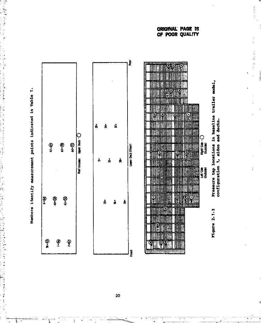
2.1.3 Pressure tap locations in baseline _railer model,

configuration I, sides and decks................. ...... 20

2.1.4 Pressure tap locations in baseline trailer _odel,

configuration 1, front and rear. .... .. ...... ...... ..... 21

2.1.5 Tuft 1ocatlons in trailer models, 2, S, and 6.......... 22

2.1.6 &Irepeed measurement locations in trailermodels 2, 5, and 6........... •....... •.... ....... ...... 23

2.1.7 Zce cube locations in trailer models 2, 5, and 6

for ice cube melting tests..0.0....... .... o...... ...... 24

2.1.8 Side view of streamline wind tunnel models. .... ..0 ..... 25

2.1.9 Forward streamlining, full scale, as inreference 8, 10, and 13.... ........... .... ......... .... 26

2.1.10 Photograph of forward streamlining and ram air inlet

on configuration 5. .......... • ....... .... ....... • ...... 27

2.1.11 Ram air inlet and ductlng design applied to

configuration 5.......... .... .... ........... ..... ...... 28

2.1.12 NACA submerged inlet and ductlng design appliedto configuration 6. ........ .., ..... ... ..... ............ 29

2.1.13 Cattle simulation design ................ *''' .... ''''''" _O

2.1.14 Model configuration chart .... • .... ...................... 31

2.1.15 Important Phyeloal Proportions for models ....... ..., .... 32

3.1.1 Air flow in trailer _ - 00, configuration I,

isometric view indicating air flow direction only .... .. 33

3.1.2 Air flow in trailer, _ - 00, configuration I,

upper and rear decks.... ..... ........ ....... ........... 34

3.1.3 Air flow in trailer, _ - 00, configuration I,lower deck ....... . ..... ..... .... ............ .... . ...... 35

1

3.1.4 FAr _low in trailer, _ = 150 configuration 1, 1isometric view indicating air flow direction on1¥...... 36

iv

4

1983018489-TSA07

3.1.5 air flow in trailer, _ _ 150 , configuration 1,upper and rear decks ................................... 37

3.1.6 Air flow in trailer, _p= 150 , configuration 1,lower deck ............................................. 38

3.1.7 Photograph of tufts in trailer, configuration 1," _ = 0v ......................... -- . ................... • 39

3.1.8 Fir flow in trailer, _ = 0O, configuration 2,upper deck above cattle ................................ 40

3.1.9 Fir flow in trailer, _ = 0O, configuration 2,upper _eck below cattle ................................ 41

3.1.10 Fir flow in trailer, _ = 0O, configuration 2,lower and rear decks above cattle ...................... 42

3.1.11 Air flow in trailer, $ = 00, configuration 2,lower and rear decks below cattle ...................... 43

3.1.12 Fir flow in trailer, _ = 150 , configuration 2,upper deck above cattle ................................ 44

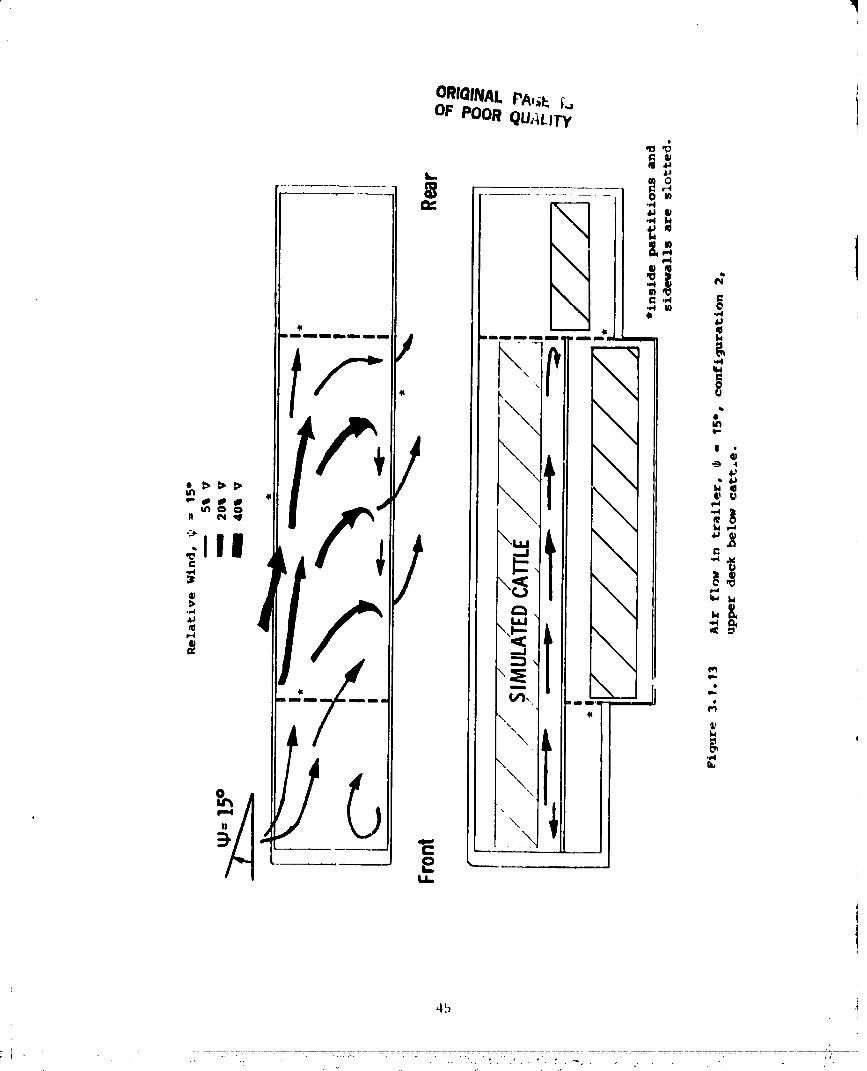
3.1.13 air flow in trailer, 9 = 15O, configuration 2,

upper deck below cattle ................................ 45

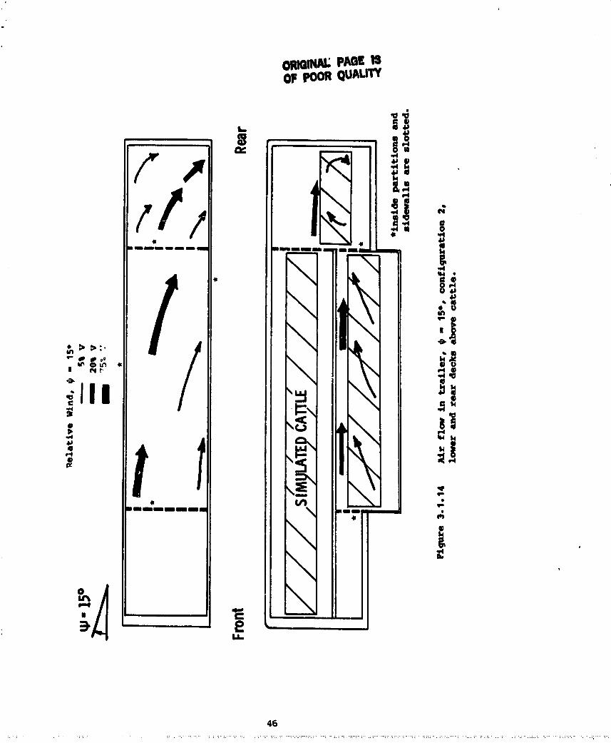
3.1.14 Air flow in trailer, _ = 150 , configuration 2,lower and rear decks above cattle ...................... 46

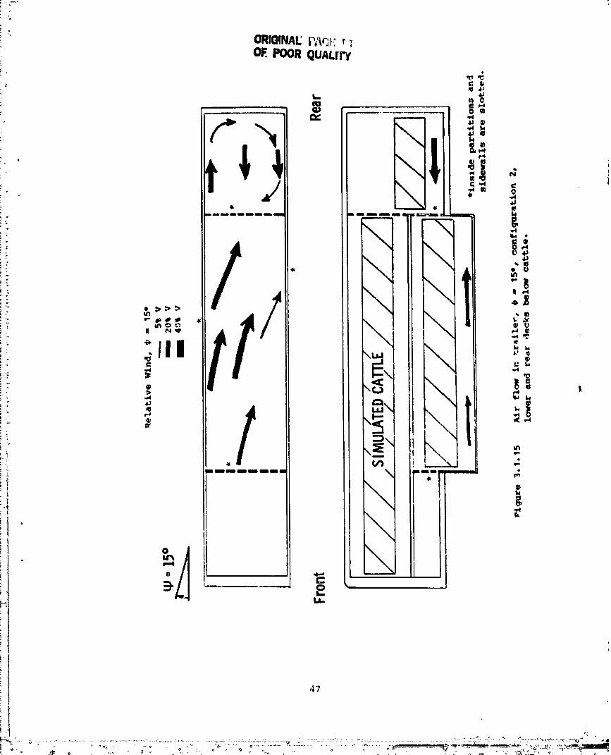
3.1.15 Air flow in trailer, _ = 150 , configuration 2,lower and rear decks below cattle ...................... 47

3.1.16 Air flow in trailer, _ = 00, configuration 5........... 48

3.1.17 "%r flow in trailer, _ = 150 , configuration 5.......... 49

3.1.18 Air flow in trailer, _ = 00, configuration 6.......... 50

, 3.1.19 Air flow in trailer, _ = 150, configuration 6.......... 51

3.4.1 ReFnolds number effect on drag coefficient,

. configuration 1........................................ 52

3.4.2 Effect of relative wind angle on drag coefficient,

configuration I........................................ 53

3.4.3 Effect of relative wind allgle on drag coefficient,

configuration 3........................................ 54

3.4.4 Effect of relative wind angle on drag coefficient,

configuration 4........................................ 55

V

4

.................................. i 983018489-TSA08

3.4.5 _o_arieon of _ag coeff_ciente_ conflguratlone le3o 40.... ........ 0.... ............. °..° ........ ° ....... S6

3.4.6 Power required to overcome aerodynamic drag_configurations 1, 3, 4 ...... .. .... ... ........ ,.... ..... 57

3.5.1 Reynolds number effect on s£de force coeffic£ent, , _conf£guration 1...... . ...... . ................ . ......... 58 1

3.5.2 Effect of relative wind angle on side force !coefficiente configuration 1........................... 59

3.5.3 Comparison of side force coefficients0 Configura-tion 1, 3, 4 ........................................... 60

3.6.1 Effect of relative wind angle on lift coefficients,

Configuration 1 ..................................... ... 61

3.6.2 Comparison o5 lift coefficients, Configurations10 3e 4 ..................... . ................ • ......... 62

vt

" " 1983018489-TSA09

LIST OF TABLES

._he: TitZe

I Coefficients of Static Preesure, Conflqur=tion 1....... 63

II Internal Air Flow Speeds, Configuration 2 .............. 67

. Ill Internal Air Flow Speeds, Configuration 5 .............. 68

IV Internal Air Flow Speeds, Configuration 6 .............. 69

V Internal Air Flow Volumes for Models ................... 70

VI Melting Times for Ice Cubes from Internal Air

Flow, Configuration 2.................................. 71

VII Meltings Times for Ice Cubes from Internal Air

Flow, Configuration 5.................................. 71

VIII Melting Times for Ice Cubes from Internal Air

Flow, Configuration 6.................................. 72

IX Drag Coefficients ...................................... 72

X Potential Fuel and Economic Savings of Nodigied

Vehicles Relative to Configurations I and 2............ 73

XI Side Force Coefficients, _ = 7x105 .................... 73

XII Lift Coefficients, _ = 7xI05 .......................... 73

XIII Pitching Moment Coefficients, RN - 7x10 5 ............... 74

XIV Rolling Moment Coefficients, _ = 7xi05 ................ 74

XV Yawing Moment Coefficients, _= 7x10 5 ................. 74

vii

1983018489-TSA10

., ACKNOI_._gI_GMEt,1TS,

• The a4viee and eom_sntm of Mr. Edwin _ltzmane NAB& _yden Flight

Re_enrch Pacility, are gratefully acknowledged. The wind tunnel testinq

. and data reduction were ¢ondoted by the following students in tho

: Department of Aerospace Zngtneeringe University of Xansas: ,

Oa¥ Brandonw Graduate student

.... Carlos Blacklock, Undergraduate student

,.. Michael 0wings, UndergTaduate student,,i;.... Sheryl 8cotte Undergraduate student

T

._

g

.;

'7

('

,_ viii

l _:_0 0 U / 0"1" (.) ,_ / _,.)/-_ / /

i

1.0 INTflODIIC'PZ_N i

The environmental conditions which extmt during th_ trannit of

liva_to_k greatly effect the shrinkage which the animml_ undergo and the

qu_ try of the meat _hen slaughtered. Rlthough the problnma _oelat_d

with the mass transit of Iiveotouk are similar to thooo anooeta_ed with

the transit of humans, the problems encountered _rith livestock are much 1

4greater because of "the greater heat production pot animal, the propor-

tion of latent heat (evaporative) to the total heat, hi,her an£mal

loading density and management factors. "1 large volumes of heat and

metabolic byproducts must be removed.1-5

Some of the factors which effect shrinkage and meat quality are,

1. Air temperature in hauler

2. Air movement in hauler

3. Humidity in hauler

4. Wind chill in hauler

5. Distance and time in transit

6. Exposure to dust, smoke, snow, rain, hail, wind

7. Degree of excitement in transit

8. Space per animal

9. Initial body weight

10. Kind of animal, species

Under good conditions the shrinkage may vary from I% to 8% in

present vehicles. Freezing rain and low temperatures, or high tempera-

tures and humidity can be deadly. The effect of long-term preslaughter

stress such as occurs in transit depletes muscle glycogene. This

results in dryer meat with a darker color and a higher pH. 2

Specia£ efforts have been made to control the environment for

. dlsease-exposed cattle during transit 5 and in the air shipment of

livestock. I Efforts have been made (by J. H. Thorne & Sons, Ltd.,

• Shropehlre, England, and in Denmark) to improve air flow in haulers for

pigs. A venting system for a double deck standard truck was patented by

H. L. _Gan. 6 Recently a patent has been granted for a streamline

livestock hauler concept with a venting system to improve Internal flow

condltlons. 7

1

1

1983018489-TSA12

I_rtnq the pa_t decade considerable research haa been conduc_e4 to

r_du_ the aerodynamic drag on tractor trailer vehlcla_, smaller two-

axl_ trucks, recr@a_ion vehicles an4 automobiles. _nese vehicles have

been aloaed van type _arqo vehtcleo, without slde ventlng _uch _s

_ livestock trucks conventlonallF here, This research has shown that a

nlgnlflcant reduction in aerodynamlc drag can be achieved by the proper

: streaminingl 8"13 thereby reducing fuel consumption considerably.

_ost vehicles used to transport livestock have numerous small

openings along the sides for ventilation and they usually have solid,

i.e., unvented, walls at the front and rear of the livestock

': compartment. This arrangement generally increases the aerodynamic drag

and, of more importance, presents an uncontrolled environment in the

cargo compartment, i.e., poor ventilation for the annals. This°

environment subjects the animals to:

- 1. v_rious wide ranging and uncontrolled localized air flow

speeds and directions

: 2. various and uncontrolled amounts of exhaust fumes, dust

. particles, rain, sleet and snow

- 3. local pooling of poor quality air due to poor flushing:r

capability4. local severe turbulence conditions due to vortices

5. a variety of uncontrolled temperatures and hu_tdity

'_ conditions.

' Thus, it would appear that by the proper aerodynemic design of the

vehicle the environment for the animals can be greatly improved and the

aerodynamic drag reduced.

Wind tunnel tests have been conducted at the University of Kansas

i : on a one-tenth scale model of a conventional trachor trailer cattle

hauler (empty) to determine the air flow patterns through the trailer

and the drag of the vehicle. These results were used as a baseline for

_ c_mparison with results of tests on subsequent _odificatione which were

made to the baseline vehicle. The modif_catione reported herein are:

1. baseline model with a full loading of s_ulated cattle,

2. baseline model with smooth sides,

" 3. baseline model with smooth sides and streamlining,

i"i

1983018489-TSA13

4. streamline model with two forebody modifications and vented

bane rngion intended to provide improved ventilation in the

Ltvaatoak tratler (and had the nmooth alden aa in item 1,

4bore ),

2.0 pp T.s2.1 Models

The baseline wind tunnel mo]e_, Configuration 1, is shown in

Pigures 2.1.1 through 2.1.4. It Io a o,e-tenth scale model of a geomet-

rically representative cattle trailer and a cab-over-engine tractor.

The structural base of the model was constructed of steel and was

mounted on the wind tunnel balance with two nupport struts. The tractor

cab was constructed of fiberglass and mounted on the s_r,z_ u_l bas.

The trailer sides, top and intermediate floor were constructed fro _

Plexiglass; the front and rear ends were made of wood. Wooden " _,

were mounted on steel rods attached to the structurK .e.

The important geometric features of c_ '_ -_,oct trailer

design were closely simulated, including: ,.Jal_d external dimensions;

side panels and open slots, including a representative overall ratio of

slotted area to total side panel area and the vertical and longitudinal

distribution of the openings; vertical posts; and internal floors and

bulkheads. The wall and floor thicknesses were not scaled. The major

_eatures o_ the cab were also closely simulated, but detail_ were

omitted. Figures 2.1.5 through 2.1.7 show the location of tufts, air

speed probes and ice cube melt points in the trailer models. The

melting times of small ice cubes which were placed at these points were

used as indicators of the relative local ventilation characteristics°

The streamline tractor trailer model (without provisions for

ingesting ventilation alr) is shown in Figure 2.1.8. This is the same

basic shape, except for the "dropped" mid region o_ the trailer, as

tested in the wind tunnel and r_ported in references 8 and 13, and as

tested in full scale, references 10 and 13. Details of the forebody

geometry at full scale are shown in Figure 2.1.9.

Figures 2.1.10 and 2.1.11 show features of models having the

_orebody geometric proportions of the previous two figures confined with

ram air inlets for providing positive ventilation for the cargo compart-

3

............ 1983018489-TSA14

' ++j,

i

ment. _ co,_lgura_lon which uses the NACA submerged inlet concept is

shown An Plate 2.1 • 17.

+.i:_ Simulated cattle _re used in configurations 2, 4, 5 and 6. These" were simulated by using e_dified rectangular styrofoam blocks to

represent the cattle bodies. The blocks were notched at the top, bottom _

• 'l !" and each s_de to simulate a closely packed loading. Wooden dowls were

used to simulate the legs supportir_g the c_mulated bodies. These

_.. features are shown in Figure 2.1.13. & config_ration chart, Figure

2.1.14, shows a summary list of the mo._el configurations tested. It is

_ important to notice in figure 2.1.14 that whereas configurations 5 and 6

o_ had solid (i.e., unvented) side walls for the livestock compartment,

ii these were the only configurations having vents in the base region. &

:= listing of important inlet and exit ventilation areas is given in Figuret

; 2.1.15.

: 2.2 Mounting

o_= The models were mounted directly on two supports on the wind tunnel

balance, Figure 2.1.2, so that the wheels of the model were approximate-w"

_:_? ly .794 cm (313") above the floor of the wind tunnel. This is no_ the

=_- usual arrangement for mounting a truck model. Because of the relatively

large size of the model, with respect to the test section, there wasn't

_,"_ sufficient space for a conventional ground board. While this was a less

o_ than optimum arrangement for measuring forces, the larger model was

_. deemed to be important to enhance the internal pressure, flow direction ,P

and air speed measurements which would have been more difficult to

_ define within a smaller model.

. The flow over the model was observed from either side of the test ,

, section and from above the test section. The model could be rotated 20"

....._ in each dlreotlon from the centerllne of the wind tunnel. A nozzle to

emit neutrally bouyant helium bubbles was mounted in a traversing

•i_: mechanism upstream of the test section (the helium bubbles provided a8

i_ visual indication of flow patterns). This enabled the positioning of

_ the bubble stream at varying heights along the vehicle, varying lo_a-

:?_ tlons across the front of the vehicle and at various distances from the

°,_ tractor and/or trailer. The bubbles wore illuminated by two zenon

_" 4 i+ii I

98308489- ISBO

• .o

q,r

_Ights downstream of the models as well as flood lighting in the test

section area..

2.3 Testsm

The tests were conducted in the .91 by 1.29 meter wind tunnel at

the University of Kansas _t Reynolds numbers of 2.5 x 105 to 10.1 x 105

based upon the equivalent diameter of _he vehicle or 1.27 x 106 to 5.15 \ 1

x 106 based upon the length of the baseline model. The Reynolds number

was controlled by adjusting the wind tunnel airspeed from 40.5 to 159.5

kilometers per hour (25.2 to 99.1 mph). Tests were made at yaw (rela-

tlve wind) angles of 0°, 5°, 10° , and 15° at four different Reynolds

numbers. Force and moment data were obtained from a six-component,

_: straln-gauged balance. Pressure measurements were made by an alcohol

z monometer. A Sage Action, Inc., neutrally bouyant helium bubble system

and tufts were used to visualize the air flow inside the trailer and

: around the entire model. The bubble flow and tufts were visually

observed and manually recorded as well as photographed with a 35 m

camera.

Probes were placed inside the trailer model to measure air speeds

in each section of the trailer. Ice cubes (volume of 1.96 ml) each were

placed inside the trailer to obtain a relative melt time interval from

the air flow in configurations 2, 5 and 6. During each test one cube

was placed on the top of the trailer in quasi-free stream flow in order

to provide a reference for correlating the numerous tests.I

3.0 RESULTS AND DISCUSSION

3.1 Internal Trailer Air Flow Patterns

' 3.1.1 Baseline Model, Configuration I.

The internal air flow in the trailer oE the baseline model (without

81mulated cattle) is illustrated in Figures 3.1.1 through 3.1.7. These

illustrations are a composite of manually recorded visual observations

and photographs of both helium bubble flow and tuft patterns. Three

intensities of lines are used in Figures 3.1.2, 3.1.3, 3.1.5 and 3.1.6

Ln order to provide some understanding of the flow speeds in the

trailer. These intensities were established from the observed bubble

Flow speed, the tuft activity level and pressure measurements. The

5

1983018489 YS802

ORIG_IALPAGE ItlOF POORQUALITY

._,. pressure coefficients in Table Z (exterior and interior) were calculated

from Local static pressures measured on the surfaces of the trailer.

':.: _e air flow in the trailer was turbulent and the head losses unknown.

- Therefore, the coe_ficients do not reflect the true local airspeeds.

The coefficients were used to assist in establishing quantitativel¥ the

;: relative speed scales on each of the flow illustrations.

:: At a relative wind angle of $ m 0 O, the air flowing over the cab

and trailer entered the trailer in the forward and central region,

Pigures 3.1.2 and 3.1.3. The air entered on the right (starboard) side

and exited along the left (port) side. This was caused by a flow

it: angularlty of less than one degree and small variations from symmetry of

the cab. The highest air flow speeds and the strongest vortices

;i_ occurred in the forward portions of the upper and lower deck areas. The

-_ air flow speeds diminished in the aft regions of the trailer.

i_ At relative wind angles of $ = 50 and 10", not shown herein, and

°_ 15° Figures 3.1.4 through 3.1.6, the air entered the trailer over the

_orward half of the trailer on the right (windward) side of the trailer

and exited on the left (leeward) side. As the relative wind angle

increased, the internal air flow speeds progresslvel¥ increased in the

forward part of the trailer with the flow patterns remaining similar,

i_ _igures 3.1.4, 3.1.5 and 3.1.6. The airflow in the rear deck area of

the trailer became negligible at _ = 10 0 and _ = 150 relative wind7. angles.

:. Generally the internal flow for the empty trailer was characterized

by turbulence, vorticity and some forward flow in the upper and lower

_ deck areas. Tn the rear deck of the trailer there was very little air

i movement. Also from the general flow conditions it would appear thati n

dust• smoke particles or other impurities entering the trailer would be

: most concentrated in the forward part of the trailer. In all cases the

_: conditions which existed within the trailer varied as a function of the

_'_ relati_J wind speed and direction.

3.1.2 Baseline Model with Simulated Cattle, Configuration 2.

The internal flow in th :railer with a load of simulated cattle is

:z illustrated in Figures 3.1.8 through 3.1.15. These illustrations ware

:, ms,Is ?tom visual observations of tufts placed inside the trailer. The

v

' ° .... 9830

e .

1 18489-TSB03

l_l,_,'k.l,l,','.I_1rI,_,I|_f lllt_ _'_IIII_ l_l'_i,lll_','dllill III,II|IIl_|llllt_ll111|II ||Ill r|llN

l_._ll,_l'lltl,_I'lho ,_ml_li* 110_II_I"I II l h_ lllt¢_l'll&l f|_W¢l Wl_l'_ w_,Ikt_l"e _II,I

_lll"l,1'Inlll,lly, II _llhl _Ipl_Ill" thill tllo d_1_llnl" tll_, h_Idlll_! _I_ lho

d

l,l_,_r_l_,_'k 111 _II_ r1"_,11t _I' l h¢, iii_i_,I• _lld h_1" _I_i,Ii_iwill h_ elill_li_.l I

q,_ft_.l'_1 _,I' tlv_,_ll_'k iiii |llllll'll_lllI_|i_ iIiII'_iII'IIIIiiiillilf pl"_Ivt4t_ i_lllll_ll°ll_ll_ll-

'I_I_ 111l'_cllnllll_ I l'_l_'f_l"t i'_IIl_l" lll_l_I_ i_lll_l_llll'_l_I_iI _ _11t_tn0d

h_d _I_ ..l|nllll&t_l _...tttlno _IIo l_m _i|I" llll_t _iII_I_llh'l'|ll_l_oI'i_ d_lll_lllll_l

lll_l_lll'.Itod lii _'I_IIII'O_II01. II_ c111_I1.1o17, fll_ _III" l_l_ p_ft¢11"11 w,l_l l'l'_m

l'l'lllllt,,_ l'¢I,911",IIIIIIll II¢II_'IIillli'l_8l'IIII_ll llll_l'Iy lllilllll011111111l_If y,ql_ _lllillll.i

t',_llf(,llll',Itl_lll, ._ll I'II|AI |V_ WIlful _III_II11lIIII_ 111_,_III_1%* (_lllli' _lilf_l

I'_I_ _' _ (1 _III_III 1.4 l|lllllfl',_11_l Ill _°|_IIII'O.I.I.III. 'lqhl_l't_w w,_ll l_l'_,m

fl'_lll I_ i,_,11'0 l&_oy_l'_ .II l'ollltlY_ _III_I _IiII_iIiIII_l_ III_ _III_II.__ l'OVl11'llll

tl_w _,_'_'lll'l'_d_iI lho I_I_I {l_w_1'd) _Id_, _'I_IIII'_,I.I.I _I, I_111_ _I' III_

.III ,lltOl'*_l lh_ rl'_11__ _I' Ihn t1',lll_l" 1111"_11,1h 111_ r|_lht (Wlll_l_,11",l) ,Itd¢_

lll|ll|lq. _ vl,ty ..IIII,_II|,qlnlllllllllr ,q|l Iiiil111'¢I_Illl1'_lhlh tllo tntt (l,,nW_l"4)

|IIIO1 ,I.

1983018489-TSB04

_-.- 3.2 !.nternal Trailer _,r Flow _eeds,

i?.::-,, 3.2.1 _seline 14odel with Simulated 2.Cattle, Configuration

!i The internal air flow speeds for configuration 2 at the locations

" shown in figure 2.1.6 are given in Table ZI. Considerable fordard fl_4

occurred for all wind angles, the location and speeds varying with wind

_: angle. Measured speeds varied from a positive value of 24.gm/sec (81.7

; /_ ft/sec), about 75t of free stream velocity, to a negative value of

8.4m/set (27.6 ft/sec). Local speeds at these points may have been

greater than the table values since the picot tubes were placed parallel

to the fore and aft axis Of the trailer and no attempt was made to

" determine the flow angularity from this axis. However, tufts at the

; measurement points indicated general forward or aft flow as indicated bY

_ the signs in Table IT. Using the average wind speeds in the upper and

'" lower decks, a volume air flow was calculated and is given in Table V.

, It will be noted that the total volume of flow is very dependent upon

the relative wind angle for configuration 2.

='!, 3.2.2 Streamline qodel with Ram Air Inlet and Ducting, Configura-

E , tlon 5.

B_F _- The internal air flow speeds for configuration 5 are _Iven in Table

% r,

o III. Rt each measurement point the air flow is from forward to aft at

,'=_,, all angles of relative wind. Although individual speeds vary from a_:

:_-;_- maxlmu_a of 6.2m/see (20.5 ft/sec) to a mlulmum of 2.0m/sec (6.5 ft/sec),

_-,_ the average speeds at each location, A, B, C, etc., vary only from

i °,_:_ 4.90m/see (16.1 gt/sec) to 2.71m/sec 18._ £t/sec). The lowest overall

L :_ average values occur at locatlon D. It w_.ll be noted that the air

flowing into this region flows through _aaller entrance holes in the

_ trailer, and through a much more devious pat';, see Figures 2.1.6 andi,_

! ! 2. I. 11. The smaller entrance holes were necessitated by the initial

i i; model deslo- and could be corrected by redesign. Using the average wind

i,! speeds in the upper and lower decks, the volume flow through the trailer

.._, was calculated. In contrast to the data from configuration 2, Table V

_:_,;, shows that the resulting volume of flow for con_iguratlon 5 is nearly

- independent of relative wind direction.

- Reference I indicates that 1.70 m3/min (60 cuft/mln.) of air (maximum)

" is required per 45.5 kilograms (100 pounds) welqht of cattle for on-ground

" :, ° " " " : ° ' ' " 1983018489-TSB05

• %--

I4

J

ORIGINALPAGE M _ iOF POORQUALIFY i

situations during air shipment. This ventilation rate, i.e., the fresh 1i

air supplied from outside, provides for oxygen requirements, heat

removal, odor removal and water vapor removal. Using this figure for a

full load of cattle (42 animals at 1100 pounds each), 784 m3/min.

(27,720 cuft/min.) of air flow is required. Based upon the data fro: !

Tables III and V, this amount of air would flow through the trailer for i

a full-scale configuration 5 at a vehicle speed of approximately 95.3

km/hr (59.2 mph).*

At the low Reynolds numbers of these model tests the boundary layer i

is disproportionately thicker than would occur on a full-scale version , i

of configuration 5. This makes the model inlet and ducting operate as

if it were smaller than it actually is. Thus it is believed that a

full-scale prototype of configuration 5 would provide greater amounts of

internal air flow at any given speed than predicted from the model; and

that the required amount of air flow could be obtained at vehicle speeds

significantly below those stated in the previous paragraph. _arther-

more, the present ram-air inlet to trailer side area ratio is 2.0

percent for model configuration No. 5. If the mass-flow of air desired

is greater than a full-scale version of configuration 5 can achieve,

then the ram-alr inlet area can be if,creased for the final _esign.

At or near zero speed, fans would be required. Using a fan at each of

eight .46 m (1.5 it) diameter air entrances at the front of the trailer,

1024.6 m3/min (36,240 cuft/min) of air could be introduced into the trailer

through the ram air inlet and ducting with no forward motion of the •_

vehicle. Thus, with fans and dampers the air flow into the trailer

could be completely controlled to provide whatever amount Was optimal.

In addition, the air could be heated or cooled as desired to provide a I

controlled livestock environment. A water trap would capture

precipitation.

3.2.3 Streamline Model with NACA Submerged Inlets and D_cting,

Configuration 6.

The internal air flow speeds for Configuration 6 are given in Table

IV. Wlth exception of the left side of the lower and rear decks at

*A reference I author recently stated that revised maximum air flow needs may

be about I/3 of the reference I values. Thus configuration 5 would provide

ample air flow at relatively low vehicle speeds, and the next paragraph maybecome an academic matter.

1983018489-TSB06

ORIGINALPAGE ISOF POOR(}UAL_Y i

an,jles ,_f relative wind of 10° and 15t, all air flow was Erom fordard to J

aft. The flow speeds varied from a maximum of 4.0m/sec (13.0 ft/sec) to

.t minimum of -2.gin/see (-9.1 ft/sec). The volume flow, Table V, was

Lnfluenced more by relative wind angle than was the volume flow in

e.onfiguration 5. The volume flow was also much less than in J

configuration S. The average volume flow over the 15" angle of yaw was ]

only 40.7% of the average volume flow for configuration 5.

The total inlet area for the nine NACA submerged inlets was only

about 18% of the ram air inlet of configuration 5, Figure 2.1o|5. Thus,

a comparison of the ventilation characteristics for configurations 5 and

6 Is not very realistic in that the latter configuration was denied a

competitive total inlet area. However, the rear exit area (Aby] was the

._ame for both. Furthermore, it is believed that the 1/10 scale truck

_odel was too small to maintain the proper boundary layer thickness to

sub]necged inlet dimensional scaling proportions*; thereby impeding the

efficiency of each individual submerged inlet. All-in-all it is

surprising that the air flow characteristics of configuration 6 appear

as favorable as they do, and it may be that, based upon the present

results, submerged £nlets should not be disquallfled as a candidate

_eans of providing high quality air flow in ample quantities.

Thus, it may be practical to increase the size of the submerged type

inlets to achieve more inlet area_ and perhaps the number of such inlets

,_ould also be increased. However, at low vehicle speed it would be more

difficult to provide the required air with fans as compared with config-

uration 5. _iso, if it were desired to cool or heat the air this would

be more difficult than with configuration 5.

The rlght (windward) side inlets provide most of the air going into

the trailer. _Is causes the reverse internal flow at the higher

relative wind angle3. It appears that these inlets would also entrap

s,noke, du._t and other foreign materials _uch more than the ram air inlet

of confi_!_at[,_n 5.

*It i.gwell known in wind-tunnel testing that at low Reynolds numbers the

boundary layer on the small scale model can be disproportionately too thick_or the size of the test specimen.

I

1983018489-TS807

• G ..,

.... ,,. ORIGINALPAGEIS

OFPOO'; 3.3 Melting TLmes for Ice C_lbes in TraLler

_ In order _.o provide some quantitative umasure ,)E the wind ef.Eect

_.' and the ventilation characteristics of each oonfi_uration, ice cubes

"_ (volume of 1,96 ml each) were placed at the points Indicated in Figure

,,_.,_ 2.1.7. The tunnel was operated at a constant speed of 33.5 m/see (110_,, it/see) until all cubes were melted, Since the tunnel temperature could

- not be maintained constant, one "reference" cube was placed on the bop

'i.'," of the trailer in quasi-free stream flow to provide a means of obtaining

= a correction factor, all data were corrected to a tunnel reference

_;:: temperature of 26.7"C (80°F).

,_ The time of melting for the ice cubes varied from 1.6 to 14.3

"_ minutes for configuration 2, from 3.4 to 19.0 minutes for configuration_

;_ 5 and from 6.3 to 26.5 minutes for configuration 6. The relative low

°¢_, values for configuration 2 reflect the very high local air speeds i

_..,,? existing in parts of the cargo areas. The streamline vehicles have: o" relatively longer melting times which reflect the slower and more evenly

i ,_'i! distributed flow.i _;?

i _i- 3.4 Dra_ Coefficients and Power Required

Drag coefficients were computed from the force acting on the wind

_ _,i, tunnel model along the model axis. The reference area useC was the

° _ projected frontal area (A). The drag coefficients were plotted as a

_,,_, function of Reynolds number for each of several yaw angles and the i

values for configuration I are shown in Figure 3.4. I. A Reynolds number i

L.:.,._ of 7 x 105 (based upon _quivalent diameter) was selected to compare the

_, drag data of various configurations in this test series. Figures 3.4.2

._,"_!. through 3.4.5 show the effect of relative wind angle on configurations_ •

_- I, 3 and 4. Table IX presents the data for these three configurations

_" and a comparison with test data of configurations I, 4 and 5 of

_.._,_ reference 8.

;_':"_ In spite of model and mounting variations between configuration 3;_

":: of this series of tests and the baseline model, configuration I of

_. reference 8, the drag coefficients compare reasonably well. &t a

,',,{, relative wind angle of _; = 00 , configuration 3 presented much the _ame i= " proflle t_ the air as did configuration I of references 8 or 9. For the

present tests the lower portion of the vehicle was in the boundary layer i

11

] 9830] 8489-TS808

I

!

i,

_;" of the test section floor which would contribute to the drag coefficient

of the present coneiguration 3 being 17.6% less than configuration 1 of

...., reference 8. As the relative wind angles increased, the drag of

., configuration 3 exceeded that of configuration 1 of references 8 or 9.

.! This increase can be attrlbutedmalnly to model dlfferences such as

_- greater side area of the cattle trailer, differences _.nwheel dlmen-

. slone, other small parts not detailed as well an_ • different wind

::. tunnel mountlng. Thus, the profile to the air was somewhat different

• than configuration I of references 8 or 9 and the profile differences

i increased with increasing values of yaw angle.

iTM At relative wind angles of 0• and 5• the drag coefficients of

:i_ii_.. configuration 4 compare closely with those of the streamlinedi ,

"" configuration 4 of reference 8, Figure 3.4.4. At angles of I0• and 15•

_: the air profile differences of configuration 4, of the present tests,

,.- increased the drag _)efficients above those of configuration 4 of

i u reference 8.

_- Considering now only the configurations of the present test series,

at all relative wind angles, configuration 1 with slotted sides had a

.L higher drag coefflclent than the smooth sided oonfiguratlon 3. The

•. average drag coefficient of configuration 3, 1.55, over the 15" relative

._ wind range was 15.8% less than configuration I. The streamline model,

._ configuration 4, had a lower drag coefficient at all relative wind

i.. angles than either configuration I or 3. _he average drag coefficient

:,.. of 1.109 over the 15" relative wind range wae 39.7% less than

configuration I and 28.5% less than the average drag coefficient of

configuration 3.

- Tests were made on the drag of configuration 2, 5 and 6 which are

_ not reported herein. These tests indicated that a full complement of

i.'_ simulated cattle in configuration 2 decreased the drag slightly from the

empty condition of configuration I. Likewise the venting of the trailer

":" with the ram air inlet, conflguratlon 5, or the NACA submerged inlets,

i" con_Iguratlon 6 (each in combination with the vented base region)_i_ decreased the drag slightly from the no Internal flow condition of

_" conflguration 4. These differences (all differences discussed in thisi i.:,:r._ paragraph) were generally less than lq.

i! 12

9830 8489-75809

The power required to overoo_ the aerodyn_lo drag of configura-

tions 1, 3 and 4 has been calculated for a vehicle ground speed of 88.5

_/hr (55 mph) and for the annual nationwide average wind speed for the

United States of 15.3 Km/hr (9.5 _ph). Ficjure 3.4.6 shows the variation

o_ power required to overcome aerodyn_mio drag for these configurations

at full scale as the wind dir_.;ion varied from a heed wind, B " 0 e,

around to a tail wind, B " 180 e. _ecauee of the similarity of the drag

for configurations 1 and 2 (and the corresponding s_Ltlarit¥ for

configurations 4, 5, and 6) as described in the previous paragraph, the

power required values calculated for configuration 1 apply to 2, and

values for configuration 4 also apply for configurations 5 and 6.

These power-required values have been used to calculate the

potential savings in fuel for configurations 3, 4, 5 and 6 relative to

configurations I and 2. These incremental savings will show the effects

of slotted versus smooth trailer sides and the influence of stream-

lining, respectively. For these ooEputatlone a normal brake specific

fuel consumption of 2.129 x 10-4 Kg of fuel per watt-hour (.35 pounds

per horsepower-hour} was used. 8 The fuel density was assumed to be .834

Kg/llter (6.96 Ib/gal}. The fuel cost was assumed to be ._.4 cents per

liter (I dollar per gallon). Based upon these assumptions, the hourly

fuel savings and the savings based upon 160,900 K_ (100,000 ml) of

operation was calculated. The potential fuel savings per hour of

configuration 4, 5 or 6 over configuration I or 2 was 17.2 liters/hour

(4.5 gal/hr} or $4.53 cost savings per hour. On the basis of 160 9 Km

(100,000 mi) of vehicle mileage the fuel saving was 31.190 lit:_s (8,240

gal.) or a cost savd_gs of $8,240, Table X.

3.5 Side Force Coefficients0

The side force coefficients are given in Table XI. Figure 3.5.1

• shows the variation of side force coefficients for configuration I with

Reynolds number. Figure 3.5.2 shows the va, lat4on of side force

coefficients with relative wind angle for a Reynolds number of 7 x

105 . These values were used to normalise the corresponding side force

data for the other configurations for Figure 3.5.3. Both the smooth

(unslotted) trailer sides and the cab and gap fairing increased the side

force ccc_flclent at all yaw angles tested.

13

" 1983018489-TSB10

I

r i

:_ 3.6 Lift and Moment Coefficients 1

• The lift and moment coefficients ere not of direct interest in this

investigation, but are included for completeness and possible future

_,- interests in vehlole stability and control. The variation of llft

coefficients with relative wind for configuration 1 is given in Figure

3.6.1. T_51e XZI contains the lift coefficients for configuration 1, 3

:c and 4. A comparison of these lift coefficients is given in Figure

3.6.2.

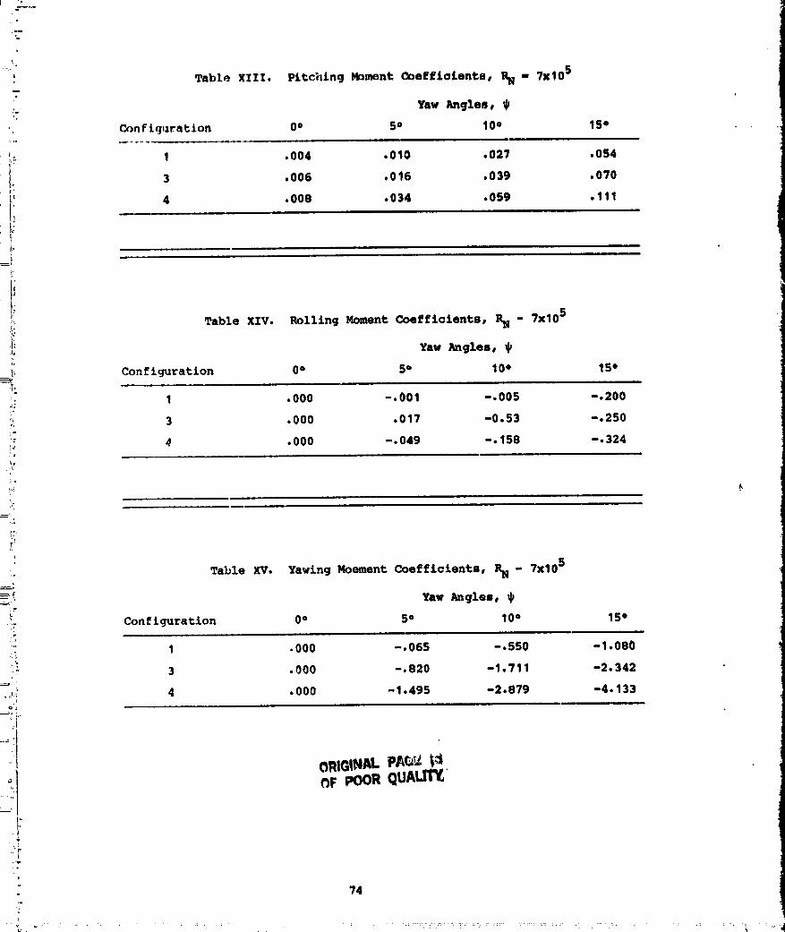
The moment coefficients are contained in Tables XZlle XIV and XV.

The moments were taken about a point on the centerline of the vehicle

106.3 cm (41.9") from the front of the vehicle and 35.6 cm (14.0") above

ground level. The reference area used was the projected frontal area

- (A); the reference length (c} for the pitching moment was the vehicle

0 length; the reference length (c} for the rolling and yawing moments was

the vehicle width. The rolling and yawing moments ware corrected for

"" flow angularity.

4.0 CONCLUSIONS AND RECOMMENDATIONS

The following conclusions can be drawn from the tests conducted.

I. "_ airflow in the subscale model of a representative

. commercial livestock trailer was indeed random and variable. There were

conditions wherein there was virtually stagnant air in some locations

and very rapid air flow (up to 75% of free stream velocity) in other

locations of the cargo compartment. The local internal flow conditions

:," were very dependent on the relative wind angle.

2. The streamlined configuration with a ram air inlet and

- ductlng, vented base and fans can ;)rovide a nearly uniform air flow !i

"'" throughout the trailer under condlti_ns of variable wind angles, wind

: speeds and vehicle speeds (including while the vehicle is not in

::- motion}. This air flow could be adjusted to provide the most d6slrable

::: flow conditions for the cattle. Further, as desired, the Incoming air

: could be heated or cooled and precipitation extracted.

" 3. The streamline configuration with NAC_ submerged inlets and

r vented base could provide better flow conditions than the subscale model I

I..... of the representative commercial trailer. It would be more difficult to

provide the proper air flow at low vehicle speeds, to heat or cool the

14 i

1983018489-TSB11

atr and to remove precipitation with the N&CA nubmer_ed inlets than with

the ram air Inlet conflq_ratlon. Additionally the air aomlng in the

stde ducts would probably be more likely to contain dusts smoke and

other impurities.

4. The streamline vehicles present a significant potential fuel

saving of approximately 98,240 per 160,900 _a (100,000 mi) of operat!on.

It is recommended that a series of full-scale tests be conduated on

a prototype vehicle based upon the configuration 5 design to:

1. btablish the appropriate internal flow rates for different

temperature and loading conditions which are most desirable for various

kinds of animals during tranelt_

2. Establish environmer _al criteria for the design of future

livestock haulers.

3. Define statistically significant livestock and economic losses

experienced with representative conventional haulers as compared t-

prototype haulers having design based primarily on configuration 5.

4. Check the validity of the wind tunnel results.

15

t_

198 3018489-TSB12

5.0 _FE_NCES

I. StOV@nfl, D. G. and Hahi;, G. L., "Air Transport of Livestock -

Environmental Needs," AR_E Papor No. 77-4523, American Society of

Agriculture Englneers Winter _kJotinq, Chicago, Ill., _cember 13-16, 1977.

2, Grandin, q_mplo, "_h_ Bf_ec_ of Stroaa on Livestock and Moat 1Quality Prior to and During Slaughter," INTJ STUD ANZM PROS M(5) i1980.

3. Grandin, Temple, "Handling, Livestock," Agrl Practice, May 1979.

4, Seubert, Terrence V., "Handling & Transport of Bob Calves & SpecialFed Veal Calves," Paper, L.C.I. 66th Annuat _eoting, Louisville,

KF, April 13, 1982.

5, James, Paul E. "Modification of _closed Trailers to Transport

' Disease-_xposed cattle," ABAE Paper No 76-6510 and Structures andEnvironment Division of ASAE Vol 21, No. 3, September, 1977.

: 6. McC_an, H, L. "Double-Decked Stock Truck Cooling and Ventilating

; System," United States Patent NO, 2,612,027, September 30, 1952,

: 7. Saltzman, Edwin J., "Low-Drag Ground Vehicle Particularly Suited

for r_e in Safely Transporting Livestock," United States Patent NO.4,343, 506, AUgUSt 10, 1982.

8. Muirhead, V. U., "An Investigation of Drag Reduction for Tractor

Trailer Vehicles," NASA CR 144877, October 1978.

9. Muirhead, V. U., "An Investigation of Drag Reduction for TractorTrailer Vehicles with Air Deflector and Boattail," NASA CR 163104,

January 1981.

10. Steers, L. L., and Seltzman, E. J., "Reduced Truck Fuel Consumption

: through Aerodynamic Design," Journal of Energy, Vol. I, No. 5,

September-October 1977.

11. Montoya, L. C., Steers, L. L. and SeltEman, E° J., "AerodynamicDrag Reduction Tests on a Full-Scale Tractor-Trailer Combination

and Representation Box-Shaped Ground Vehciles," Society of

Automotive Engineers, SAE Paper 750703, AUgUSt 1975.

12° Montoya, L. C°, and Steers, L° L., "Aerodynamic Drag ReductionTests on a Full-Scale Tractor Trailer Combination with Several Add-

on Devices," NASA TMX-56028, December 1974o

13° Muirhead, V. U., and Saltzman, E° J., "Reduction of Aerodynamic

Drag and Fuel Consumption for Tractor Trailer Vehicles," AIAA paper

79-4153, Journal of Energy, Vol. 3, No° 5, 8eptember-Dotober 1979,

: p, 27g.|

14. Mossman, Emmet A. and Randall, Lauros M., "An Experimental

Investigation of the Design Variables for NACA Submerged DuctEntrances," NACA RM No. A7130, January 1948.

16

6.0 FIGURBB AND TAB_,ES

ORIGINALPAGE13_i _ POORQUAL_Y

I

w

1983018489-TSC02

"_ 20

_i_'! ORIQIIVACPa(_r::r.¢".i:,,. OF POOR QUALITY

_:_: 72 73 74,, ' • • • FrontEnd(F)__:_-. 75 76 77 LookingForward,_i • • •-.,_ 11nslde)

.... .;. i ! ,. ,. ,. q f u

; 78 79 80- • • •

,.i', 81 82 83 BackEnd(B)o_,,. • • •

_,,.; LookingForward:_ 84 8P 80_,: • • • (Inside)

.... 87 88 89

I

..

°,,.:::- Fibre 2.1.4 Ik_essure t:ap locations In baseline trailer model,o- ¢onflguratlon le _ront and rear.

:_:.:; 2] 1i '"

...... ..,\', " .... I- .. '._ ,, : _,o ,,

1983018489-TSC04

ORIGINAEPAGE18POORQUALITY

r_il _-;_'- __ ..... "_

6P,I_IINALrAc;_t_0I: POORQUALITY

:' 24

1983018489-TSC07

'i

i ,.

. _; ORIGINALPAGE IS i. : j ° .OF.POORQUALrI_

: : m

r 2 ............ __ ._- r

l_ C. I " =

.-. I g oz,.

:;\ lii'. . _ o =l OI¢

:: ; j i[.,_l, :- i r _ ,-G Ir_.l /• .__-.--'_ _i° - <__<_Ix/'

t , ,] "tl;: ;:" I /I

' '.: : I -" 14,- ., . !: _I _ "''-

'_ 26 '

1983018489-TSC09

ORIOIN_PAQEISOFPOORQUALITY

I

Figure 2.1.10 Photograph of _orvard streamlining and ram air inlet onoonfiguration S,

27

1983018489-TSC10

" "1

OI_HAI_PA_ IS' OF POORQUALIFY iI

1

28 'J

I ...... _ -; • - "' ;_-_- -.-- -_'' "':;----; _.-.._ " " L _. _. ; _ . ._._ -TT _ -_,_., _..... -._-,.; --,-,-;;,- _ • _.. _ ;t _. :

1983018489-TSCl 1

oF_OORQUA:I'_"

1983018489-TSC13

Olll(llNlll; PAQI[ISOF pOORQUAL|I"f

x _ .._

.mlm X X X

II _ _ "I "' X X x X o

..I -a

_ -_I _1 !_1 / _ X X X X

_ >< x><><l_: ._I----JJl_ I i

IIII II 0 _ x x x x ._

•, ,_?,_ .. x x x x o><_x _i_.,

_. • : :• _ i'M t_ ',i:lr _ _o

: "_Z

31r.

• . , ',,

1983018489-TSC14

7

OiliNg1- pAU M_, loon QOAL.I_

32

1983018489-TSD01

1

i34

1983018489-TSD03

...........................................................................................................................................1983018489-TSD04

36

1983018489-TSD05

38

1983018489-T SDO7

ORIGINAI_PAGEIm i-" _ POORQUALITY.

[

_ h

i

1983018489-TSD08

II

ORIGINALPAGE IllOF.pOOROUAt._

40 i

1983018489-TSD10

1983018489-TSD11

43

1983018489-TSD12

OF POORQtlAl.rr"

44

4b ._

1983018489-TSD14

OmQINA_PAO[ISOFPOORQUAL_Y

46

1983018489-TSE01

47

1983018489-TSE02

5Oi

1983018489-TSE05

51

1983018489-TSE06

q,k

i,;

. " OF.POQ__UALII"Y .m

'I" I

1:1.-_

°' i:, D < 0 &

\,_.Q,.p

T M "# "4. • !

=°,i" IM

.,°4" _

=2.:42 ,4

gI

•o i

" " = _ _" = " = !_ _a " d d d3 - .LN3131..-I_303ov_a

1.

,,I: 52 ' !

.... 19830iS489-TSE07

53

"- ' '.......................:...................................................'-_1983o1 8489-TSE08

ORIGINAL PA_E I$OF POOR QUALITY

55

1983018489-TSE10

i +i;;

*+- OIIIGIN/d_"PAGE18.." O_ POOR QUALITY

_--

,16

tL

:. OD4

7,

,.!

+

,#"

_h

i "¢

: ]i+,+;.

B 8 @ I_ f_ tR q_",:" to:::) J.N30_13d SV 03'_'

"_': 56i ,_

!" l,,+

1983018489-TS E11

ORIGINAL"p,_,__

57

• I. -. +............... . -...... - , i+.L_L,,__. +.+.+.L._++ + i ,_...........-..-+ .... ++........ ++:...... •........... '+.....+..... _,++";"+..... -+?,!::?++ ,.. ",, .:[..." _ ............ +j

1983018489-TB E12

58

......... " ..... i

1983018489-TS E13

..... ,........ m

7t,.

-!F

'i"

_'. OEPOOR(;;lUALrI'X .:

i'

_ J

Li

.,_

'9

:: W

- _

jr

'T

p,' i

: cJ II d d" 3 - .LN3I_I.-I..-130:33:_10.-130IS

°

-, 5g j

1983018489-TS E14

t,")-

_. i +'_--"+_'_+_++-_'" + +++++ .... " ..... ++:'+ "+,0 ,+ ........................ ++- _'+ .... _++'_: .... '+o ++

+ - . ,, _ , ¢.+, .....

198go18489-TSF02

O

;:" :) J.N3:)tJ3dSV "1= I

62

1983018489-TSF03

ORIGINAL PAGE ROF. POOR QUALITY

Table I. Coefflcients of Static Pressuro, ConfiguratLon I

Yaw Angle, _ - 0° RN - 7.52 x 105

' Sides (outside) Top (inside roof)

Left Right Left Center Right

Tap % % Tap cp ep cp

7 -.184 40 -.121 2 -.223 1 -.106 30 -.094

12 -.143 45 -.046 61 -.082 60 -.094 6 -.094

15 -.136 48 -.046 64 -.082 63 -.059 62 -.059

10 -.053 43 -.053Upper De_k

14 -.022 47 +.04667 -.094 66 -.082 65 -.035

8 -.015 41 -.07531 -.070 32 -.070 68 -.082

21 -.106 54 -.11371 -.059 70 -.047 69 -.047

25 -.121 58 -.143

28 -.121 5 +.060 Front (inside)

11 -_075 44 -.03072 -.068 73 -.082 74 -.082

22 -.083 55 -.12175 -.094 76 -.082 77 -.094

26 -.068 59 -.121Rear (inside)

9 -.046 42 -.068

13 -.068 46 -.068 78 -.117 79 -.106 80 -.129

20 +.030 53 -.083 81 -.106 82 -.117 83 -.129

27 +.046 4 -.030 84 -.106 85 -.106 86 -.106

16 -.121 49 -.128 87 -.117 88 -.106 89 -.117

18 -.121 51 -.136Lower Deck

23 -.121 56 -.14339 -.068 36 -.068 33 +.030

, 17 -.121 50 -.14338 -.075 35 -.075 3 -.060

19 -.098 52 -.11337 -.075 34 -.083 29 -.070

24 -.113 57 -.128

63

1983018489-TSF04

o ,,

F'--

' ORIGINALPAGE I_i OF POORQUALITYi-b.

i'

I' Table Z. Ooeffielents of Static Pressure, Confi_ratlon I

Sides (outside) Top (inside roof)

' i Left Rifht Left Center Right

r

,.,o

, 7 -.311 40 -.193 2 -.206 1 -.182 30 -.194

;_: 12 -.359 45 -.065 61 -.147 60 -.182 6 -.324

_. 15 -.355 48 -.041 64 -.135 63 -.124 62 -.194

J ._ 10 -.189 43 +.026,_ Upper Deck

_ 14 -.174 47 +.102_ 67 -.182 66 -.182 65 -.100

_'_' 8 -.144 41 -.087: _ 31 -.135 32 -.147 68 -.171_ ' 21 -.242 54 -.140

,o, 71 -.124 70 -.118 69 -.112

i _ 25 -.258 58 -.200!:. 28 -.272 5 .000 Front (inside)

i ? 11 -.174 44 -.019 72 -.174 73 -.171 74 -.159

_ - 22 -.174 55 -.200 Ii il 75 -.182 76 -.171 77 -.171!_,: 26 -.174 59 -,079i:, _ Rear (inside)_o_" 9 -.174 42 -.072

._ 13 -.181 46 -0065 78 -.194 79 -.194 80 -.218

- 20 -.038 53 -.041 81 -.182 82 -.206 83 -.194

_. 27 -.038 4 -.046 84 -.194 85 -.194 86 -.171

_' 16 -.234 49 -.200 87 -.182 88 -.182 89 -.171

" 18 -.234 51 -.193_: Lower Deck

23 -.242 56 -.185' :" 39 -.140 36 -.132 33 -.012_.,!_... 17 -.242 50 -.215

_/_ 19 - 196 52 - 193 38 -.140 35 -.140 3 -.144.._ 37 -.140 34 -.140 29 -.152:: 24 -.234 57 -.193

D

! '

! 64

1983018489-TSF05

o ORIGINALPAGEIS ,

O[ POORQUALIFY !

Table _. Coefficients of Static l_essure, Configuration 1

Yaw Angles _ = 10° RH = 7.42 x 105

Sides (outside) Top (inside roof)

, Left Right Left Center P_L_lt i

4

7 -.454 40 -.198 2 -.291 1 -.338 30 -.314

12 -.462 45 -.023 61 -.279 60 -.303 6 -.457

15 -.454 48 -.023 64 -.208 63 -.184 62 -.267

10 -.293 43 +.114Upper Deck

14 -.248 47 +.24567 -.291 66 -.327 65 -.184

8 -.248 41 -.06131 -.208 32 -.270 68 -.243

21 -.324 54 -.16071 -.160 70 -.160 69 -.220

25 -.317 58 -.176

28 -.332 5 +.004 Front (inside)

11 -.255 44 +.02372 -.293 73 -.315 74 -.267

22 -.233 55 -.22175 -.290 76 -.290 77 -.279

26 -.261 59 -.053_ar (inside)

9 -.271 42 -.084

13 -.293 46 -.061 78 -.255 79 -.243 80 -.290

20 -.110 53 .000 81 -.232 82 -.290 83 -.196

27 -.088 4 -.026 84 -.243 85 -.243 86 -.220

16 -.317 49 -.260 87 -.232 88 -.232 89 -.230

18 -.317 51 -.252Lower Deck

23 -.324 56 -.21439 -.183 36 -.176 33 -.031

17 -.340 50 -.29038 -.214 35 -.191 3 -.195

19 -.29_ 52 -.26037 -.221 34 -.207 29 -.195

, 24 -.333 57 -.267

i

85

" ..............."....' " 1983()18489-TSF06

_ :,,

t

ORIGINALPAGE18.., e t

OF POORQUALITY

" Table I. CoeffLc£ents o_ RatLc Pressure, CDn£Lgurat£on 1

Yaw Angle, ¢ - 15° 1_ = 7.42 x 105

•v Sides {outs£de) Top (/neLde roof)e

,.. Left l_Lght I4ft Center Right

Tap ep Tap ep % ep Tap %: 7 -.481 40 -.076 2 -.362 1 -.386 30 -.374

: 12 -.474 45 +.061 61 -.327 60 -.421 6 -.564

": 15 -.474 48 +.069 64 -.148 63 -.220 62 -.338

: 10 -.314 43 +.153,_.. Upper Deck2-,.. 14 -.352 47 +.450{ 67 -.362 66 -.410 65 -.255,:_ 8 -.314 41 +.061:r

31 -.243 32 -.267 68 -.291_ 21 -.397 54 -.122

:_ 25 -.381 58 -.100 71 -.184 70 -.184 69 -.196

_ 28 -.352 5 -.007 Fz'ont (inside)

: 11 -.352 44 +.061_; 72 -.357 73 -.386 74 -.338,'" 22 -.328 55 -.191.'t 75 -.362 76 -.374 77 -.350c 26 -.357 59 -.015

Rea_ (ine£de)-_"i 9 -.381 42 -.061

,._ 13 -.397 46 -.038 78 -.303 79 -.291 80 -.350

: 20 -.254 53 +.046 81 -.255 82 -.327 83 -.220

27 -.167 4 .000 84 -.291 85 -.279 86 -.232

r 16 -.405 49 -.267 87 -.291 88 -.267 89 -.22018 -.412 51 -.207

,"_ Lower Deck.:, 23 -.428 56 -.167, 39 -.307 36 -.221 33 -.069

17 -.435 50 -.390

= 19 -.405 52 -.359 38 -.267 35 -.274 3 -.252ii" 37 -.283 34 -.274 29 -.252>-; 24 -.443 57 -.359

e

<.

- 66

1983018489-TSF07

Table II. Internal Air Flow Speeds, Conf£guration 2

Location Yaw Angle, _- 0 •

Right Middle Left

A 7.9 (25.8) -4.4 (-14.4) Small (Small)B -3.4 (-11.3) 2.8 ( 9.2) 4.B (15.9)C 7.1 (23.4) 5.2 (17.2) 6.3 (20.6)

' D -3.4 (-11.2) -2.0 t -6.5) -2.0 (-6.5)E S_11 (Small) 3.4 (11.3) 2.8 ( 9.2)P 6.2 (20.6) Small (Small) -2.8 (-9.2)

Location Yaw Angle, _ =, 5"

Right Middle L_ft

A 14.5 (47.5) 5.9 (19.5) 2.0 (6.5)B 3.4 (11.3) 2.8 (9.2) 2.0 (6.5)C 16.6 (54.4) 12.4 (40.6) 4.8 (15.9)D -2.0 (-6.5) 3.4 (11.3) 4.5 (14.9)g -2.0 (-6.5) 5.9 (19.5) Small (Small)P 2.0 ( 6.5) _._tall (St.all) -4.8 (-15.9)

Location Yaw Angle, $ = 10"

Right Middle Le ft

A 24.9 (81.7) 15.1 (49.5) 8.2 (26.8) kB 3.4 (11.3) Small (Small) -2.0 (-6.5)C 22.1 (72.7) 17.7 (58.2) 2.0 ( 6.5)D 4.8 (15.9) 7.4 (24.3) 2.8 ( 9.2)E 4.4 (14.5) 7.4 (24.3) -2.0 (-6.5)P 4.4 (14.5) -3.4 (-11.3) -6.6 (-21.6)

Locatlon Yaw _Igle, $ = 15•

Right _iddle Left

A 24.0 (78.8) 17.9 (58.9) 9.1 (29.8)

B 13.6 (44.6) 8.9 (29.1) -2.0 (-6.5)C 13.4 (44.1) 22.3 (73.3) 2.0 ( 6.5)D 5.9 (19.5) 9.6 (31.6) 2.0 ( 6.5)E 3.4 (11.3) 7.1 (23.4) 4.0 (13.0)

• F 6.2 (26.8) -7.9 (-26.0) -8.4 (-27.6)

K_r flow speeds in meters/see (ft/sec) with flow from front to rearpositive

Small tnd£catee air flow speed of less than .9 m/see (3 ft/seo), ipositive or negative.

Wind tunnel aLrspeed 33.5 m/see (110 ft/seo)

67

1983018489-TSF08

•_' CRIGINALPAGE13

OF POORQUALITY

-: Table lit. Internal _ir _low _eeas, Configuration 5

Lr--

: T_e_tLon Yaw Angle, _ = 0 •

.i: Ri ght Middle Left

-_ A 4.4 (14.5) 5.9 (19.4) 4.4 (14.5)

.: B 2.0 (6.5) 5.6 (18.3) 4.0 (13.0) _:, C 5.2 (17.1) 3.4 (11.2) 2.8 ( 9.2) ,

i_ D 3.4 '11.2) 2.8 (9.2) 2.0 (6.5):r E 4.0 (13.0) 3.4 (11.2) 4.0 (13.0)

v 4.0 (13.0) 2.8 (9.2) 2.s (9.2)

•= Location Yaw _gle, $ = 5°

Right Middle Left

2.8 ( 9.2) 4.8 (15.9) 4.0 (13.0)" B 2.0 (5.5) 5.2 (17.1) 3.4 (11.2):_ C 4.4 (14.5) 2.0 (6.5) 4.4 (14.5)

D 4.0 (t3.0) 4.0 (13.0) 2.8 (9.2)_ E 3.4 (11.2) 4.4 (14.5) 3.4 (11.2)

F 4.0 (13.0) 4.0 (13.0) 2.8 ( 9.2)i:

/ Location Yaw Angle, _ = 10°

Right Middle Left

_ A 4.0 (13.0) 4.8 (15.9) 4.8 (15.9)B 2.0 (6.5) 6.2 (20.5) 4.8 (15.9)C 4.0 (13.0) 4.0 (13.0) 5.2 (17.1)D 2.0 (6.5) 2.8 (9.2) 3.4 (11.2)

" E 2.8 (9.2) 4.0 (13.0) 2.0 (6.5), _ 3.4 (11.2) 3.4 (11.2) 3.4 (11.2)

Location Yaw Angle, $ = 15 °

": Right Middle Left

T A 2.8 (9.2) 4.0 (13.0) 4.4 (14.5)B 3.4 (11.2) 6.2 (20.5) 4.4 (14.5)

_ C 3.9 (12.9) 4.0 (13.0) 3.4 (11.2)O 4.4 (14.5) 3.4 (11.2) 2.0 (6.5)E 4.4 (14.5) 3.4 (11.2) 2.8 (9.2)

-_ F 4.S (15.9) 4.4 (14.5) 2.8 (9.2)

ALr _low spoed_ in meters/see (ft/see) with flow from front to rear= positive

Smalt tndLcates aLr flow speed of less than .9 m/see (3 ft/eee),

poeLtLve or negative.

'; Wind tunnel airspeed 33.5 /seu (110 ft/eee)

68

L ' i "

1983018489-TSF09

i"

- ORIGINAL PAGE 18:': D_. POOR QUALITY

.'._ Tahl_ _V, Internal _[r _lc_ _eods, CJ_nfiqurakLrm 6

- Loo_ion Yaw Angle, ¢- O.#

Right Middle Left:

" A 2.8 ( 9.1) 2.8 ( 9.1) 2.8 ( 9.1),',',::', FJ Small (Small) Small (Small) Small (Small)" C 2.0 ( 6.5) 2.0 ( 6.5) 2.8 ( 9.1): D 2.0 ( 6.5) 2.0 ( 6.5) 3.4 ( 11.2)

g 2.0 ( 6.5) 2.8 ( 9.1) Igumll (S_aall)i :_ I;' 2.0 ( 6.5) 2.0 ( 6.5) 2.0 ( 6.5)

i i_ Looation Yaw Angle, ¢ - 5"

....... Right Middle Left

_, A 2.0 ( 6.5) 2.0 ( 6.5) Small (Small)

_ _ B 2.0 ( 6.5) 2.8 ( 9. t) Small (Small)_ C Small (Small) 2.8 (9.1) Small (Small)

./ D Small (Small) 2.8 ( 9.1) 2.0 ( 6.5)g Small (Small) 3.4 (11.2) 2.0 ( 6.5)F Small (Small) 2.0 ( 6.5) 3.4 ( 11.2)

r,

, Location Yaw Angle, _ = 18 °

°:i" Right Middle Left

:: A 2.8 (9.1) 2.0 ( 6.5) Small (Small):- B 3.4 (11.2) 2.0 ( 6.5) Small (Small)

c Sma]1 (small) 2.0 ( 6.5) -2.0 (-6.5),. D 2.0 (6.5) 4.0 (13.0) -2.8 (-9.1)..i: E Small (Small) 3.4 (11.2) 2.0 ( 6.5)

_" 2.8 (9.1) 2.8 (9.1) 2.0 (6.5)

: Location Yaw Angle, _ = 15•

._,- Right Middle Left

.." & 2.0 ( 6.5) 2.0 ( 6.5) 13mall (S_all)_:: B 2.8 ( 9.1) 2.0 ( 6.5) 2.0 ( 6.5)?" C 2.0 ( 6.5) 2.0 ( 6.5) 2.0 ( 6.5)i

._: , P 2.8 ( 9.1) 3.4 (11.2) -2.0 (-6.5)_.. E 2.0 ( 6.5) 3.4 (11.2) 2.0 ( 6.5).'._" F 2.0 ( 6.5) 3.4 (11.2) -2.0 (-6.5)

.'. &It air flow speeds in meters/see (ft/seo) with flow from front to rear" pos itire

i!_ Small. indicates air flow speed of less than .9 m/seo 13 ft/sec),'_.': p_sitive or negative 1

6..;- Wind tunnel alrspeed 33.5 m/seo (110 ft/seo)

!-/ 69

I,

= r,

1983018489-TS F10

J

Table V. Internal _ir Flow Volumes for Nodelse

Configuration Yaw _mgles,

• Number O• 5 • 10 • 15 •

-; 2 upper .018 (.62) .104 (3.69) .169 (5.97) .243 (8.60)

2 lower .110 (3.90) .169 (5.96 .240 (8.51) .234 (8.27).m

, Total .128 (4.521 .273 (9.651 .409 (14.48) .477 116.871

5 upper .089 (3.16) .075 (2.66) .091 ( 3.21) .086 ( 3.04)y

, 5 lower .076 (2.69) .091 (3.21) .081 (2.87) .089 (3.16)

; Total .165 (5.85) .166 15.871 .172 ( 6.081 .175 ( 6.20)

6 upper .028 (1.00) .030 11.05) .035 (1.22) .036 (1.28)

6 lower .060 12.11) .032 (1.13) .013 ( .47) .043 (1.52)

:" Total .088 (3.11) .062 12.181 .048 (1.69) .079 (2.80)

Volume, m3/se_ (ft3/s)

Wind tunnel airspeed, 33.5 m/se_ 1110 ft/se_)

Y

T

q

70

1983018489-TS F1;I

i *ii*

'' ORIGINAL PAGE ISOF POOR QUALITY

, " Table VI. Meltlnq Times eor Ice Cubes erom Internal _Lr Flow, ,Con_Iguratlon 2

Yaw ,_,nglee,Location O" 50 10° 15°

Test Section 2.2 2.2 2.2 2.2._ 2.4 5.6 5.6 5.4B 8.5 4.9 6.2 3.4

C 6.5 4.3 4.2 4.1 \D 8.0 4.6 5.3 5.5E 14.3 8.6 8.3 8.5P 12.6 10.2 7.4 7.3

,] ' G 4.8 4.5 5.5 4.4H 5.4 5.2 5.0 6.6

I 1.6 2.5 2.7 7.0J 1.6 2.2 2.3 3.8K 9.7 6.2 8.7 7.1

_*_ I, 1• 9 1• 9 2.1 2.5

_;, &ll times in minutes and corrected to a tunnel test section temperature

i Of 26.70C (80°C)

_;! Wind tunnel airspeed 33.5 m/sec (110 ft/sec)

j,

_

: Table VII. Melting Times for Ice Cubes from Internal Air Flow,

_ Configuration 5

,i Yaw Angles, $

" _' Location 0° 5° 10° 15°

_, Test Section 2.2 2.2 2.2 2.2

:_ A 5.4 6.1 5.8 5.8. 6.6 8.6 lO.3 12.oc 7.6 9.9 11.5 lO.3D 8.8 9.8 8.5 8.6

J_

!i _ 5.8 7.3 7.4 9.5_ F 7.9 7.e 6.9 8.1G 4.2 3.4 5.0 7.7

_! H 9.8 11.9 14.1 11.7i . I 11.5 9.1 10.5 14.8

! J 10.4 9.5 12.1 14.8_I K 14.4 11.7 19.0 17.0_ 1, 4.1 4.3 3.8 3.9

_ t_ All times in minutes and corrected to a tunnel test section temperature

of 26.7oC (80oF)

Wind tunnel airspeed 33.5 m/sec (110 ft/sec)

1983018489-TSF12

P

Table VIII. Halting Times for Ice Cubes from Internal Flow,

Configuration 6

Yaw Angles,Louatlon 0e 5" 10" 15 e

Test Section 2.2 2.2 2.2 2.2& 6.3 6.9 6.9 7.4B 11.7 12.3 11.4 7.4C 14.0 16.4 15.7 18.9D 14.7 13.3 17.5 17.4

: E 16.9 15.0 17.9 17.0P 15.4 13.4 15.2 17.7G 9.8 13.4 16.0 14.8H 18.6 18.6 22.1 24.0I 9.5 13.9 12.9 13.6

J 14.8 17.6 14.2 15.2K 26 •5 26.3 26 •0 29.0L 25.4 21.7 25.:) 17.00'

All times in minutes and corrected to a tunnel temperature of

26.7"C (80"P)

Wind tunnel air speed 33.5 m/seo (110 ft/sec)

Table IX. Drag Coefficients

Yaw angles,

Configuration 0" 5" 10. 15" Average Reynolds No.

1 1.070 1.570 2.080 2.640 1.840 7x105

3 .816 1.195 1.743 2.448 1.550 7x105

4 .579 .?78 1.239 1.838 1.109 7x105

No. 1

(NASA CR 144877) .990 _.110 1.362 1.519" 1.245 6X105

• HO. 4!_ (NASA CR 144877) .592 .750 .960 1.082" .846 6x105

No. 5

" (NASA CR 144877} .506 .560 .646 .688* .600 6xi05

*Average of 10" and 20° data.

72

198;3018489-TS F1;3

m

'PabL,_ g. PotentL,_.t I_el and Rconomtc Savtngn of Modi.fLnd- VahtaZ_n R_l_t,tve to Configpzra_ton_ 1 and 21

Fual Ej,,neL_y ,avin_m p_.ml o_st _vin_s

• C,)nft,i,lr,lg[nn liLer_ (gal/hr 21 LItarl (qal) 3 $/hr 4 $ 3,4

" ] 7.7 12.01 14,063 13,740) 3.04 3e715

_. 4, 5, 6 17.2 (4.5) 31,190 (8,240) 4.53 8,240

1 Vohir.le speed 88.5 Km/hr (55 nph), annual national average winds 15.3"_ Km/hr 19.5 mph)

.. 2 Brake specLfL¢ fuel consumption - 2.129xlO'4kg of fuel per watt-hour: (0,35 pounds per horsepower-hour) Diesel fuel density 0.834 kg/liter

; 16.96 Zb/gal).

- 3 _ssumed mLleage - 160,900 Km per year (100.000 ml per year).

4 _ssumed fuel cost = 26.4 cents per liter (1 dollar per gal.)

'" Table Xl. Side Force Coefficients, RN - 7x10 5

Yaw angles,

Configuration 0° 5" 10° 15°

1 .000 .235 .396 .438

3 .000 .511 .922 1.271

4 .000 .632 1.195 1.562

No. 1(HASA CR 144877 .000 .520 1.220 2.040*

*Average o_ 10° and 20" dataY

,.q

Table XZI. Lift Coef_icLents, P.._ 7 x 105pl

'; Yaw Angles,

Con fL_juration 0 ° 5° 10° 15 °

1 .087 .258 .490 .790

-__ 3 . 108 • 442 .736 1. 003

-- 4 .162 .316 .612 .975

:

:;

'_ 73

,.... " _ - ;_ : _ _ - '_ =- "; ..... ":: _= -" - - _ -- _: -- " ....._ --_-.,. "" "i ".:-_,:,; '::.:.:.:......-..-.,_............. .....•..........,41...... _;. .-:"" _ :-_ ._:?_:_: _ U= ".... _ -;?- :- :_" - -_:_- _ ?-

L.J

1983018489-TS Fi4

--,

Table XIII. Pitching Moment Coeffiolentss _- 7x10 §m r

Yaw ;ingles e

ConFiguration 0° 5° lOe 1Se

t_ 1 .004 .010 .027 .054

I 3 .006 .016 .039 .070I: 4 .008 .034 .0S9 .111

tt, t

=!!"

.i! Table XIV. Palling Moment Coeffioients, RN - ?xl0 S!:

[i Yaw Angles, 0

;i Configuration 0° 5° 10" 15 °

;;_ 1 .000 -.001 -.005 -.200J

3 .000 .017 -0.53 -.250

:: 0 .000 -.049 -.158 -.324

_w

).r

'F

.' Table XV. Yawing Moement Coeffiaients, RN - 7x105

_ Yaw Angles,

ConEiguration 0° 5° 10" 15°

' 1 .000 -.065 -.550 -1.080

: 3 .000 -.820 -1.711 -2.342

....,_ 4 .000 -1.495 -2.879 -4.133

)1 oF QUAm"L..F

r

" 74

1983018489-TSG01

7.0 &PPENDIX

pOWERR_UI_D

The model data for Configuration 1 were applied to the full aise

prototype vehicle at a road speed of 88.5 km/hr (SS mph). The wind

component was rotated from 0 ° _.o 180 e. The wind speed used was 15.3 km/hr

(9.S ._h).

t

ORIGtHAtPAGEISOFpOORquALrrY

V2_ -

V = Relative wind speed

V I = Ground speed

W = Actual wind velocity

V2 = Side wind velocity component

B = Wind angle relative to the vehicle path

= Relative wind angle

,5 i4

L

Q_.. --_ O"_ j' _' ,,J L. , .....,

1983018489-TSG02

7.1 Power to Overcome _rodynamic Drag - Confi_uration 1

The power required is s

D V1 ORIWNAI.Pjllmt III* P = 100"--_kw (Multiply by 1.341., hp) OF POOR (_U_'r_

where• i

":_ D = I/2OV2CDA

A = 9.15 m2 (98_6 ft 2) - Full s_ale vehi_le

p : 1.226 kg/m 3 (.002378 eluge/ft 31

:' CO is taken from Figure 3.4.2 for Configuration 1 at approximate

values of _.

Example:

" V I : 88.5 km/hr or 24.58 m/see (55 mph)

W = 15.3 km/hr or 4.25 m/see (9.5 mph)

8 : 15°

Relative wind angle:

-I W sinB:" _ = Tan

V 1 + W oosB

-I 15.3 km/hr sin 150

- Tan 88.5 km/hr + 15.3 kz/hr oos 15g

: 2.19 o

• From Figure 3.4.2:

-. CD1 = 1.28- Then •

,.:" D = 1/2x 1.226 x (28.71) 2 (1m

28) (9.15)

.;- D = 5917.8 N i

:. p = (5917.8) (24.58) = 145.5 kw (195.1 hp) t:. 1000

76

1983018489-TSG03