© 2016 wanlin du all rights reserved
TRANSCRIPT

© 2016
Wanlin du
ALL RIGHTS RESERVED

THE INFLUENCE OF PROCESSING PARAMETERS ON
PIEZOELECTRIC AND DIELECTRIC PROPERTIES OF DOME-
SHAPED PZT-EPOXY ACTUATORS
BY WANLIN DU
A thesis submitted to the
Graduate School-New Brunswick
Rutgers, The State University of New Jersey
in partial fulfillment of the requirements
for the degree of
Master of Science
Graduate Program in Mechanical & Aerospace Engineering
Written under the direction of
Kimberly Cook-Chennault
and approved by
---------------------------------------
---------------------------------------
---------------------------------------
New Brunswick, New Jersey
May, 2016

ii
ABSTRACT OF THE THESIS
The influence of processing parameters on piezoelectric and dielectric
properties of dome-shaped PZT-epoxy actuators
by
WANLIN DU
Thesis Director:
Professor Kimberly Cook-Chennault
Thick film dome-shaped two-phase (lead zirconate titanate (Pb [ZrxTi1-x] O3(0≤x≤1))-
Epoxy) structures have been fabricated using a modified sol-gel and spin-coat deposition
process. Processing parameters and poling technique (Corona versus contact poling)
were studied to elucidate their influences on piezoelectric and dielectric properties. 3
primary studies were carried out in the investigation. To study how time/speed profiles in
spin-coating process influence the dielectric and piezoelectric properties of the samples, 4
different time/speed profiles built up form original profile were tested. Poling conditions,
such as corona poling and contact poling were studied at the same material structure and
compositions. Different poling voltages (45kv/mm and 70kv/mm) with corona poling
techniques at low volume fractions of PZT (i.e. 0.1~0.3) were studied on samples fabri-
cated with same techniques to investigate the influences of poling voltage. The combina-
tions of depositing technique and viscosity were studied at low volume fractions such as
0.35 volume fraction of PZT to address the uniformity issue in thickness at lower volume
fractions. The piezoelectric strain coefficient d33 for this dome structure was 9 times
iii
higher than that previously reported values for a composite PZT-epoxy dome structure of
similar structure and composition. The sample morphology was examined with the aid of
scanning electron microscopy (SEM) images and the material distribution was studied by
energy dispersive x-ray spectroscopy (EDS). The piezoelectric strain coefficients, capaci-
tance and effective dielectric constant increased with increasing PZT content. Samples of
all volume fractions of PZT (i.e. 0.1~0.7) that were Corona poled allowed for higher pol-
ing voltages (45 kV/mm compared to 2.5kv/mm in contact poling), and exhibited higher
values of piezoelectric strain coefficients with same material composition , longitudinal
piezoelectric coefficient (@110Hz), effective dielectric constant (@2kHz), and dielectric
loss (@2kHz), were 11.1 pC/N, 28.7 and 0.004 respectively for the PZT volume fraction
equal to 0.7.. The piezoelectric properties were examined both in terms of piezoelectric
effect and converse piezoelectric effect. Piezoelectric strain coefficients and capacitance
were measured @110Hz by Piezometer, and displacement of certain volume fractions of
PZT were studied by Keyence interferometer. To better examine the polarization-electric
field relation, P-E hysteresis loop were measured. Other dielectric properties such as con-
ductance, resistance, and impedance spectrum verse increasing frequency were obtained
by Hp impedance analyzer within the frequency range from 2kHz to 20Mhz. Investiga-
tion of composite structures such as these may lead to development of actuators with en-
hanced displacement and sensors with better sensitivity.

iv
Acknowledgement
First of all I want to show my appreciation to my advisor Prof. Kimberly Cook-
Chennault, she has been continuously supportive for my research and my personal im-
provement as well since the first day I joined the research family. She provides invalua-
ble insights and inspiriting point of view when I experienced research difficulties. With-
out her guidance and persistent help, this thesis would not have been possible.
Besides my advisor I would like to thank my committee members, Prof. Alberto Cuitino
and Prof. Shahab Zadeh for their encouragement, time and helpful insight towards my
research work.
I would like to thank the formal and present members of HESML, Sankha Banerjee,
Udhay Sundar, Andrew Tang, Rui Wang, Eric Bickford and under graduate James Palm-
er, Niasia Williams, Jordan Hoyt (summer intern) for their support and help. Especially, I
want to thank Sankha Barnerjee, as he has been my mentor not only in the research but
also my graduate students life and career. Also I want to thank Udhay Sundar, for being
so helpful and supportive during these years in research.
Lastly, I want to thank my parents as they have been incredibly patient and supportive,
they have always put my happiness on their minds. I would like to thank and show great
appreciation to my husband Wenjie, who has been with me for up and downs, good and
bad times. He has been so caring and patient, and motivated me gently in my research.
Wanlin du
Rutgers University
May 2016

v
Table of Contents Abstract of the thesis ........................................................................................................ ii
Acknowledgement ............................................................................................................ iv
List of Figures ................................................................................................................. viii
List of Tables ................................................................................................................... xii
1. Introduction ................................................................................................................... 1
1.1 Background .......................................................................................................... 1
1.2 Research Goals and Hypotheses .......................................................................... 3
1.3 Research Materials and Methodology .................................................................. 4
1.4 Overview of the organization of the thesis........................................................... 5
2. Definitions, Fundamental Concepts and Literature Review..................................... 6
2.1 Dielectric Materials .............................................................................................. 6
2.2 Polarization........................................................................................................... 8
2.3 Piezoelectric material ......................................................................................... 13
2.4 Ferroelectrics ...................................................................................................... 19
2.5 Polarization Techniques ..................................................................................... 24
2.5.1 Parallel Plate Contact Poling ...................................................................... 24
2.5.2 Corona Poling ............................................................................................. 25
2.6 Composite Materials .......................................................................................... 26
2.7 Spin-coating process .......................................................................................... 31
2.8 Literature review ................................................................................................ 32
2.8.1 Composite piezoelectric materials .............................................................. 32
2.8.2 Curved/Dome shaped piezoelectric devices ............................................... 36

vi
3. Methodology ................................................................................................................ 43
3.1 Chapter Organization ......................................................................................... 43
3.2 Materials ............................................................................................................. 44
3.3 Original and Modified Methodology ................................................................. 44
3.4 Piezoelectric and Dielectric Characterization .................................................... 48
3.5 Characterization of Surface Morphology and Particle Distribution................... 50
3.6 Spin-Speed/Time Profile Study .......................................................................... 50
3.7 Deposition technique Study ............................................................................... 51
3.8 Device displacement .......................................................................................... 56
3.9 P-E hysteresis ..................................................................................................... 57
4. Results and Discussion ................................................................................................ 58
4.1 Chapter Organization ......................................................................................... 58
4.2 Epoxy Dome Device .......................................................................................... 58
4.3 PZT-Epoxy Dome Results for Optimized Fabrication Method ......................... 61
4.4 Spin-speed/time profile study............................................................................. 77
4.5 Deposion technique study .................................................................................. 78
4.6 Summary of the Optimized Processing Conditions ........................................... 81
4.7 Displacement measurement................................................................................ 82
4.8 P-E Hysteresis loop. ........................................................................................... 83
5. Conclusions and Future work .................................................................................... 85
5.1 Conclusions ........................................................................................................ 85
5.2 Future work ........................................................................................................ 87

vii
References ........................................................................................................................ 88

viii
List of Figures
Figure 2.1: (A) Normal state of dielectric material, the dipoles are randomly oriented.
(B) Under the influence of external electric field, the dipoles are aligned. ........................ 6
Figure 2.2: (A) Example for non-polar dielectrics, no permanent dipole moments
possessed. (B) Example for polar dielectrics, permanent dipole moments are randomly
oriented. .............................................................................................................................. 7
Figure 2.3: Schematic of a dipole pair that is comprised of a positive and negative
charged centers.................................................................................................................... 8
Figure 2.4: Mechanisms of electronic polarization. In (A) there is no external electric
field applied. Thus, there is no permanent dipole moment. In (B) an external electric field
is applied, and dipole moments are induced, which results in the alignment of the dipoles
within the material. ............................................................................................................. 9
Figure 2.5: Mechanism of ionic polarization: (A) Without the presence of the external
electric field, positive and negative’s gravity center are coincident, there is no permanent
dipole moments. (B) With the externally applied electric field, gravity centers of positive
and negative charges are separated; dipole moments are induced and aligned. ............... 10
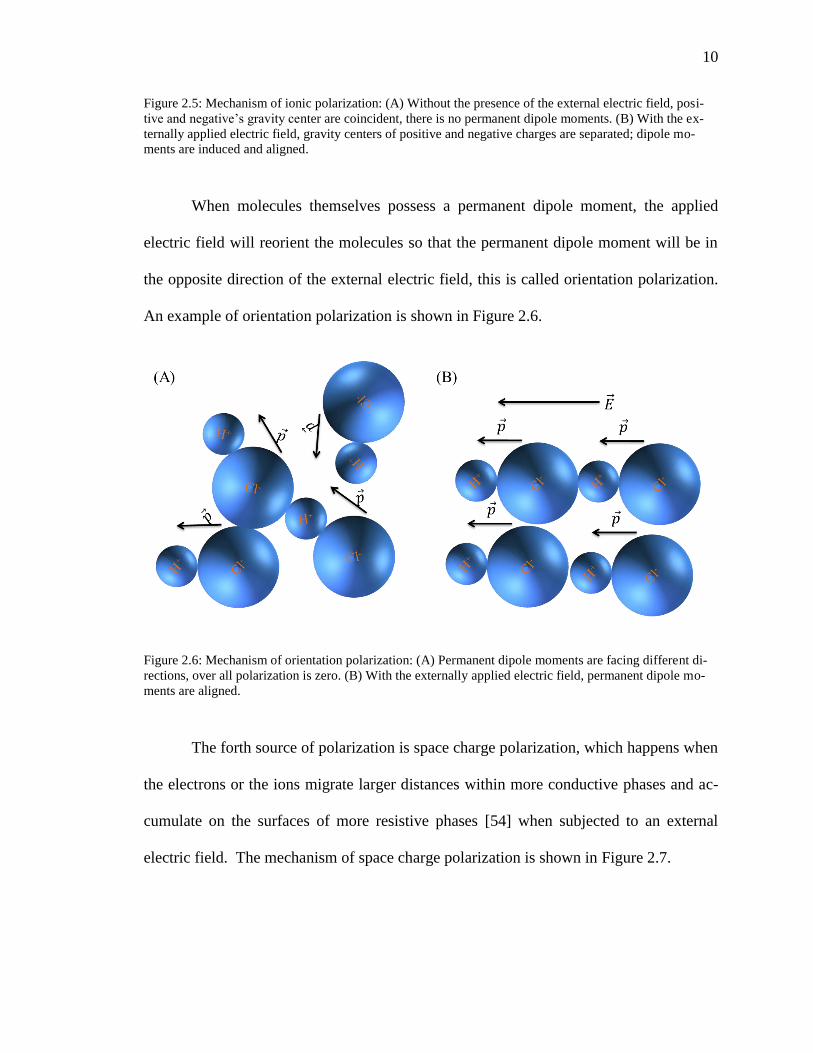
Figure 2.6: Mechanism of orientation polarization: (A) Permanent dipole moments are
facing different directions, over all polarization is zero. (B) With the externally applied
electric field, permanent dipole moments are aligned. ..................................................... 10
Figure 2.7: Mechanism of space charge polarization: (A) Without external electric field,
the ions are mixed up. (B) At the presence of external electric field, the ions could travel
larger distance inside the material..................................................................................... 11
Figure 2.8: Real part and imaginary part of relative complex permittivity ...................... 12
Figure 2.9: Polarization induced by mechanical stress. (A) Without applying the
mechanical stress, positive and negative charge centers are in coincidence. (B) After the
mechanical stress is applied, the dipole moment is induced. ............................................ 14
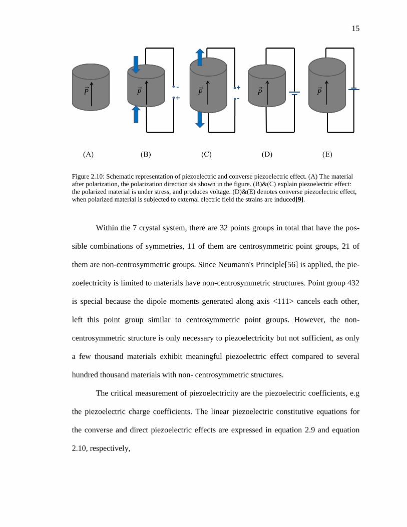
Figure 2.10: Schematic representation of piezoelectric and converse piezoelectric effect.
(A) The material after polarization, the polarization direction sis shown in the figure.
(B)&(C) explain piezoelectric effect: the polarized material is under stress, and produces
voltage. (D)&(E) denotes converse piezoelectric effect, when polarized material is
subjected to external electric field the strains are induced[9]. .......................................... 15
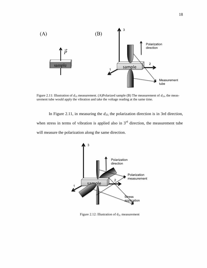
Figure 2.11: Illustration of d33 measurement. (A)Polarized sample (B) The measurement
of d33, the measurement tube would apply the vibration and take the voltage reading at
the same time. ................................................................................................................... 18
Figure 2.12: Illustration of d31 measurement .................................................................... 18

ix
Figure 2.13: P-E relation of normal dielectrics ................................................................. 20
Figure: 2.14 Hysteresis loop pf ferroelectrics[46] ............................................................ 20
Figure 2.15: Hysteresis loop of ferroelectrics with original polarizing path[57] ............. 22
Figure 2.16: Tetragonal perovskite structure below Curie temperature[9] ....................... 23
Figure 2.17: Cubic perovskite structures above Curie temperature[9] ............................. 23
Figure 2.18: Sketch of conventional contact poling set-up ............................................... 25
Figure 2.19: Sketch of corona poling set-up ..................................................................... 26
Figure 2.20: Here shows 10 connectivity pattern families, especially in {0-1}, {0-2}, {0-
3}, {1-2},{1-3} and {2-3} families, each of them include 2 connectivity patterns, which
makes total number of connectivity pattern16[60]. .......................................................... 28
Figure 2.21: Schematics of typical piezoelectric ceramic composite structures [23] ....... 29
Figure 2.22: Scheme of spin coating technique ................................................................ 32
Figure 3.1: Overview of the original method used from our previous work. Appropriate
amounts of PZT, DEGBA and ethanol were measured and mixed with the aid of a
sonicator for 1 hour in the presence of air. The DEGBA binder was then added and the
subsequent mixture was sonicated for an additional 30 minutes. The final mixture was
spin-coated onto dome shaped substrate and cured at 75C. Samples were subsequently
Parallel-Plate Contact poled at~2.2kV/mm [31]. .............................................................. 46
Figure 3.2: Overview of the method of fabrication used for this work. The appropriate
amounts of PZT, DEGBA and ethanol were weighed and then mixed via a sonicator for 2
hours in the presence of air. The mixture was subsequently dessicated for 4 hours to
eliminate air bubbles. The mixture was sonicated for an additional hour. The binder was
then added to the mixture and sonicated again, for an additional 30 mins. The final
mixture is spined coated onto dome-shaped stainless steel substrate, and cured at 75C.
Samples were poled via corona discharge. ....................................................................... 47
Figure 3.3: The dimensions for the dome shape mold. ..................................................... 47
Figure 3.4: The thickness measurement was taken at five different places, and averaged.
........................................................................................................................................... 48
Figure 3.5: Speed/Time profiles studied. The datum process has step intervals has 100,
200, 500, 800 rpm for 5s each for both increasing and decreasing process, and the process
was held at 1000 rpm for 3mins. Profile 1 followed the similar fashion with the datum
except using step intervals of 200, 400, 600, 800 and 1000rpm to maintain the equal
spaced speed increment. The holding time is 10s each for 200, 400, 600, 800rpm at both
ascending and descending process, and is 140s at 1000rpm. The profile 2 uses the same
x
speed steps and the descending process as profile 1, but the time held for 200, 400, 600,
800 rpm are 20s each in increasing steps. In this profile, holding time at 1000rpm is 100s.
In profile 3 is built on profile 2 by extending the holding time at 800rpm to 1min, and
reducing the holding time for 1000rpm to 1min. The profile 4 is built on profile 2 by
eliminating the speed step 1000rpm, the top speed in this profile is 800rpm, and is hold
for 130s. ............................................................................................................................ 51
Figure 3.6: Overview of the deposition layer and sol viscosity study. All of the processes
described in this figure incorporated Speed/Interval Profile 3 for the “Deposition” step.
Three viscosity settings were used in this study: 150 mPas, 248.7 mPas and 299 mPas. 54
Figure 3.7: Displacement testing set-up............................................................................ 56
Figure 4.1: Dielectric constant/loss vs frequency of epoxy single phase samples, the
spectrum was measured with small aluminum tape. ......................................................... 59
Figure 4.2: Conductivity vs frequency of epoxy single phase samples, the spectrum was
measured with small aluminum tape................................................................................. 59
Figure 4.3: Resistance vs frequency of epoxy single phase samples, the spectrum was
measured with small aluminum tape................................................................................. 60
Figure 4.4: Impedance/Phase vs frequency of epoxy single phase samples, the spectrum
was measured with small aluminum tape. ........................................................................ 60
Figure 4.5: Piezoelectric longitudinal coefficient d33 values of this work (without top
electrode), this work (with silver paste as top electrodes), previous work, and predicted
values by Furukawa are plotted. The d33 values presented in this work, have been ....... 62
Figure 4.6: Piezoelectric coefficient -d31 values of this work and previous work. The
samples from previous work were contact poled, and the samples from this work were
corona charges poled at 45kv/mm. There was no electrode applied in both cases. .......... 64
Figure 4.7: Dielectric constant of present work, previous work and predicted values by
Furukawa. No electrodes applied in both cases. ............................................................... 64
Figure 4.8: Longitudinal piezoelectric coefficient d33 and transverse piezoelectric
coefficient d31 of previous work, this work (corona poled at 70kv/mm), this work (corona
poled at 45kv/mm) and predicted values from Furukawa(only for d33). .......................... 66
Figure 4.9: The dielectric spectroscopy (2kHz-20MHz) of previous work and this work,
the spectrums were obtained with small triangular aluminum tape as top electrode in both
cases. ................................................................................................................................. 68
Figure 4.10: Dissipation factor verse frequency (2kHz-20MHz) of previous work and this
work, the spectrums were obtained with small triangular aluminum tape as top electrode
for both cases. ................................................................................................................... 70

xi
Figure 4.11: Normalized impedance verse frequency (2kHz-20MHz) of previous work
and this work, the spectrums were obtained with small triangular aluminum tape as top
electrode for both cases. .................................................................................................... 72
Figure 4.12: Phase verse frequency (2kHz-20MHz) of previous work and this work, the
spectrums were obtained with small triangular aluminum tape as top electrode for both
cases. ................................................................................................................................. 73
Figure 4.13: Resistivity verse frequency (2kHz-20MHz), these samples are fabricated
with updated method; the spectrums were obtained with small triangular aluminum tape
as top electrode. ................................................................................................................ 74
Figure 4.14: Conductivity verse frequency (2kHz-20MHz), these samples are fabricated
with updated method; the spectrums were obtained with small triangular aluminum tape
as top electrode. ................................................................................................................ 75
Figure 4.15: Surface of PZT (0.5)-Epoxy 0-3 dome shape structure. ............................... 75
Figure 4.16: Surface of PZT (0.6)-Epoxy 0-3 dome shape structure. ............................... 76
Figure 4.17: EDS images of PZT(0.5)-Epoxy 0-3 dome shape structure. A) SEM images
with distribution of Pt, Zr and Ti. B) Distribution of Pb. C) Distribution of Zr. D
distribution of Ti. .............................................................................................................. 76
Figure 4.18: EDS images of PZT (0.6)-Epoxy 0-3 dome shape structure. A) SEM images
with distribution of Pt, Zr and Ti. B) Distribution of Pb. C) Distribution of Zr. D
distribution of Ti. .............................................................................................................. 77
Figure 4.19: Displacement data of 0.5 volume fraction of PZT . ..................................... 82
Figure 4.20: Displacement data of 0.6 volume fraction of PZT. ...................................... 83
Figure 4.21: Hysteresis loop of PZT(0.5)-Epoxy dome shape structure under
53.9kv/cm.(thickness 0.139mm) ....................................................................................... 84
Figure 4.22: Hysteresis loop of PZT(0.6)-Epoxy dome shape structure under
58.48kv/cm.(thickness 0.188mm) ..................................................................................... 84

xii
List of Tables
Table 2.1 Index transformation ......................................................................................... 17
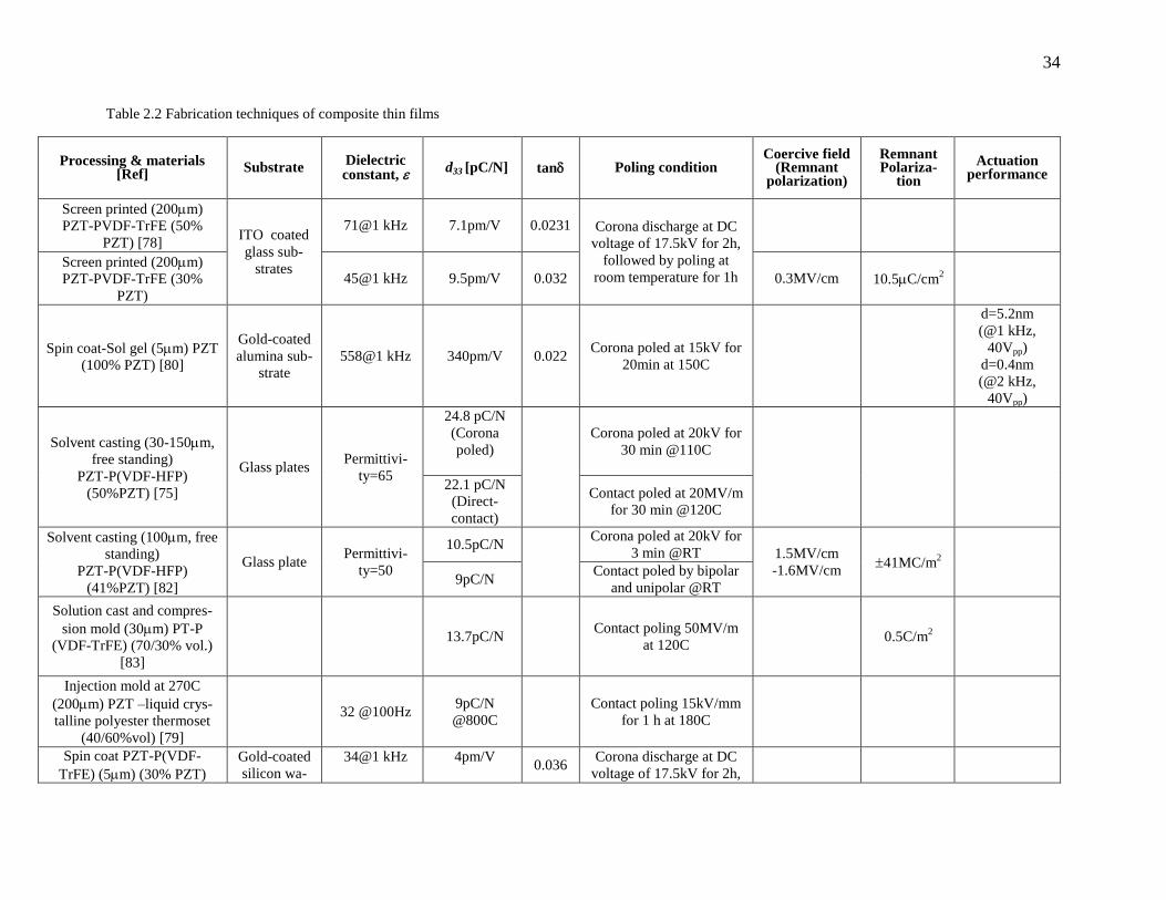
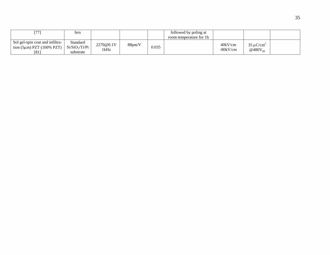
Table 2.2 Fabrication techniques of composite thin films ................................................ 34
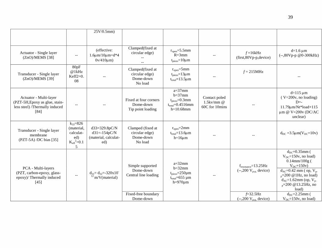
Table 2.3: Fabrication techniques and performances of dome-shaped piezoelectric
devices............................................................................................................................... 38
Table 3.1: Physical, dielectric and piezoelectric properties of the materials used in the
fabrication of piezoelectric dome shaped structures. The values for the PZT are for bulk
PZT as published by APC International. The values for the DEGBA were determined
from an epoxy dome structure Fabricated using the same steps as defined herein with 0%
PZT. .................................................................................................................................. 44
Table 4.1 Measurement of viscosity ................................................................................. 61
Table 4.2 Comparison between corona poled and contact poled data in 70% PZT ......... 65
Table 4.3 Spin-speed/time profile study ........................................................................... 78
Table 4.4 Deposition techniques study's results ............................................................... 79

1
Chapter 1
Introduction
1.1 Background
Piezoelectric materials generate electric charges when they are subjected to mechanical
stress and vice versa [1-3]. Piezoelectric ceramics are widely employed as sensors and
actuators because of their ideal electromechanical properties [4-8]. Homogenous ceramic
piezoelectric actuators are typically simple in structure and design (disks, rings, plates
and cylinders [9]) and are highly reliable with cycle lives that can range from 103 to 10
6
[6, 10-12]; render large actuation forces (dynamic force = 128 N @ 120 Volts and static
force = 275N to 375N @100 Volts[13]) and high sensitivity
(-1.3∙10-4
to -1.3∙10-3
m2∙kg-1
∙λ-1
[14]) rapid response times (response times can range
from 5μsec to 50μsec [15]); and consume low power during operation (power ranges 100
W to 500 mW [16-18]) [8]. Despite these advantages, piezoelectric ceramics are brittle
in nature (ultimate strength < 100 MPa [19, 20]) and have low fracture toughness
(0.5~2.0MPa∙√m)[19]. The intrinsic material characteristics limit their operational strains
(lead zirconate titanate (PZT)~0.1% at 10kV/cm [4]), operational loading frequency, cy-
cle life and compatibility to applications that require complex shapes. These poor me-
chanical properties limit their effective and efficient application to devices such as; hy-
drophones[21, 22], static and vibration based energy harvesting devices[23-25], surgical
tactile sensors [8, 26, 27] and synthetic jet actuators[28]. Devices such as these are typi-
cally fabricated into complex shapes and structures for enhanced sensitivity, long cycle
life reliability and increased displacement and loading. Piezoelectric polymers, such as

2
polyvinylidene fluoride (PVDF) are flexible, lightweight and have low acoustic and me-
chanical impedance, but suffer from low piezoelectric properties (d31~6-28 pC/N) [29,
30]. Hence, researchers have begun to investigate piezoelectric composite materials.
Composite piezoelectric materials (CPM), such as 0-3 piezoelectric composites
are a category of CPM that has been extensively studied ([3, 31]). Piezoelectric compo-
sites with 0-3 connectivity are fabricated so that active piezoelectric filler particles are
uniformly distributed within a matrix, where the matrix is self-connected throughout the
material while the piezoelectric particles are not self-connected throughout the material.
Piezoelectric composites are of interest for many reasons. They offer improved mechani-
cal strength and toughness. For example, P(VDFTrFE)/Ca-modified PbTiO3 composite
with 50% volume fraction of ceramic has an elastic stiffness coefficient, C33D
of a 34.5-
40.8 GPa @ 20 MHz [32] juxtapose to PZT whose elastic stiffness is 13.6 GPa [33]. Pie-
zoelectric composites can also be fabricated to have high hydrostatic performance); can
offer better electromechanical coupling with host structures; can be less difficult to fabri-
cate and are compatible to mass production techniques.
Over the past decade interest in the dome and curved shaped piezoelectric devices
has increased because these structures demonstrate higher deformation (PZT~25.3% at
2.54kv/cm [34]) and electromechanical conversion accuracy (mechanical coupling factor,
PZT-5A, Keff~38%[35]) in comparison to planar actuators [36-39]. These materials are
typically used in transducers[37, 40], hydrophones[21, 22], actuators[5, 27, 31, 36, 41-
48] and sensors[49], but are limited in their functionality and performance due to the
electrical/mechanical properties of the materials used. Also, the control of dome height
during the manufacture of the structure remains a challenge because most methods em-

3
ploy the thermal mismatch effect to induce dome shape, which requires more expensive
processing parameters, e.g. high temperatures [43, 50, 51] and vacuum [50] .
1.2 Research Goals and Hypotheses
In this work, dome-shaped 0-3 piezoelectric composites comprised of lead zirconate ti-
tanate (Pb(ZrxTi1-x)O3 (0≤x≤1)) and epoxy (PZT volume fraction ranged from 0.1 to 0.7)
were fabricated using a combination mix, spin coat and cast method. The influences of
the viscosity (composite mixture before the spin coat process), the spin-coating
time/speed profiles and poling voltage, on the effective composite piezoelectric and die-
lectric properties, were investigated. This work builds upon the prior work of Banerjee et
al. and Wei [31], where piezoelectric dome composites were fabricated and analyzed.
These devices suffered from the high agglomeration of PZT particles, ununiformed sur-
face morphology and a density of air bubbles which resulted in low piezoelectric coeffi-
cients and dielectric properties. The goal of this work was to isolate specific processing
parameters that would enhance the piezoelectric and dielectric properties of the dome-
shaped structures to make the devices more amenable to actuator applications.
Three research hypotheses were developed to address some of the challenges of
the previous devices. The first hypothesis is that the spin speed and the length of time of
the coating intervals influenced the dielectric and piezoelectric properties of the compo-
sites and that changes in the deposition process time intervals and speed would render
different values of dielectric and piezoelectric properties. To test this hypothesis, sam-
ples deposited by four separated time/speed profiles, were fabricated and analyzed. This
study was done on samples that had 0.50 volume fraction of PZT. The second hypothesis
is that the composite dome structures will render higher piezoelectric properties if a Co-

4
rona polarization process were implemented instead of a contact parallel-plate process.
The third hypothesis is that composite gels that there were within an optimal viscosity
range prior to deposition would lead to films of uniform thickness and films with higher
longitudinal piezoelectric strain values.
1.3 Research Materials and Methodology
The materials of interest are PZT-epoxy composites, where the volume fraction of PZT
was varied from 0% to 70% (increments of 10% for each volume fraction). The materials
used in the original study and this work were maintained. The lead zirconate titanate used
is called PZT – 855 and the two-part epoxy is DGEBA, EpofixTM Cold-setting embed-
ding Resin (purchased from APC International and Electron Microscopy Sciences, re-
spectively).
The samples are fabricated using a combination of sol-gel and spin-coat deposi-
tion process where devices were polarized using contact and corona methods. The pie-
zoelectric strain coefficients d33 and d31 were measured with a Piezo-meter @ 110Hz.
The electrically induced displacement was measured by KEYENCE LG-10 interferome-
ter. The dielectric impedance, phase angle, capacitance, conductance, resistance and die-
lectric loss (tan ) were measured as a function of frequency (2kHz to 20 MHz) on sam-
ples that used aluminum tape as the top electrode. The dielectric constant, conductivity
and resistivity were calculated from the capacitance, conductance, resistance and geome-
try of the samples, respectively. The P-E hysteresis loops of PZT-Epoxy 0-3 two-phase
dome shaped piezoelectric structure were measured under 750kv and 1000kv by Preci-
sion Ferroelectric Tester from Radiant technology Inc. The surface morphology and par-

5
ticle distribution were examined with the aid of Zeiss Sigma Field Emission Scanning
Electron Microscope(SEM) and Energy Dispersive X-Ray Spectroscopy(EDS).
1.4 Overview of the organization of the thesis
This thesis is organized in the following manner. In chapter 1, the research goals and hy-
potheses are introduced. In Chapter 2, basic definitions for dielectric, piezoelectric and
ferroelectric materials, polarization and composite connectivity are provided. In addition,
a comprehensive review of the state of the art in the literature on piezoelectric thin films
and piezoelectric dome/curved structures is presented in Chapter 2. In Chapter 3, the ex-
perimental methodology for fabrication of the devices and the analyses are presented. In
particular, studies that examine the influence of the time/speed profiles of spin-coating,
polarization technique and viscosity are presented. In Chapter 4, the results of the studies
are presented along with an interrogation and discussion of the mechanisms leading to the
results. Finally in Chapter 5, the conclusions of the thesis are presented.

6
Chapter 2
Definitions, Fundamental Concepts and Literature Review
2.1 Dielectric Materials
Dielectric materials are a type of electrical insulator, where when an external electric
field is applied the positive and negative charge centers separate. Under the influence of
an external electric potential, the positive charges are attracted to the surface with lower
electric potential, and the negative charges are attracted to the surface with higher electric
potential. The charges accumulate on the surfaces of dielectric material to resist the ex-
ternal electric field, which results in the alignment of the material dipoles in the direction
of the applied electric field.
Figure 2.1: (A) Normal state of dielectric material, the dipoles are randomly oriented. (B) Under the influ-
ence of external electric field, the dipoles are aligned.
Dielectric materials can be divided into two major groups [52]: Polar and Non-polar die-
lectrics. Polar dielectrics, such as NH3, HCl and H2O are composed of two or more atoms
(A) (B)

7
that have separated positive and negative charge centers. Dielectric polar molecules have
permanent polarizations. Without the presence of an electric field, these dipoles are ori-
ented randomly, so even though they possess permanent dipole moments - the overall po-
larization of the material is zero. The dipoles can be reoriented into a specific direction
with the application of an external electric field. Non-polar dielectrics, such as H2 and
O2, have coincidental positive and negative charge centers, and therefore do not possess a
permanent dipole moment. A dipole moment can be induced in non-polar dielectrics,
with the application of an external electric field, i.e. the separation of the positive and
negative charge centers with the application of an external electric force. Polar and non-
polar dielectrics such as HCl and H2 are shown in Figure 2.2.
Figure 2.2: (A) Example for non-polar dielectrics, no permanent dipole moments possessed. (B) Example
for polar dielectrics, permanent dipole moments are randomly oriented.

8
2.2 Polarization
Polarization describes the density of permanent or induced electric dipole moments with-
in a material and is expressed as a vector that points in the direction of the alignment of
the dipoles within the material. It is an important physical property that distinguishes in-
sulators, dielectrics and conductors from one another. The polarization of a material is
the summation of dipole moments per unit volume of the material. An electric dipole is a
pair of separated positive and negative electric charges as shown in Figure 2.3.
Figure 2.3: Schematic of a dipole pair that is comprised of a positive and negative charged centers.
The dipole moment, �⃗� of a single pair of charges could be calculated from vector
equation 2.1,
𝑝 = 𝑞 ∙ 𝑟 [53], 2.1
where �⃗� is dipole moment (unit, Coulomb-meter), 𝑞 is the electricity processed by a sin-
gle charge (Coulombs) and 𝑟 is the distance between the positive and negative charges
(unit, m). The polarization of can be calculated by vector equation 2.2,
�⃗⃗� =∑ 𝑝𝑖⃗⃗⃗⃗⃗
𝑉 [54], 2.2
where �⃗⃗� is polarization, 𝑝𝑖⃗⃗⃗ ⃗ is dipole moment of the ith
pair of charges per unit volume, 𝑉.
A material may be polarized via four mechanisms: electronic polarization, ionic
polarization, orientation polarization and space charge polarization. Electronic polariza-
tion occurs when an external electric field is applied to a material and the electrons dis-
place relative to their nuclei. In this case, the center of the electron clouds displace in the

9
direction of lower electric potential. An illustration of the electric polarization of H2 is
provided in Figure 2.4.
Figure 2.4: Mechanisms of electronic polarization. In (A) there is no external electric field applied. Thus,
there is no permanent dipole moment. In (B) an external electric field is applied, and dipole moments are
induced, which results in the alignment of the dipoles within the material.
The second type of polarization, ionic polarization is the most common. Ionic po-
larization occurs when the centers of positive and negative charges (i.e. cations and ani-
ons) within molecules are reoriented after the application of an electric field. This re-
orientation is in the direction of the applied electric field. An example of the ionic polari-
zation of sodium chloride (NaCl) is depicted in Figure 2.5.
10
Figure 2.5: Mechanism of ionic polarization: (A) Without the presence of the external electric field, posi-
tive and negative’s gravity center are coincident, there is no permanent dipole moments. (B) With the ex-
ternally applied electric field, gravity centers of positive and negative charges are separated; dipole mo-
ments are induced and aligned.
When molecules themselves possess a permanent dipole moment, the applied
electric field will reorient the molecules so that the permanent dipole moment will be in
the opposite direction of the external electric field, this is called orientation polarization.
An example of orientation polarization is shown in Figure 2.6.
Figure 2.6: Mechanism of orientation polarization: (A) Permanent dipole moments are facing different di-
rections, over all polarization is zero. (B) With the externally applied electric field, permanent dipole mo-
ments are aligned.
The forth source of polarization is space charge polarization, which happens when
the electrons or the ions migrate larger distances within more conductive phases and ac-
cumulate on the surfaces of more resistive phases [54] when subjected to an external
electric field. The mechanism of space charge polarization is shown in Figure 2.7.

11
Figure 2.7: Mechanism of space charge polarization: (A) Without external electric field, the ions are mixed
up. (B) At the presence of external electric field, the ions could travel larger distance inside the material.
Dielectric materials possess at least one of the four types of polarization mecha-
nisms mentioned above. The degree of polarization within a material is a function of the
frequency of the alternating electric field [52].
Dielectric materials store energy in terms of polarization. The relative complex
permittivity is an indicator of the effectiveness of the dielectric material in storing energy
in comparison to vacuum. The responses of dielectric material under the influences of an
alternating current (AC) are very closely related to the frequency of the electric field. The
relationship between the complex permittivity and relative complex permittivity is ex-
pressed in equation 2.3,
휀𝑟 = 휀휀0⁄ , 2.3
where 휀𝑟 is relative complex permittivity, 휀0 is the dielectric constant of vacuum
(8.85410-12
F/m ) and 휀 is the overall complex permittivity of the occupied space. The
relative complex permittivity could be further expressed as equation 2.4, where 휀𝑟′ is the
real part of relative complex permittivity, and 휀𝑟" is the imaginary part of relative com-
plex permittivity. The relationship between the real and the imaginary parts of the permit-

12
tivity are shown in Figure 2.8. Both the real and imaginary parts of the complex permit-
tivity vary depending on the given frequency. The real part of the complex permittivity
(i.e. 휀𝑟′) is a measure of how much energy has been stored in the dielectric material (re-
ferred as dielectric constant). The imaginary part of complex permittivity (i.e. 휀𝑟") is a
measure of how dissipative or lossy the material is in facing the alternative electric field.
The dissipation factor or loss tangent is a measurement of how dissipative the material is
compare to its ability to store energy [55]. could be shown in equation 2.4.
Figure 2.8: Real part and imaginary part of relative complex permittivity
tan 𝛿 =
휀𝑟"
휀𝑟′⁄ , 2.4
Given the frequency of the AC field, the real part of the complex permittivity
(mostly referred as dielectric constant) could be calculated through polarization.
Polarization describes how the charges are distributed inside the material, in or-
der to describe the matter without the effect of vacuum, the electric displacement field,
denoted as �⃗⃗⃗� is introduced. Electric displacement field accounts for the effects of free
and bound charge within materials. The relation of �⃗⃗⃗� , �⃗⃗� and dielectric constant of vacu-
um could be presented as vector equation 2.5,

13
�⃗⃗⃗� = �⃗⃗� + 휀0�⃗⃗� [54], 2.5
where �⃗⃗� is polarization, 휀0 is dielectric constant of vacuum and �⃗⃗� is applied electric field.
As the polarization under given electric field is a property of the material itself, so the
electric displacement field �⃗⃗⃗� could be express as equation 2.6as well,
�⃗⃗⃗� = 휀𝑟휀0�⃗⃗� [54], 2.6
where 휀𝑟 is dielectric constant of the material of interest. The mathematical relationship
between 휀𝑟 and �⃗⃗� could be expressed in 2.7.
𝑃 = (휀𝑟 − 1)휀0𝐸 [54], 2.7
Dielectric constant, also referred as real part of the relative complex permittivity,
is the indicator of how effective of the material behaves as a capacitor, which cannot be
measured directly. Usually the capacitance, which accounts for the ability to store charg-
es, area and the thickness of the specimen are measured, and the dielectric constant may
be subsequently calculated as a function of Capacitance using equation 2.8.
휀𝑟 =
𝐶∙𝑑
𝐴∙𝜀0, 2.8
where, 휀𝑟 is the relative dielectric constant, 휀0 is dielectric constant of vacuum (휀0 ≈
8.854 × 10⁻¹²F ∙ m−1), C is capacitance, A is area and d is the thickness of the piezoe-
lectric composite layer.
2.3 Piezoelectric material
Piezoelectric materials are a class of dielectrics, that can not only be polarized by an elec-
tric field but also a mechanical stress [52]. This special property arises from the crystal
structure of piezoelectric material. Some of the piezoelectric materials have permanent
dipole moments; some of them have their positive and negative charge center coinci-

14
dence. Due to piezoelectric materials’ natural non-centrosymmetric crystal structure,
when stress is applied, the distortion of the crystal structure will further separate or in-
duce the separation of positive and negative charge centers, this phenomenon is shown in
Figure 2.9.
Figure 2.9: Polarization induced by mechanical stress. (A) Without applying the mechanical stress, positive
and negative charge centers are in coincidence. (B) After the mechanical stress is applied, the dipole mo-
ment is induced.
There are many materials in our everyday life that have piezoelectricity, such as
quarts and bones. Polarization is developed when a piezoelectric material is subjected to
mechanical stress. Similarly, the converse piezoelectric effect occurs when an external
electric field is applied to the material and it develops a strain in response to the applied
stress. Both piezoelectric and converse piezoelectric effects are shown in Figure 2.10.
15
Figure 2.10: Schematic representation of piezoelectric and converse piezoelectric effect. (A) The material
after polarization, the polarization direction sis shown in the figure. (B)&(C) explain piezoelectric effect:
the polarized material is under stress, and produces voltage. (D)&(E) denotes converse piezoelectric effect,
when polarized material is subjected to external electric field the strains are induced[9].
Within the 7 crystal system, there are 32 points groups in total that have the pos-
sible combinations of symmetries, 11 of them are centrosymmetric point groups, 21 of
them are non-centrosymmetric groups. Since Neumann's Principle[56] is applied, the pie-
zoelectricity is limited to materials have non-centrosymmetric structures. Point group 432
is special because the dipole moments generated along axis <111> cancels each other,
left this point group similar to centrosymmetric point groups. However, the non-
centrosymmetric structure is only necessary to piezoelectricity but not sufficient, as only
a few thousand materials exhibit meaningful piezoelectric effect compared to several
hundred thousand materials with non- centrosymmetric structures.
The critical measurement of piezoelectricity are the piezoelectric coefficients, e.g
the piezoelectric charge coefficients. The linear piezoelectric constitutive equations for
the converse and direct piezoelectric effects are expressed in equation 2.9 and equation
2.10, respectively,

16
𝑆𝑖𝑗 = 𝑑𝑘𝑖𝑗 ∙ 𝐸𝑘 (Converse piezoelectric effect), 2.9
𝐷𝑘 = 𝑑𝑘𝑖𝑗 ∙ 𝛿𝑖𝑗 (Piezoelectric effect), 2.10
where 𝑑𝑘𝑖𝑗 is the piezoelectric charge coefficient tensor, 𝑆𝑖𝑗 is corresponding strain ten-
sor, and 𝛿𝑖𝑗 is the stress tensor, where 𝑖, 𝑗 = 1,2,3. The first index indicates the direction
of polarization, the second index denotes the normal to the surface where the stress acts,
and the third index is the actual direction on specific surface. As 𝐸𝑘 and 𝐷𝑘 are both first
order tensors, and 𝑆𝑖𝑗 and 𝛿𝑖𝑗 are both second order tensors, 𝑑𝑘𝑖𝑗 is the third order tensor,
which have 33=27 elements in total. Owing to the symmetric property of strain and stress
tensor (𝑆𝑖𝑗 = 𝑆𝑗𝑖, 𝛿𝑖𝑗 = 𝛿𝑗𝑖) so 𝑑𝑘𝑖𝑗 = 𝑑𝑘𝑖𝑗 and the total number of piezoelectric coeffi-
cients reduces to 18 [52].
The lowest symmetry point group is point group 1, from the triclinic crystal sys-
tem, which only has 1 fold of rotation. So the crystals in this point group will not have
further reduction in the number of piezoelectric charge coefficients like other point
groups who have more symmetry elements. The piezoelectric coefficient tensor are ex-
pressed in equations 2.11, 2.12 and 2.13,
𝑑1𝑗𝑘 = [
𝑑111 𝑑112 𝑑113
𝑑112 𝑑122 𝑑123
𝑑113 𝑑123 𝑑133
], 2.11
𝑑2𝑗𝑘 = [
𝑑211 𝑑212 𝑑213
𝑑212 𝑑222 𝑑223
𝑑213 𝑑223 𝑑233
], 2.12
𝑑3𝑗𝑘 = [
𝑑311 𝑑312 𝑑313
𝑑312 𝑑322 𝑑323
𝑑313 𝑑323 𝑑333
]. 2.13
As we can see from those equations, all three tensors are symmetric, so the last
two indexes may be rearranged as shown in Table 2.1.

17
Table 2.1 Index transformation
11 1
22 2
33 3
23/32 4
31/13 5
12/21 6
Then after rearranging, the new piezoelectric charge coefficient tensor may be ex-
pressed as,
𝑑 = [
𝑑11
𝑑21
𝑑31
𝑑12
𝑑22
𝑑32
𝑑13
𝑑23
𝑑33
𝑑14
𝑑24
𝑑34
𝑑15
𝑑25
𝑑35
𝑑16
𝑑26
𝑑36
]. 2.14
The crystal structures are centrosymmetric, by multiplying inverse transformation
matrix [−1 0 00 −1 00 0 −1
] on the left, the piezoelectric charge coefficient tensor will be– 𝑑,
and at the same time Neumann's Principle requires that 𝑑 =– 𝑑, all elements in piezoelec-
tric charge coefficient tensor will be cancelled. So non-centrosymmetric is necessary for
piezoelectricity. The increasing number of symmetries possessed by crystal structure re-
duces the number of remaining piezoelectric charge coefficient elements. Piezoelectric
charge coefficient d33 and d31 are most commonly measured. They are often measured as
charges accumulated when subjected to vibrations. The frequency of vibration should be
within 25-300Hz[54]. For piezoelectric charge coefficients mentioned here, the polariza-
tion direction is both in 3rd direction, the stress applied when measuring d33 is also in 3rd
direction, however, the stress applied when measuring d31 is in 1st direction. The direc-
tions of polarization and stress for both cases are indicated in Figure 2.11 and Figure
2.12.
18
Figure 2.11: Illustration of d33 measurement. (A)Polarized sample (B) The measurement of d33, the meas-
urement tube would apply the vibration and take the voltage reading at the same time.
In Figure 2.11, in measuring the d33, the polarization direction is in 3rd direction,
when stress in terms of vibration is applied also in 3rd
direction, the measurement tube
will measure the polarization along the same direction.
Figure 2.12: Illustration of d31 measurement

19
In Figure 2.12, to measure d31, the polarization direction is still in the 3rd direction;
however, the vibration is applied in 1 direction. Once the measurement started, the tubes
will measure the polarization along the 3rd direction.
2.4 Ferroelectrics
Ferroelectrics are crystals with a spontaneous polarization that can be switched from one
orientation to another by an externally applied electric field[52]. All ferroelectrics are pi-
ezoelectric and ferroelectrics are different from normal piezoelectric materials. First, they
possess spontaneous polarization, and their polarization can be switched from one orien-
tation to another when an external electric field is applied. Second, the phase transition
can also affect the spontaneous polarization, when temperature keeps increasing, the
crystal structure becomes more symmetric. Beyond a critical temperature called the Curie
temperature, the current crystal structure will become a centrosymmetric cubic shape
structure, which is the temperature at which a ferroelectric material will loose its sponta-
neous polarization. When the temperature is reduced these materials experience a phase
transaction to a lower symmetric structure, and the spontaneous polarization emerges
again. Third, all ferroelectric materials have domains, as when they are cooled from a
higher temperature above the Curie temperature, the permanent dipole moments are gen-
erated and aligned in different directions. The units aligned in the same direction will
form a domain, and will be separated from adjacent domains whose polarization is in a
different direction. These properties come from their crystal structures.
The most important property of ferroelectric is reversible spontaneous polariza-
tion, which lead to the Polarization-Electric field (P-E) hysteresis loop. P-E hysteresis
loop, as its name indicates, is measuring the polarization accumulated versus the increas-

20
ing strength of externally applied electric field. Dielectrics except ferroelectrics have a
linear polarization-electric field relation as shown in Figure 2.13, where when the exter-
nal electric field is removed, the polarization will no longer exist.
Figure 2.13: P-E relation of normal dielectrics
Ferroelectrics’ P-E relations could be presented as a hysteresis loop, as shown in
Figure 2.14. The actual P-E hysteresis loop includes line AB, BC and CD, however, we
could only observe lines of AB, BB’, CC’ and CD[57].
Figure 2.14: Hysteresis loop pf ferroelectrics[46]

21
The whole hysteresis loop is explained more clearly in Figure 2.15. Even though
ferroelectrics have spontaneous polarization in their initial state, their overall net polari-
zation is equal to zero because of the existence of multiple domains with different spon-
taneous polarization directions. Once the external electric field is applied, the polarization
is increased with the strength of the electric field until saturated; this is OB line in Figure
2.15. The saturation point of polarization means that all possible switchable domains are
aligned in the direction of the electric field. Increasing the strength of the electric field
beyond this point will not increase polarization anymore. As shown in this figure, the
gradual reduction in the external electric field to zero results in a net overall polarization
called the remnant polarization, which is denoted as Pr. The higher the remnant polariza-
tion value, the more domains of spontaneous polarization that are aligned in the electric
field’s direction. If the electric field continues to increase in the opposite direction, the
polarization will be compensated eventually. The strength of the external applied electric
field applied required to achieve zero polarization is called coercive field, denoted as Ec.
Ec indicates the resistance to reverse the direction of the polarization. This process is
shown in Figure 2.15 as line CF. If the external electric filed increases further, the ferroe-
lectrics would be polarized in the opposite direction until saturated, which is shown as
line FG. Then the line GHB is describing the similar phenomenon just in opposite direc-
tion.

22
Figure 2.15: Hysteresis loop of ferroelectrics with original polarizing path[57]
Ferroelectric materials exist in different conditions such as single crystal, poly-
crystalline ceramic and fine grain ceramic will have hysteresis loop in different
shape[57]. In measuring hysteresis loops, programmed changing electric field is applied,
and the polarization information will be collected.
There are different types of piezoelectric such as Bi-layer structured systems,
Tungsten bronze structures and most common one--perovskite structures. Most ferroelec-
trics adopt the ABO3 perovskite structure, and we will mainly focus on this group of fer-
roelectrics. General chemical formula of materials with perovskite structure is ABO3, de-
pending on the size of A atom and B atoms (there could be more than one type of B at-
oms), they could mostly belong to tetragonal, orthorhombic, rhombohedral and cubic
crystal systems. Along the increasing of the temperature, the structure will gradually gain

23
more symmetry element until reach the cubic shape. The tetragonal perovskite structure
below Curie temperature is shown in Figure 2.16, blue bigger atoms are A2+
, red big at-
oms are O2+
and the smallest black atom is B4+
. If we take PZT as an example, the blue
atoms will be Pb2+
, the red big atoms will be O2+
and the smallest black atom will be
Zr4+
. From Figure 2.16 we could also see that the positive and negative charge centers are
not coincident, this leaves the ferroelectrics permanent dipole moment.
Figure 2.16: Tetragonal perovskite structure below Curie temperature[9]
When the temperature is increased beyond Curie temperature, the perovskite
structure will experience a phase change and become centrosymmetric. The crystal struc-
ture above Curie temperature is shown in Figure 2.17, the positive and negative charge
centers are at the same place, and piezoelectricity is lost.
Figure 2.17: Cubic perovskite structures above Curie temperature[9]

24
As domains with polarization in different direction, before ferroelectrics present
piezoelectricity, we need to apply external DC electric file to align dipoles in favorable
direction. Aligning spontaneous polarization in one favorable direction by applying ex-
ternal DC electric field is called poling. Depending on different crystal structure, there
could be many polarization directions, for examples, rhombohedral crystal class could
have as many as 8 polarizations directions, orthorhombic crystal class could have 12 po-
larizations directions, and tetragonal crystal structure will have 6 polarizations directions.
When crystals are cooled from Curie temperature, multiple domains are formed, and do-
mains next to each other develop spontaneous polarizations in different directions, so the
overall net polarization is zero. By applying DC electric field, mostly two effects could
be observed: (1) Upon applying the electric field, the spontaneous polarization could be
switched, as mentioned above that all different crystal systems have more than one polar-
ization direction. (2) The externally applied electric field would induce domain wall mo-
tion. The applied electric field supply the energy that B4+
requires to jump from one equi-
librium state to another, i.e. flip the polarization to the opposite direction by B4+
atom
moving correspondingly. The elevated temperature is also required to help overcome the
energy barrier.
2.5 Polarization Techniques
2.5.1 Parallel Plate Contact Poling
As sufficient polarization is important for ferroelectrics, different poling techniques are
developed. Conventional contact poling, as shown Figure 2.18, usually employs two met-
al electrodes connected to a DC voltage source, and sample will be sandwiched in be-

25
tween, the two electrodes will direction contact the surface of the sample, and the whole
set up is bath in heated silicon oil.
Figure 2.18: Sketch of conventional contact poling set-up
During the fabrication, deficient points and voids would commonly occur on
samples, when poled by conventional contact poling, once the charges find one pathway
to go through, not only the electric field over that deficient point will be lost but the
whole electric field will be vanished, so the sample will not be properly poled, this is
called dielectric breakdown in poling process. So contact poling requires high quality of
samples and also possibly could not offer electric field enough to sufficiently polarize
samples.
2.5.2 Corona Poling
Corona poling, as indicated by its name, employs corona charges to create electric field.
The scheme figure of corona poling set up is shown in Figure 2.19. The sample will be
heated on a heat source, and only contact with ground. The needle right on top of the

26
sample will be connected to high voltage. One turned on, the tip of the needle will ionize
surrounding air, and the electric field generated by ionized air will align the dipoles.
Figure 2.19: Sketch of corona poling set-up
In corona poling process, the deficient points where charges could leak through, will
not affect the overall electric field except the deficient point itself since the ‘top elec-
trodes’ are ionized air. Thus, by employing corona poling much higher poling voltage can
be achieved.
2.6 Composite Materials
According to the broadest definition, a composite is any material consisting of two or
more distinct phases[58]. Composites viewed as an intermediate, could inherit the ad-
vantages of all materials have been employed. Composite piezoelectric materials (CPM)
possess several characteristics that distinguish them from their single-phase ceramic
counterparts: few spurious modes (less noise associated with resonant modes), high com-

27
pliance/flexibility (less brittle), and flexibility in processing - moldable (can be easily
fabricated into synclastic and anticlastic shapes).
Composite’s electromechanical and all other properties are based on arrangement
of the phases comprising the composites[59]. The connectivity was first brought up by
Skinner[60] and Newnham[61], based on in how many directions the material is self-
connected. For example, if material A is embedded in material B, if A is self-connected
in 3 directions then A has connectivity of 3, and if material B only self-connected in 1
direction then B has connectivity of 1, the composite will be called as A-B 3-1 two-phase
composite. Even with more than two phases, the expressions should follow the same
fashion.
For two-phase composite, there are 10 established connectivity patterns, such as
(0-0), (0-1), (0-2), (0-3), (1-1), (1-2), (2-2), (1-3), (2-3), and (3-3) [59]. The patterns
could be illustrated better by Figure 2.20.

28
Figure 2.20: Here shows 10 connectivity pattern families, especially in {0-1}, {0-2}, {0-3}, {1-2},{1-3}
and {2-3} families, each of them include 2 connectivity patterns, which makes total number of connectivity
pattern16[60].
Based on connectivity concept, lots of piezoelectric/polymer has been devel-
oped[60, 61], such as particles in a polymer (0-3), ceramic rods in a polymer (1-3), diced
composite (1-3), ceramic air composite (3-0), sheet composite (2-2), ladder composite (3-

29
3), more composites developed are shown in Figure 2.21.
Figure 2.21: Schematics of typical piezoelectric ceramic composite structures [23]
As desirable as piezoelectric, their brittle nature limits them from being suitable
for applications that require flexibility and particular shapes. Ferroelectric composites,
embedding ferroelectric into matrixes, offer improved mechanical properties compared to
ferroelectric ceramics, and inherit the excellent electromechanical and dielectric proper-
ties.
Embedding in matrix with different properties opens many opportunities for
CPMs in varied applications. Cement-based piezoelectric composites, could be used as
sensors and transducers in buildings with smart structures[62]. Polymer-based CPMs are
well suitable for actuator and sensor applications. Polymer-based CPMs have electrome-
chanical coupling factors (Kt~60%-92%[63]) that are comparable and higher to single-
phase ceramic (K33~40%-94%[59]) and polymer piezoelectric materials (Kt~11%-30%

30
[59, 64]), respectively. CPMs also demonstrate enhanced fracture toughness and high
mechanical shock resistance, which renders them amenable to high quality thin and thick
film applications[59].
Among all connectivity patterns introduced above, 0-3 piezoelectric composite
standout as one of the easiest to produce and highly compatible to massive production. In
0-3 composite, the piezoelectric ceramic powders are not self-connected in any direction
while the host material (i.e. polymer) is three-dimensional connected (Figure 2.20). Pol-
ymer based 0-3 composite offers good compatibility with various acoustic couplings such
as castor oil[65]. Moreover, its properties are independent of pressure and frequency.
Polymer based 0-3 composite are also attractive for power harvesting applications be-
cause of their ability to withstand large amounts of strain[1]. The larger the strain the de-
vice could take, the more energy could be possibly converted to electrical energy. The
polymer based piezoelectric composites are also suitable to transducers such as hydro-
phones[65-67], air sensors, vibration sensors, pressure and stress sensors[68], underwater
acoustic transducer[65] and medical diagnostic applications since they can be fabricated
in suitable thin and flexible forms to provide enhanced hydrostatic piezoelectric proper-
ties (low in dielectric constant) and improved acoustic impedance[69].
Despite all favorable features 0-3 composites could offer, the relatively low pie-
zoelectric coefficient limits this type of composites to be employed in applications need
larger electromechanical responses. This could be result from difficulties in evenly dis-
tributing the fillers into the matrix, especially in high concentrations. Voids might be cre-
ates during the process could contribute to lower the dielectric breakdown strength,
which may result in insufficient polarization for the ceramic phase. Besides all issues

31
mentioned above, as the nature of this composites (strong dielectrics embedded in weak
dielectrics) the severally distinction in ability to be polarized between two phases makes
the composite harder to be poled, as the electric filed will not come through the polymer
phase easily[59].
So in order to be compatible to wider applications, processing techniques to increase
homogeneity and poling techniques to improve polarizations of the active fillers are
needed. 2.7 Spin-coating process
Spin coating combined with sol-gel processing is one of most common techniques to ap-
ply thin films onto substrates, as the process could quickly and easily produce very uni-
form films from a few nano-meters to a few microns in thickness[70]. Spin coating was
first studied experimentally and analytically by Dietrich Meyerhofer [71]. This process
has been widely used in the manufacture of integrated circuits[70], microelectronic ap-
plications[72], optical devices , coating color in TV screens, magnetic storage disk, fabri-
cation of polymer and other Newtonian fluid based thin films[73].
Spin coating techniques use centrifugal force to dispense the solvent to a substrate.
Thickness and uniformity of the samples fabricated are sensitive to speed, gas conditions,
and rheology of concentrating, solidifying liquid[74]. The scheme of the spin coating
process could be shown in Figure 2.22.

32
Figure 2.22: Scheme of spin coating technique
2.8 Literature review
2.8.1 Composite piezoelectric materials
0-3 piezoelectric composites are a category of CPM that has been extensively studied (
[3, 31]). A summary of thin and thick film CPM piezoelectric and dielectric properties,
and fabrication methods is presented in Table 2.2. As indicated in Table 2.2, the majority
of the thick and thin composite films were fabricated using solvent casting[75, 76], spin-
coating[77], screen printing[78], mode injecting[79], combination of spin-coat and sol-

33
gel[80, 81]and combination of solvent casting and compressed mode methods for deposi-
tion of the precursor composite material onto planar substrates.
34
Table 2.2 Fabrication techniques of composite thin films
Processing & materials [Ref]
Substrate Dielectric constant,
d33 [pC/N] tan Poling condition Coercive field
(Remnant polarization)
Remnant Polariza-
tion
Actuation performance
Screen printed (200m)
PZT-PVDF-TrFE (50%
PZT) [78] ITO coated
glass sub-
strates
71@1 kHz 7.1pm/V 0.0231 Corona discharge at DC
voltage of 17.5kV for 2h,
followed by poling at
room temperature for 1h
Screen printed (200m)
PZT-PVDF-TrFE (30%
PZT)
45@1 kHz 9.5pm/V 0.032 0.3MV/cm 10.5C/cm2
Spin coat-Sol gel (5m) PZT
(100% PZT) [80]
Gold-coated
alumina sub-
strate
558@1 kHz 340pm/V 0.022 Corona poled at 15kV for
20min at 150C
d=5.2nm
(@1 kHz,
40Vpp)
d=0.4nm
(@2 kHz,
40Vpp)
Solvent casting (30-150m,
free standing)
PZT-P(VDF-HFP)
(50%PZT) [75]
Glass plates Permittivi-
ty=65
24.8 pC/N
(Corona
poled)
Corona poled at 20kV for
30 min @110C
22.1 pC/N
(Direct-
contact)
Contact poled at 20MV/m
for 30 min @120C
Solvent casting (100m, free
standing)
PZT-P(VDF-HFP)
(41%PZT) [82]
Glass plate Permittivi-
ty=50
10.5pC/N
Corona poled at 20kV for
3 min @RT 1.5MV/cm
-1.6MV/cm 41MC/m
2
9pC/N Contact poled by bipolar
and unipolar @RT
Solution cast and compres-
sion mold (30m) PT-P
(VDF-TrFE) (70/30% vol.)
[83]
13.7pC/N Contact poling 50MV/m
at 120C 0.5C/m
2
Injection mold at 270C
(200m) PZT –liquid crys-
talline polyester thermoset
(40/60%vol) [79]
32 @100Hz 9pC/N
@800C
Contact poling 15kV/mm
for 1 h at 180C
Spin coat PZT-P(VDF-
TrFE) (5m) (30% PZT)
Gold-coated
silicon wa-
34@1 kHz
4pm/V
0.036
Corona discharge at DC
voltage of 17.5kV for 2h,
35
[77] fers followed by poling at
room temperature for 1h
Sol gel-spin coat and infiltra-
tion (5m) PZT (100% PZT)
[81]
Standard
Si/SiO2/Ti/Pt
substrate
1kHz
88pm/V
0.035
40kV/cm
-80kV/cm 35 C/cm
2
@480Vpp
36
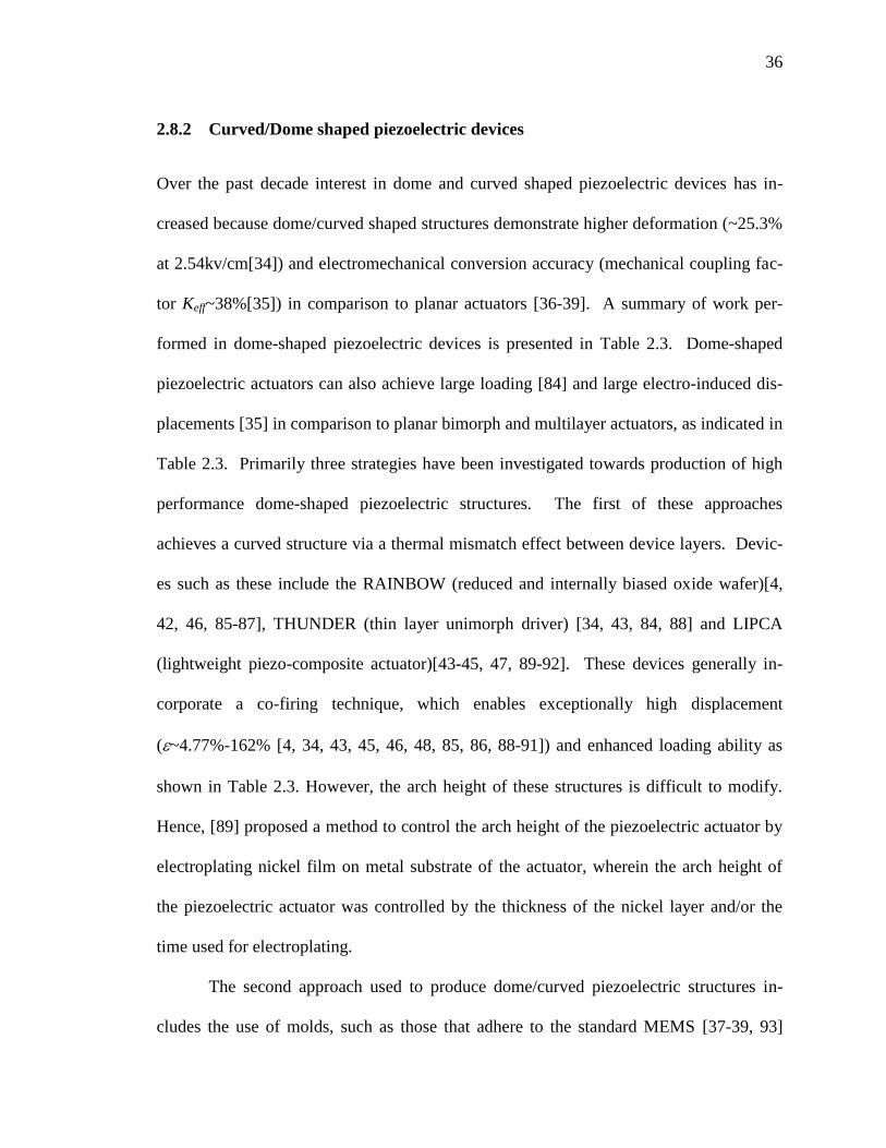
2.8.2 Curved/Dome shaped piezoelectric devices
Over the past decade interest in dome and curved shaped piezoelectric devices has in-
creased because dome/curved shaped structures demonstrate higher deformation (~25.3%
at 2.54kv/cm[34]) and electromechanical conversion accuracy (mechanical coupling fac-
tor Keff~38%[35]) in comparison to planar actuators [36-39]. A summary of work per-
formed in dome-shaped piezoelectric devices is presented in Table 2.3. Dome-shaped
piezoelectric actuators can also achieve large loading [84] and large electro-induced dis-
placements [35] in comparison to planar bimorph and multilayer actuators, as indicated in
Table 2.3. Primarily three strategies have been investigated towards production of high
performance dome-shaped piezoelectric structures. The first of these approaches
achieves a curved structure via a thermal mismatch effect between device layers. Devic-
es such as these include the RAINBOW (reduced and internally biased oxide wafer)[4,
42, 46, 85-87], THUNDER (thin layer unimorph driver) [34, 43, 84, 88] and LIPCA
(lightweight piezo-composite actuator)[43-45, 47, 89-92]. These devices generally in-
corporate a co-firing technique, which enables exceptionally high displacement
(~4.77%-162% [4, 34, 43, 45, 46, 48, 85, 86, 88-91]) and enhanced loading ability as
shown in Table 2.3. However, the arch height of these structures is difficult to modify.
Hence, [89] proposed a method to control the arch height of the piezoelectric actuator by
electroplating nickel film on metal substrate of the actuator, wherein the arch height of
the piezoelectric actuator was controlled by the thickness of the nickel layer and/or the
time used for electroplating.
The second approach used to produce dome/curved piezoelectric structures in-
cludes the use of molds, such as those that adhere to the standard MEMS [37-39, 93]

37
technology and powder injection molding (PIM) techniques [28, 36, 41]. These tech-
niques allowed for accurate control of the arch heights, and were compatible with batch
processing techniques.
The last category of fabrication methods investigated, employed a pressure differ-
ence [40, 49, 94] or DC bias [35] to achieve the dome-shaped structure. This approach
also enabled better control of the arch height and was compatible with batch processing
techniques. However, this approach was most appropriate for application to piezoelectric
thin film membranes.

38
Table 2.3: Fabrication techniques and performances of dome-shaped piezoelectric devices
Application - Processing &
materials [Ref]
/ tan /
keff
d33 /d31 BC/LC Geometry /layer
Poling Condi-
tions
Resonant Frequency
Max. Displacement
(Strain induced)
Unimorph
(PZT)/spin-coating
[This work]
56@110
Hz
d33=11.106 pC/N
d31=3.9 pC/N
(effective)
Corona poled
a@ 45kv/mm
(30min)
Actuator - Unimorph
(70% PZT)/spin-coating [31]
76.1
@110Hz
d33=425-500pC/N
(material)
d33=1.06 pC/N
d31=0.74 pC/N
(effective)
--
Dome-down
No-load
ropen=25.4mm
h=5.08 mm
ttotal=310m
Contact poled
2.2kv/mm @
75C for 15mins
-- --
Actuator - Three layers
(Nd2O3 & ZrO2 doped Ba-
TiO3)/co-firing [4]
2000-
3000
@1kHz /
Of the
order
0.01-0.02
d33=526pC/N
d31=325pC/N
(effective)
Unclamped
Dome-down
No load
ropen=0.28cm
hinner=0.04cm
ttotal=0.066cm
-- -- d=8m
( op ,Ep-p=20kv/cm
@0.1 Hz)
Actuator - Single layer
(0.04Pb(Sb0.5Nb0.5)O3–
0.46PbTiO3–0.5PbZrO3)/PIM
(powder injection mold) [36,
41]
k33T=195
0 / kp=0.7
(material)
d33=550pC/N
(material)
Clamped
Dome- horizontal
point load (weight of
the device only)
ropen=4.93mm
R=4.53mm
ttotal=0.4mm
Contact poled
2.5kv/mm @
150C in silicon
oil for 40mins
f=52kHz/51.4kHz/50.8kH
z
(first,60Vp-p, geometry
#1)
f=68.2kHz/61.6kHz
/98.3kHz
(first,60Vp-p, geometry
#2)
d=7.48m
(--,60Vp-p
@50kHz,10g)
LIPCA-C2 - Multi-layer
( PZT, Carbon/Epoxy,
Glass/Epoxy )/Thermally in-
duced [48]
d31= -190x10-12
m/V
d33= 390x10-12
m/V
(material)
Simply supported
Dome-down
No load
L=71mm/100mm
B=23mm/24mm
tpiezo=0.25mm
ttotal=0.62 mm
-- --
d=1.1552mm
(--,400Vp-p @1Hz, no
load)
Actuator - Single layer
(0.04Pb(Sb0.5Nb0.5)O3–
0.46PbTiO3–0.5PbZrO3)/PIM
(powder injection mold) [36]
ε= 1450 /
Kp= 0.7
(material)
d33=550pC/N
(material)
(effective:
700nm/0.5mm=d*
--
Dome-horizontal
Load unclear
ropen=8mm
R=10mm
ttotal=0.5mm
Contact poled
2.5kv/mm @
150C in silicon
oil for 40mins
f=0.5Hz
(first,50Vo-p, device)
d=700nm
(op,50Vo-p @1Hz-
0.33Hz)
39
25V/0.5mm)
Actuator - Single layer
(ZnO)/MEMS [38] --
(effective:
1.6m/10m=d*4
0v/410m)
Clamped(fixed at
circular edge)
--
--
ropen=5.5mm
R=3mm
tpiezo=10m
-- f =16kHz
(first,80Vp-p,device)
d=1.6 m
(--,80Vp-p @0-300kHz)
Transducer - Single layer
(ZnO)/MEMS [39]
80pF
@1kHz
Keff2=0.
08
--
Clamped(fixed at
circular edge)
Dome-down
No load
ropen=5mm
tpiezo=13m
ttotal=13.5m
--
f = 215MHz
--
Actuator - Multi-layer
(PZT-5H,Epoxy as glue, stain-
less steel) /Thermally induced
[84]
-- --
Fixed at four corners
Dome-down
Tip point loading
a=37mm
b=37mm
tpiezo=0.3mm
ttotal=0.4516mm
h=10.68mm
Contact poled
1.5kv/mm @
60C for 10mins
--
d=115 m
( V=200v, no loading)
D=-
11.79m/Nt*load+115
m @ V=200v (DC/AC
unclear)
Transducer - Single layer
membrane
(PZT-5A) /DC bias [35]
k33=826
(material,
calculat-
ed)
Keff2=0.1
5
d33=329.8pC/N
d31=-154pC/N
(material, calculat-
ed)
Clamped (fixed at
circular edge)
Dome-down
No load
ropen=2mm
ttotal=13.6m
h=16m
-- -- dDC =3.5m(VDC=10v)
PCA - Multi-layers
(PZT, carbon-epoxy, glass-
epoxy)/ Thermally induced
[45]
-- d31= d32=-320x10
-
12 m/V(material)
Simple supported
Dome-down
Central line loading
a=32mm
b=32mm
tpiezo=250µm
ttotal=655 µm
h=970µm
--
fresonance=13.25Hz
(--,200 Vp-p, device)
dDC=0.35mm (
VDC=150v, no load)
0.14mm/100g (
VDC=150v)
dAC=0.42 mm ( op, Vp-
p=200 @1Hz, no load)
dAC=1.62mm (op, Vp-
p=200 @13.25Hz, no
load)
Fixed-free boundary
Dome-down
f=32.5Hz
(--,200 Vp-p, device)
dDC=2.25mm (
VDC=150v, no load)

40
Central line loading 0.85mm/100g (
VDC=150v)
dAC=2.62mm ( op, Vp-
p=200 @1Hz, no load)
Actuator - Single layer
(PLZT 5.5/56/44
(La/Zr/Ti))/RAINBOW [85]
20.8nF /
2.5%
d33=312pC/N
(effective)
--
--
No-load
h=305µm
tpiezo=0.635mm
ttotal=635.5 µm
ropen=31.75mm
Three times of
coercive filed
strength
600-1000 Hz and 8-50
kHz (--,--,device)
They think this is bending
mode
d=125 µm
( DC: E=9.5kV/cm or
V=450v)
Actuator - Monolithic bilayer
composite(piezo:0.65PMN-
0.35PT; electrostrictive:
0.9PMN-0.1PT)/co-fire [86]
k33=2000
0
(material,
electro-
strictive)
k33=630
(material,
piezoe-
lectric)
d33=630pC/N
(material, piezoe-
lectric)
Unclamped
Dome-down
Tip-load
h=0.5mm
ropen=7.5mm
tpiezo=490µm
ttotal=986µ m
Contact poled
2.5kv/mm @
150C in silicon
oil for 10mins
--
d=15µm ( --,bipolar
10kV/cm @--, 0.5N)
d=14µm ( --,unipolar
10kV/cm @--, 0.5N)
Actuator - Single layer
(PLZT)/RAINBOW [87]
-- -- --
h=30µm
ropen=20mm
ttotal =tpiezo=0.5mm
-- -- --
Sensor - Multi-layers
(PZT-5A, Aluminum, LaRC-SI
adhesive film)/THUNDER
[34]
80-95nF
@(10-3
Hz-
100Hz)
--
Fixed at four corners
Dome-down
No-load
tpiezo=0.1778mm
ttotal=0.3937 mm
R=157.48mm
Re-poling:
420v for 5mins
fresonance=250Hz
(--,--, device)
They have stated that
resonance frequency is
independent on thickness
and driving voltage
dAC=0.642 mm ( --,Vp-
p=200 @1Hz & 10Hz,
no load)
LIPCA - Multi-layer
( PZT, Carbon/Epoxy ,Glass
/Epoxy )/ Thermally induced
[43]
-- d31= -176x10
-12
m/V(material)
Screw-fixed
Dome-down
Point load
L=71mm/100mm
B=23mm/24mm
tpiezo=0.1778mm
ttotal=0.25 mm
R=308.8mm
h=2.03mm
-- --
dAC=0.34mm (--,400Vp-p
@1Hz, no load)
0.17mm /1N(--,100Vp-p
@1Hz)
0.34mm /1N(--,200Vp-p
@1Hz)

41
LIPCA - Multi-layer
( PZT-3195HDs, Car-
bon/Epoxy UD(0),
Glass/Epoxy )/ Thermally in-
duced [89]
-- d31= -190x10
-12
m/V(material)
Simply-supported
--
Point load
L=71mm
B=23mm
tpiezo=0.25mm
ttotal=0.53mm
-- --
dAC=0.69mm (--, 400Vp-
p @1Hz, no load)
dDC=0.4mm
(VDC=200V, no load)
D=0.55mm/N*load+0.4
mm (VDC=200V)
LIPCA - Multi-layer
( Piezoelectric ceramic, Car-
bon/Epoxy ,Glass/Epoxy )/
Thermally induced [90]
--
d31= d32=-190x10-
12
d33=374x10-12
m/V(material)
Screw-fixed
--
--
L=70mm
B=23mm
R=308.8mm
tpiezo=0.25mm
ttotal=0.53mm
-- -- d=80m (--,100Vp-p,--,--
)
LIPCA - Multi-layer
(PZT-3195HDs, Carbon/Epoxy
Fabric, Glass/Epoxy,)/ Ther-
mally induced [91]
-- d31= -190x10
-12
m/V(material)
Simply-supported
--
Point load
L=71mm
B=23mm
tpiezo=0.25mm
ttotal=0.68mm
-- --
dno load=0.25mm
D=-
0.35mm/N*load+0.25m
m
(VDC=200V)
LIPCA - Multi-layer
( PZT, UD Carbon/Epoxy ,
Woven Glass/Epoxy )/ Ther-
mally induced [92]
-- --
Grip on shorter edge
Dome-down
No load
L=72mm/100mm
B=24mm
tpiezo=0.25mm
ttotal=0.62mm
h=0.92mm
--
fresonance=11.5Hz
(--,200 Vp-p, device)
dAC=20mm (--,200Vp-p
@11.5Hz, no load)
LIPCA - Multi-layer
( PZT, Carbon/Epoxy
,Glass/Epoxy )/ Thermally
induced [44]
--
d31= -190x10-12
m/V
d33= 390x10-12
m/V
(material)
Simply-supported
Dome-down
No-load
L=71mm/100mm
B=23mm/24mm
tpiezo=0.25mm
ttotal=0.62 mm
-- --
dAC=0.0852mm (op,
400Vp-p @1Hz, no load)
Sensor - Single layer
(PVDF-TrEE)
Mold/Spin-coating [93]
-- Sensitivity
0.0108V/N @5Hz
Clamped (fixed at
circular edge)
Dome-down
Surface load
ropen=1.5mm
ttotal =tpiezo=30 µm
h=30 µm
Contact poled
70kv/mm @90C
for 30min
-- Vp-p=10.8mV
(@1000mN, 5Hz)
Sensor- Single layer
(PVDF)/air inflation technique
[49]
--
Sensitivity
=8.83V/N(total) or
=0.55V/N(individ
ual)
tpiezo=56m
Clamped (fixed at
circular edge)
Dome-down
Point load
ropen=1mm
tpiezo=56m
ttotal=54-66m
h=1mm
80C --
Output voltage
Vp-p total=4.45v
Vp-p single=0.27v
(@300mN,5Hz)

42
Acoustic transducer - Single
layer (PVDF)/static pressure
difference (50mbar) [40]
-- d=5pC/N
(material)
Clamped(fixed at
circular edge)
Dome-up
--
ropen=40mm
R=219.17mm
(calculated value)
tpiezo=25m
h=3.65mm
(50mbar)
--
fresonance=1.8kHz
(first, 50mbar, device)
fresonance=1.8kHz
(second, 100mbar, de-
vice)
--
Actuator - Double layer
(PZT 53/47 doped with La3+
,
Nb5+
, and PZT doped with
Fe3+, Ni2+
)/conventional ce-
ramic processing & pressing
[42]
--
d31=108pC/N—
donor doped PZT
d31=42pC/N—
acceptor doped
PZT
(material)
--
Dome-down
No load
ropen = or R= 14mm
tpiezo=1mm
Contact poled
30kV/mm @
120 C in silicon
oil.
(Poling direction
is perpendicular
to thickness
direction)
fresonance=5.3kHz
(First, flexural mode,
400V/mm Ep-p, device)
fresonance=77kHz
(Second, 400V/mm Ep-p,
radial mode, device)
fresonance=near 2MHz
(Third, thickness mode,
400V/mm Ep-p, device)
dAC=30m (op,
400V/mm Ep-p @--, no
load)
Ultrasonic transducer - Single
layer
(PVDF)/Deep drawing process
(negative pressure) [94]
-- --
Clamped (fixed at
circular edge)
--
--
ropen =1/2/3mm
Contact poled
(combination of
unipolar & bi-
polar electric
field)
freso-
nance=65kHz/73kH/93kH
(--,--, device)
D=1.5nm/V @65kHz or
73kHz or 93kHz (3
samples – max. dis-
placement of the 3)
Polarization (-1/0.75 a.u.
@ -1500/1500v)
Acoustic resonator - Monolith-
ic
(4 thin PZNT films)/Micro
machined, elliptical [76]
-- --
Clamped (fixed at
circular edge)
--
--
ropen=25.26m
R=16.84m (cal-
culated)
h=13.68m
-- -- --

43
Chapter 3
Methodology
This work focuses on examination (and subsequent modification) of the processing pa-
rameters used to produce piezoelectric dome structures from our previous work [31]. A
thorough parametric study was designed to relate the device processing parameters to the
surface morphology, device thickness, distribution of PZT and air pocket density within
the matrix. In addition, higher volume fractions of PZT (in comparison to our previous
work) were included in this study (from 0.1 to 0.7). These higher volume fractions of
PZT were achieved because of the change from Contact Parallel-Plate to Corona polari-
zation.
3.1 Chapter Organization
In this section an overview of the organization of Chapter 3 is presented. In Section 3.2,
physical, dielectric and piezoelectric properties of the materials are described. In Section
3.3, the procedure implemented in our prior work [31] is presented along with the opti-
mized fabrication methodology for PZT volume fractions that are greater than 0.40. This
methodology includes the optimized spinning speed profile (Profile 3) that was obtained
from the Spin-Speed/Time Profile Study that is described in Section 3.6. In Sections 3.4
and 3.5, the equipment and analytical techniques used to perform piezoelectric and die-
lectric characterization are described. In Section 3.6, the study to understand the influ-
ences of spin speed and timing is presented. In Section 3.7, the Layer Deposition Study
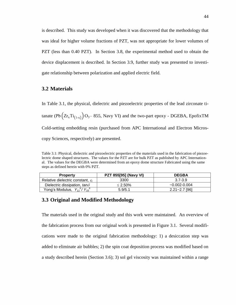
44
is described. This study was developed when it was discovered that the methodology that
was ideal for higher volume fractions of PZT, was not appropriate for lower volumes of
PZT (less than 0.40 PZT). In Section 3.8, the experimental method used to obtain the
device displacement is described. In Section 3.9, further study was presented to investi-
gate relationship between polarization and applied electric field.
3.2 Materials
In Table 3.1, the physical, dielectric and piezoelectric properties of the lead zirconate ti-
tanate (Pb (ZrxTi(1-x)) O3– 855, Navy VI) and the two-part epoxy - DGEBA, EpofixTM
Cold-setting embedding resin (purchased from APC International and Electron Micros-
copy Sciences, respectively) are presented.
Table 3.1: Physical, dielectric and piezoelectric properties of the materials used in the fabrication of piezoe-
lectric dome shaped structures. The values for the PZT are for bulk PZT as published by APC Internation-
al. The values for the DEGBA were determined from an epoxy dome structure Fabricated using the same
steps as defined herein with 0% PZT.
Property PZT 855[95] (Navy VI) DEGBA
Relative dielectric constant, r 3300 3.7-3.9
Dielectric dissipation, tan 2.50% ~0.002-0.004
Yong’s Modulus, Y11E/ Y33
E 5.9/5.1 2.21~2.7 [96]
3.3 Original and Modified Methodology
The materials used in the original study and this work were maintained. An overview of
the fabrication process from our original work is presented in Figure 3.1. Several modifi-
cations were made to the original fabrication methodology: 1) a desiccation step was
added to eliminate air bubbles; 2) the spin coat deposition process was modified based on
a study described herein (Section 3.6); 3) sol gel viscosity was maintained within a range

45
of 150-200mPas; and 4) Corona poling was used instead of the Contact Parallel Plate Pol-
ing.
An overview of the fabrication methodology used for this work is provided in
Figure 3.2. The volume fraction of PZT was varied from 0.0 to 0.7. First, the PZT pow-
der (purchased from APC International) was ball milled for 24 hours, where the mean
diameter of the PZT after the ball mill step was observed to be 0.97 microns. Next, ade-
quate amounts of the PZT and the epoxy were weighed and mixed with ethanol (15ml) by
hand. The subsequent mixture was then subjected to sonication for 2 hours, desiccated
for 4 hours, and then subjected to sonication for an additional hour. In this process, the
sonication and desiccation steps were used to distribute the PZT particles within the ma-
trix, enhance the evaporation of the ethanol and reduce the presence of air bubbles. The
dynamic viscosity of the mixture was then measured using a Brookfield DV-E viscosity
meter. Samples that had initial viscosity values less than 150mPas were subjected to ad-
ditional sonication until the final viscosity was within the range of 150 to 200 mPas
@100rpm. The resulting mixture was spin coated (using Speed/Time Profile 3 in Figure
3.5) onto a dome shaped Type 304, stainless steel substrate (purchased from Alfa Aesar,
Ward Hill, MA, USA). The dimensions for the dome structure are provided in Figure
3.3. Once deposited, the dome shaped composite thick films were cured over a hot plate
at 75° C for 8 h. A minimum of three samples were prepared for each volume fraction of
PZT (PZT volume fraction was varied from 0.0 –0.70). These measurements were aver-
aged to obtain the nominal thickness for each film. The dome shaped stainless steel sub-
strate was made by pressing the stainless steel substrate into a mold at a pressure of 500
psi for 15 minutes at room temperature.

46
Figure 3.1: Overview of the original method used from our previous work. Appropriate amounts of PZT,
DEGBA and ethanol were measured and mixed with the aid of a sonicator for 1 hour in the presence of air.
The DEGBA binder was then added and the subsequent mixture was sonicated for an additional 30
minutes. The final mixture was spin-coated onto dome shaped substrate and cured at 75C. Samples were
subsequently Parallel-Plate Contact poled at~2.2kV/mm [31].

47
Figure 3.2: Overview of the method of fabrication used for this work. The appropriate amounts of PZT,
DEGBA and ethanol were weighed and then mixed via a sonicator for 2 hours in the presence of air. The
mixture was subsequently dessicated for 4 hours to eliminate air bubbles. The mixture was sonicated
additional time. The binder was then added to the mixture and sonicated again, for an additional 30 mins.
The final mixture is spined coated onto dome-shaped stainless steel substrate, and cured at 75C. Samples
were poled via corona discharge.
Figure 3.3: The dimensions for the dome shape mold.

48
The piezoelectric dome structures were heated using a hot plate for 10 minutes at
75 ° C prior to application of the poling electric field. A Corona polarization approach
was used to align the dipoles of the PZT phase along the thickness of the samples, using a
SL Rack Mount Power supply from Spellman Inc. One set of samples (that were com-
prised of 10%-70% volume fraction of PZT) was poled at 45kV/mm at a temperature of
75° C in air for 30 minutes. Another set of samples (samples comprised of 0.10, 0.20 and
0.30 volume fractions of PZT) were poled at 70kV/mm at 75° C for 30 minutes. The
former set of samples could be poled at a higher poling voltage due to the smaller amount
of PZT, while the others could not be poled at the higher voltage. No top electrodes were
used during the poling process. The samples were wrapped in aluminum foil to remove
residual charges for 24 hours after the poling process. The film thickness was measured
at 5 locations on the dome structure in positions that are illustrated in Figure 3.4. The
final thickness was the average of the 5 measurements.
Figure 3.4: The thickness measurement was taken at five different places, and averaged.
3.4 Piezoelectric and Dielectric Characterization
The piezoelectric strain coefficients, d33 and d31 were measured at the frequency of
110Hz using the PiezoMeter PM300. Frequency dependent capacitance, dielectric loss,
resistance, conductance, impedance and phase spectra were measured with an impedance
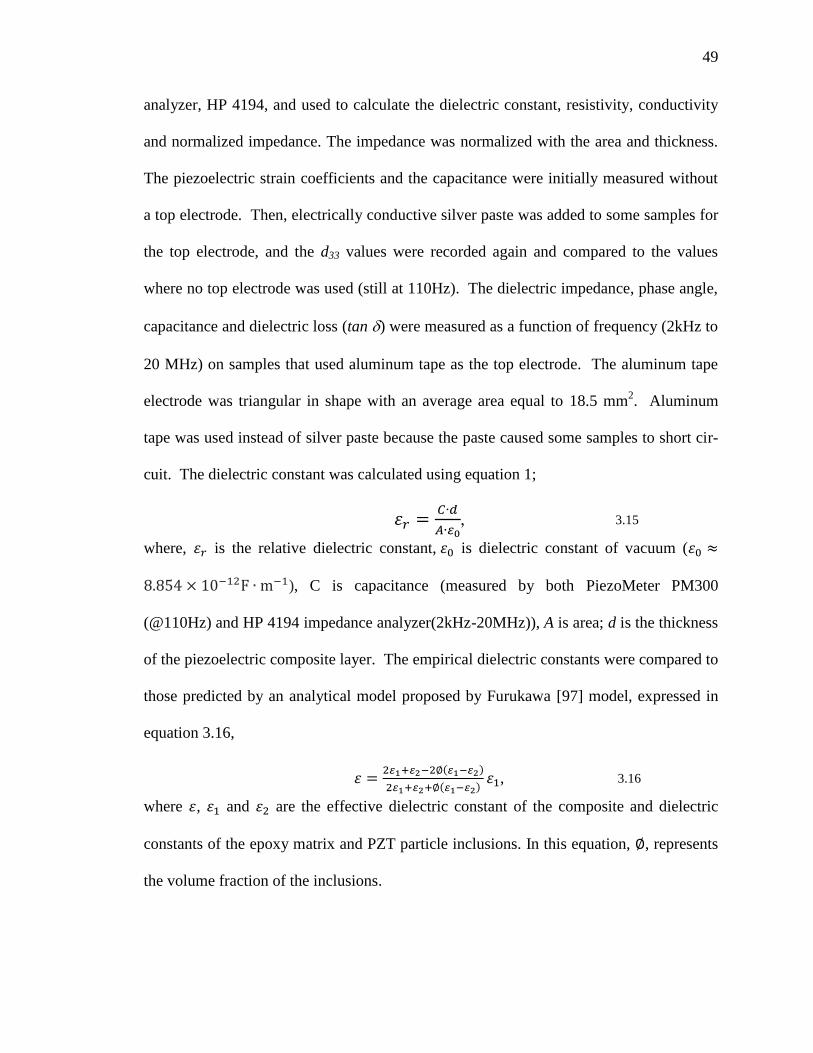
49
analyzer, HP 4194, and used to calculate the dielectric constant, resistivity, conductivity
and normalized impedance. The impedance was normalized with the area and thickness.
The piezoelectric strain coefficients and the capacitance were initially measured without
a top electrode. Then, electrically conductive silver paste was added to some samples for
the top electrode, and the d33 values were recorded again and compared to the values
where no top electrode was used (still at 110Hz). The dielectric impedance, phase angle,
capacitance and dielectric loss (tan ) were measured as a function of frequency (2kHz to
20 MHz) on samples that used aluminum tape as the top electrode. The aluminum tape
electrode was triangular in shape with an average area equal to 18.5 mm2. Aluminum
tape was used instead of silver paste because the paste caused some samples to short cir-
cuit. The dielectric constant was calculated using equation 1;
휀𝑟 =𝐶∙𝑑
𝐴∙𝜀0, 3.15
where, 휀𝑟 is the relative dielectric constant, 휀0 is dielectric constant of vacuum (휀0 ≈
8.854 × 10⁻¹²F ∙ m−1), C is capacitance (measured by both PiezoMeter PM300
(@110Hz) and HP 4194 impedance analyzer(2kHz-20MHz)), A is area; d is the thickness
of the piezoelectric composite layer. The empirical dielectric constants were compared to
those predicted by an analytical model proposed by Furukawa [97] model, expressed in
equation 3.16,
휀 =
2𝜀1+𝜀2−2∅(𝜀1−𝜀2)
2𝜀1+𝜀2+∅(𝜀1−𝜀2)휀1, 3.16
where 휀, 휀1 and 휀2 are the effective dielectric constant of the composite and dielectric
constants of the epoxy matrix and PZT particle inclusions. In this equation, ∅, represents
the volume fraction of the inclusions.

50
The measured piezoelectric strain coefficient, d33 was compared to the coefficients pre-
dicted by another model developed by Furukawa [18],
𝑑33 =
1
𝑐∙ ∅𝐿𝑠𝐿𝐸𝑑2𝑐2. 3.17
In equation 3.17, 𝑑33 is the piezoelectric coefficient; the subscripts 1 and 2, de-
note the matrix and PZT inclusions respectively. Also, in this equation,𝐿𝑠 =1
∅
𝑐1−𝑐
𝑐1−𝑐2 and
𝐿𝐸 =1
∅
𝜀1−𝜀
𝜀1−𝜀2 are parameters, where 𝑐, 𝑐1 and 𝑐2 are the Young’s Moduli of the compo-
site, matrix and PZT inclusions.
3.5 Characterization of Surface Morphology and Particle Distribution
The surface topology, morphology and distribution of the particles within the polymer
matrix were observed with the aid of scanning electron microscope (SEM) and Energy
Dispersive Spectroscopy (EDS) micrographs obtained from a Zeiss Sigma Field Emission
Microscope.
3.6 Spin-Speed/Time Profile Study
A spin coat speed and time increment study was performed to ascertain the ideal charac-
teristics for the spin coat and deposition step in the fabrication procedure. An overview
of the spin coat speed and time interval profiles examined are provided in Figure 3.5.
This study was done on samples that were comprised of 0.50 volume fraction of PZT,
where the viscosity of the sol gel was maintained at ~164.5 mPas @100 rpm. The
amount of sol gel and total spin coat time was maintained at 2 mL and 220 seconds, re-
spectively.
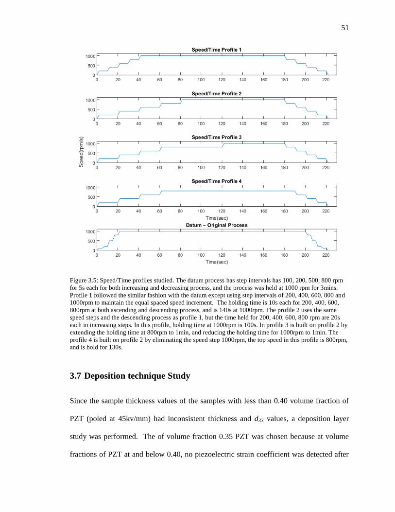
51
Figure 3.5: Speed/Time profiles studied. The datum process has step intervals has 100, 200, 500, 800 rpm
for 5s each for both increasing and decreasing process, and the process was held at 1000 rpm for 3mins.
Profile 1 followed the similar fashion with the datum except using step intervals of 200, 400, 600, 800 and
1000rpm to maintain the equal spaced speed increment. The holding time is 10s each for 200, 400, 600,
800rpm at both ascending and descending process, and is 140s at 1000rpm. The profile 2 uses the same
speed steps and the descending process as profile 1, but the time held for 200, 400, 600, 800 rpm are 20s
each in increasing steps. In this profile, holding time at 1000rpm is 100s. In profile 3 is built on profile 2 by
extending the holding time at 800rpm to 1min, and reducing the holding time for 1000rpm to 1min. The
profile 4 is built on profile 2 by eliminating the speed step 1000rpm, the top speed in this profile is 800rpm,
and is hold for 130s.
3.7 Deposition technique Study
Since the sample thickness values of the samples with less than 0.40 volume fraction of
PZT (poled at 45kv/mm) had inconsistent thickness and d33 values, a deposition layer
study was performed. The of volume fraction 0.35 PZT was chosen because at volume
fractions of PZT at and below 0.40, no piezoelectric strain coefficient was detected after

52
polarization at 45kV/mm when the sol viscosity was between 150 to 200 mPas. The in-
fluences of the number of deposition layers, time interval between layer deposition and
sol gel viscosity were examined in this study to understand how they influenced the final
thickness of the samples.
An overview of the deposition layer process studies is provided in Figure 3.6.
The steps before deposition were kept the same as those depicted in Figure 3.2. For each
sample fabricated, the amount of sol gel was maintained at 2ml. Sample were fabricated
at viscosities equal to 150, 248.7 and 299mPas (equipment operated at 100rpm).
The films were deposited in one, two or three layers as shown in Figure 3.6. The overall
amount of sol gel was maintained for each process and the same speed/interval profile
was maintained for each layer deposition step. The Datum sample included one deposi-
tion layer, where the measured viscosity prior to application of the single layer was
150mPas. Process A included two data sets, where the first set of samples was fabricated
with one deposition layer at a measured viscosity equal to 248.7mPas and the second data
set had a viscosity of 299mPas. Processes B, C and D incorporated two layers of deposi-
tion. Three sets of samples were prepared using Process B where the measured viscosities
for each data set were equal to 150, 248.7 and 299 mPas, respectively. The time interval
between the deposition of the first and second layers (for Process B) was three minutes.
Similarly, three sets of samples were prepared using Processes C and D, and the viscosi-
ties were measured to be equal to 150, 248.7 and 299 mPas, respectively. The time inter-
vals between the deposition of the first and seconds layers were 9 and 3 minutes for Pro-
cess C, and 18 and 5 minutes for Process D. Three layers of deposition were used for

53
Processes E and F, and three sets of samples were prepared at viscosity values equal to
150, 248.7 and 299 mPas, respectively.
The time increments between the deposition of the layers for Process E were equal to 29,
3 and 3 minutes, respectively, and equal to 44, 5 and 5 minutes, respectively for Process
F. Process G was implemented for the fabrication of two data sets of samples at viscosi-
ties equal to 248.7 and 299 mPas, respectively. A single time interval of 63 minutes was
taken prior to the deposition of the first and only layer.
The piezoelectric dome shaped composites underwent polarization following the process
described in Figure 3.2 after the layer(s) were deposited onto the stainless steel substrate
and pressed. The devices were Corona polarized at 45kV/mm, and were allowed to age
one day before the measurement of the piezoelectric strain coefficients, thicknesses and
dielectric properties.

54
Figure 3.6: Overview of the deposition layer and sol viscosity study. All of the processes described in this figure incorporated Speed/Interval Profile 3 for the
“Deposition” step. Three viscosity settings were used in this study: 150 mPas, 248.7 mPas and 299 mPas.

55

56
3.8 Device displacement
The displacement was a measured as a function of applied electrical voltage using a laser
interferometer (KeyenceLK-G10). An overview of the experimental set-up is provided in
Figure 3.7. The sample was placed on an insulated plate with the curved face (dome) fac-
ing down. The laser light from the interferometer was focused on the highest point on the
dome-shaped device. The electrical voltage was applied using a Corona charge set-up,
where the voltage was delivered from a needle connected with high voltage. The voltage
applied was linearly increased from 1kV/mm to 20kV/mm in increments of increases
0.2kV every 200 seconds.
Figure 3.7: Displacement testing set-up
The surface topology, morphology and distribution of the particles within the poly-
mer matrix were observed with the aid of scanning electron microscope (SEM) and Ener-
gy Dispersive Spectroscopy (EDS) micrographs obtained from a Zeiss Sigma Field Emis-
sion Miscroscope.

57
3.9 P-E hysteresis
The P-E hysteresis loop of (50%)PZT and (60%)PZT were measured by Precision Fer-
roelectric Tester from Radiant technology Inc.

58
Chapter 4
Results and Discussion
4.1 Chapter Organization
In this chapter, the results from our prior work[31], are compared to the results obtained
from a parametric study of processing parameters. In section 4.2, electrical properties of
epoxy single phase are presented. In Section 4.3 the results from optimized processing
procedure are presented and compared to the results from our prior work[31]. In order to
achieve the optimized processing steps described in Chapter 3, Section 4.4, a parametric
study was performed to identify the influence of spin-speed/time profiles on the resulting
piezoelectric and dielectric properties of the dome-shaped devices. In Sections 4.5, a
study on deposition technique was performed to investigate the influence of several pa-
rameters in deposition on 0.1-0.35 volume fraction of PZT. In section 4.6, the optimized
processing conditions are summarized. In section 4.7 and 4.8, the device displacements
and hysteresis were measured on selected composites.
4.2 Epoxy Dome Device
The epoxy single-phase dome-shaped samples were fabricated with exactly same proce-
dure with other samples (0.1-0.7 PZT), so that the composite samples could be to this
base study.

59
0 10000000 20000000
3.6
3.7
3.8
3.9
Average dielectric constant of Epoxy single phase
Average Loss of Epoxy single phase
Frequency (Hz)
Ave
rage d
iele
ctric
const
ant
-0.004
-0.002
0.000
0.002
0.004
0.006
Ave
rage L
oss
Figure 4.1: Dielectric constant/loss vs frequency of epoxy single phase samples, the spectrum was meas-
ured with small aluminum tape.
In Figure 4.1, the loss of epoxy single phase is mostly between 0.002-0.004, the
negative values could be equipment’s error. .
0 10000000 20000000
-0.000005
0.000000
0.000005
0.000010
Ave
rag
e c
ond
uctivity (
S/m
)
Frequency (Hz)
Average conductivity
Figure 4.2: Conductivity vs frequency of epoxy single phase samples, the spectrum was measured with
small aluminum tape.

60
0 10000000 20000000
0
200
400
Avera
ge R
esis
tivity (
ohm
/m)
Frequency (Hz)
Average Resistivity
Figure 4.3: Resistance vs frequency of epoxy single phase samples, the spectrum was measured with small
aluminum tape.
0 10000000 20000000
0
50000
100000
150000
Average Impedance of Epoxy single phase
Average Phase of Epoxy single phase
Frequency (Hz)
Ave
rag
e I
mp
ed
an
ce (
oh
m)
-90.2
-90.0
-89.8
-89.6
Ave
rag
e P
ha
se
Figure 4.4: Impedance/Phase vs frequency of epoxy single phase samples, the spectrum was measured with
small aluminum tape.

61
4.3 PZT-Epoxy Dome Results for Optimized Fabrication Method
To address the issues such as air bubbles and agglomerations of PZT, the sonication time
was increased in order to achieve better dispersion of PZT particles within the sol gel pri-
or to deposition of the layer. Also a desiccation step is also added to reduce the air
trapped in the sol. PZT volume fractions that ranged from 0.10 to 0.70 were fabricated,
and polarized Corona charges at 45kv/mm. All the viscosities prior to deposition were
maintained in 150mpas~200mPas range. The viscosity values are shown in Table 4.1.
(To meet the viscosity requirement, sols of lower volume fractions required longer curing
times ~2-3hours longer during the last sonication step), all sample are fabricated with
spin-speed/time profile 3.
Table 4.1 Measurement of viscosity
As in all four volume fractions presented in Table 4.1, the viscosities were within
range 150mPas-200mPas, but the thickness were not similar. Especially for 0.5 volume
fraction of PZT, the viscosity is similar to the viscosity of 0.7 volume fraction of PZT,
but the thickness is 39m lower when compared to 0.7 volume fraction of PZT.
Volume fraction of PZT
Average thickness (Microns) Viscosity (mPas @100rpm)
0.7 0.178 158.4
0.6 0.188 175.5
0.5 0.139 159.5
0.4 0.136 194.7

62
0.0 0.2 0.4 0.6 0.8
0
5
10
15
d33 values presented this work (no electrodes)
Predicted values by Furukawa's Model
d33 values from previous work
d33 values presented in this work(with silver paste as top electrode)
Pie
zoele
ctr
ic c
oeffic
ient d33 (
pC
/N)
Volume fractions of PZT
Figure 4.5: Piezoelectric longitudinal coefficient d33 values of this work (without top electrode), this work
(with silver paste as top electrodes), previous work, and predicted values by Furukawa are plotted. The d33
values presented in this work, have been
The longitudinal piezoelectric coefficient d33 values obtained by this work with
and without electrodes, the previous d33 values and d33 values predicted by Furukawa’s
analytical model[97] are shown in Figure 4.5. When tested without top electrodes, d33
values from this work and previous work both are increasing with the volume fractions of
PZT, similar trend has been found in other PZT-polymer composite[97, 98]. B Satish et
al[99] fabricated PZT-PVDF 0-3 composites; the piezoelectric coefficient d33 they report-
ed also shown a positive correlation with the increasing volume fractions of PZT, the
highest d33 they reported was 25pC/N, from 0.7 volume fraction of PZT. It is comparable
with our present results which is 11.106 pC/N @70% PZT as they use PVDF, which also
has piezoelectric coefficient d33 around 28 pC/N[99], as the matrix.
63
d33 values obtained by this work is one magnitude higher than values obtained from pre-
vious work. This could because (1) we increased the sonication time, which will result in
better dispersion of PZT particles. (2) The corona poling allowed us to pole the samples
at a higher voltage, which will improve the efficacy of the polarization process.
The experimental values obtained in present work are in agreement with theoreti-
cal values; in higher volume fractions of PZT the experimental values are even higher
than predicted values. Also a sharp drop in d33 at 0.3 volume fraction of PZT could be
observed in our present work. The d33 measured with silver paste as top electrode is simi-
lar or smaller than original measurement (i.e. measurement captured on same samples but
no electrodes were applied), this could because during the process of applying the silver
paste on top of the film, some silver paste found its way through the film and eventually
connected to the bottom stainless steel substrate causing the sample to short cuircuit.
The transvers piezoelectric coefficients -d31 values of this work and previous
work are shown in Figure 4.6, the values of our present work are also comparable to oth-
ers, 4pC/N @(0.21) PZT-PVDF 0-3 composites fabricated by Furukawa et al[100].

64
0.0 0.2 0.4 0.6 0.8
0
1
2
3
4
5
Tra
nsvers
e p
iezoele
ctr
ic c
oeffic
ient -d
31 (
pC
/N)
Vol. fractions of PZT
-d31 values from this work (no electrode)
-d31 values from our previous work
Figure 4.6: Piezoelectric coefficient -d31 values of this work and previous work. The samples from previ-
ous work were contact poled, and the samples from this work were corona charges poled at 45kv/mm.
There was no electrode applied in both cases.
0.0 0.2 0.4 0.6 0.8
5
10
15
20
25
30
35
40
45
50
55
60
65
70
75
80
85
90
Dielectric constant presented in this work
Predicted dielectric constant by Furukawa
Dielectric constant from previous work
Die
lectr
ic c
on
sta
nt
pre
se
nte
d in
th
is w
ork
Volume frctions of PZT
Figure 4.7: Dielectric constant of present work, previous work and predicted values by Furukawa. No elec-
trodes applied in both cases.

65
Dielectric constant is tested under the room condition @110Hz. In both previous
work and this work, the dielectric constants are increasing with the volume fractions of
PZT. The dielectric constant of this work is smaller than previous work, this could be-
cause of the reduction of the agglomeration of PZT. As in Figure 4.7, the experimental
values and the predicted values have similar trends, and experimental values and predict-
ed values are comparable.
Comparison in important properties between previous work and this present work
at 0.7 volume fraction of PZT are shown in Table 4.2 Comparison between corona poled
and contact poled data in 70% PZTTable 4.2
Table 4.2 Comparison between corona poled and contact poled data in 70% PZT
Contact poled 0.7 PZT Corona poled 0.7 PZT
Piezoelectric strain coefficient, d33 1.18pC/N 11.11pC/N
Piezoelectric strain coefficient, d31 0.75pC/N 3.73pC/N
Dielectric constant 76.10048 53.87

66
0.1 0.2 0.3
0.0
0.2
0.4
0.6
0.8
1.0
1.2
1.4
1.6
1.8
2.0
2.2
2.4
2.6
2.8
Longitudin
al pie
zoele
ctr
ic s
tain
coeffic
ient d33 (
pC
/N)
Volume fractions of PZT
d33 (Poled at 45kv/mm) in this work
Average d33 (Poled at 70kv/mm)
d33 values from previous work
d33 values predicted by Furukawa
0.1 0.2 0.3
0.2
0.4
0.6
0.8
1.0
1.2
1.4
1.6
1.8
2.0
2.2
2.4
2.6
2.8
3.0
3.2
3.4
Tra
nsvers
e p
iezoele
ctr
ic c
oeffic
ient -d
31 (
pC
/N)
Volume fractions of PZT
-d31 from this work(Poled at 45kv/mm)
-d31 from this work (Poled at 70kv/mm)
-d31 values from our previous work
Figure 4.8: Longitudinal piezoelectric coefficient d33 and transverse piezoelectric coefficient d31 of previous
work, this work (corona poled at 70kv/mm), this work (corona poled at 45kv/mm) and predicted values
from Furukawa(only for d33).
From Figure 4.8, the d33 values of samples poled under 70kv/mm are substantially
higher than samples poled with 45kv/mm, with same volume fractions of PZT. The pie-

67
zoelectric coefficient d33 captured from samples poled at 70kv/mm are more in agreement
with the predicated values than samples poled with 45kv/mm. But d31 values are similar
in both sets of samples, both sets of corona poled samples have higher - d31 values than
previous work.
Frequency spectrums of properties of samples fabricated by updated methods are
shown below.

68
0 10000 20000
15
20
25
30
35
40
45
Ave
rag
e d
iele
ctr
ic c
onsta
nt
of
pre
vio
us w
ork
Frequency (kHz)
Dielectric constant of PZT(0.1)
Dielectric constant of PZT(0.2)
Dielectric constant of PZT(0.3)
Dielectric constant of PZT(0.4)
Dielectric constant of PZT(0.5)
Dielectric constant of PZT(0.7)
0 10000 20000
14
16
18
20
22
24
26
28
30
32
34
36
38
40
42
44
46
Dielectric constant of PZT(0.1)
Dielectric constant of PZT(0.2)
Dielectric constant of PZT(0.3)
Dielectric constant of PZT(0.4)
Dielectric constant of PZT(0.5)
Dielectric constant of PZT(0.6)
Dielectric constant of PZT(0.7)
Die
lectr
ic c
onsta
nt of pre
sent w
ork
Frequency (kHz)
Figure 4.9: The dielectric spectroscopy (2kHz-20MHz) of previous work and this work, the spectrums were
obtained with small triangular aluminum tape as top electrode in both cases.
The capacitance was measured, and then the dielectric constant was calculated for
both previous work and present work. As our frequency range is 2kHz-20MHz, space
charge polarization that mostly responsible for lower frequencies could not be clearly ob-

69
served in Figure 4.9 (this is because due to the equipment, the second measurement fre-
quency is 50kHz). Within 2kHz~1MHz, the spectrums show mostly dipolar polarizations
and since space charge polarizations could not follow the frequencies, the dielectric con-
stant shows a decreasing trend versus the increasing frequency. Within 1MHz~10MHz,
the frequency dependence of the dielectric constant is very low and this polarization is
mostly the result of ionic mechanism. The increasing dielectric constant with frequency
above 10MHz could be resulted from the epoxy phase, since in Figure 4.1, epoxy single
phase samples show a substantial positive correlation with the increasing frequency.
In corona poled samples and contact poled samples’ spectrums, dielectric con-
stants are increasing with the volume fractions of PZT. The dielectric constant of present
work is smaller than previous work; this could because the reduction of the sample thick-
ness, as there was less dielectric material. The dielectric constants are less dependent on
frequencies too.

70
0 10000 20000
0.00
0.01
0.02
0.03
0.04
0.05
0.06
0.07
0.08
0.09
Dis
sip
ation
fa
cto
r of
pre
vio
us w
ork
Frequency (kHz)
Loss of PZT(0.1)
Loss of PZT(0.2)
Loss of PZT(0.3)
Loss of PZT(0.4)
Loss of PZT(0.5)
Loss of PZT(0.7)
0 10000 20000
0.000
0.005
0.010
0.015
0.020
0.025
0.030
0.035
0.040
Loss of PZT(0.1)
Loss of PZT(0.2)
Loss of PZT(0.3)
Loss of PZT(0.4)
Loss of PZT(0.5)
Loss of PZT(0.6)
Loss of PZT(0.7)
Dis
sip
ation facto
r of pre
sent w
ork
Frequency (kHz)
Figure 4.10: Dissipation factor verse frequency (2kHz-20MHz) of previous work and this work, the spec-
trums were obtained with small triangular aluminum tape as top electrode for both cases.
Figure 4.10 shows the dissipation factors of both contact poled corona poled sam-
ples; in both cases the dissipation factors increase with the volume fractions of PZT. The
dissipation factor of PZT (~2.5%) is relatively higher than epoxy matrix (0.002~0.004).

71
The spectrums also show a substantial increase with the frequency, as epoxy’s dissipation
factor is relatively stable, this increase is largely due to PZT inclusions. The dissipation
factors of present work are smaller than previous work as the samples fabricated by up-
dated methods this could because the reduction of air trapped in samples and better dis-
tribution of PZT in the epoxy matrix.
0 10000 20000
0
5000
10000
15000
20000
25000
30000
Norm
aliz
ed Im
pedance
Frequency (kHz)
Normalized impedance of PZT (0.1)
Normalized impedance of PZT (0.2)
Normalized impedance of PZT (0.3)
Normalized impedance of PZT (0.4)
Normalized impedance of PZT (0.5)
Normalized impedance of PZT (0.7)
0 10000 20000
0
10000
20000
30000 Average normalized Impedance of PZT(0.1)
Average normalized Impedance of PZT(0.2)
Average normalized Impedance of PZT(0.3)
Average normalized Impedance of PZT(0.4)
Average normalized Impedance of PZT(0.5)
Average normalized Impedance of PZT(0.6)
Norm
aliz
ed im
pedance o
f pre
sent w
ork
(ohm
*m)
Frequency (kHz)

72
Figure 4.11: Normalized impedance verse frequency (2kHz-20MHz) of previous work and this work, the
spectrums were obtained with small triangular aluminum tape as top electrode for both cases.
Shown in Figure 4.11, the impedance in both previous work and present work de-
crease with the volume fractions of PZT. Compared to previous work, the impedances are
higher in present work.
0 10000 20000
-90
-89
-88
-87
Ph
ase o
f p
revio
us w
ork
Frequency (kHz)
Phase of PZT(0.1)
Phase of PZT(0.2)
Phase of PZT(0.3)
Phase of PZT(0.4)
Phase of PZT(0.5)
Phase of PZT(0.6)
0 10000 20000
-90.0
-89.8
-89.6
-89.4
-89.2
-89.0
-88.8
-88.6
-88.4
-88.2
-88.0
-87.8
-87.6
-87.4
-87.2
-87.0 Average phase of PZT (0.1)
Average phase of PZT (0.2)
Average phase of PZT (0.3)
Average phase of PZT (0.4)
Average phase of PZT (0.5)
Average phase of PZT (0.6)
Average phase of PZT (0.7)
Phase for
pre
sent w
ork
Frequency (kHz)

73
Figure 4.12: Phase verse frequency (2kHz-20MHz) of previous work and this work, the spectrums were
obtained with small triangular aluminum tape as top electrode for both cases.
In a pure capacitive circuit, the phase of voltage will be 90 behind the alternative
current. As seen in Figure 4.12 in both previous and present work, the phases increase
with frequency, as the materials will be less dielectric in high frequency region. Phase
increases are also increase with volume fractions of PZT. Phases in each volume fractions
in present work are lower than the corresponding part in previous work, this could indi-
cate that the updated method has better capacitive property.

74
0 10000 20000
-5
0
5
10
15
20
25
30
35
40
45
50
55
60
65
70
75
80
85
Resis
tivity o
f pre
vio
us w
ork
(ohm
/m)
Frequency (kHz)
Resistivity(0.1)
Resistivity(0.2)
Resistivity(0.3)
Resistivity(0.4)
Resistivity(0.5)
Resistivity(0.7)
0 10000 20000
-5
0
5
10
15
20
25
30
35
40
45
50
55
60
65
70
75
80
85
Resis
tivity o
f pre
sent w
ork
(ohm
/m)
Frequency (kHz)
Average resistivity of PZT(0.1)
Average resistivity of PZT(0.2)
Average resistivity of PZT(0.3)
Average resistivity of PZT(0.4)
Average resistivity of PZT(0.5)
Average resistivity of PZT(0.6)
Average resistivity of PZT(0.7)
Figure 4.13: Resistivity verse frequency (2kHz-20MHz), these samples are fabricated with updated meth-
od; the spectrums were obtained with small triangular aluminum tape as top electrode.
Similar to impedance spectrum, Figure 4.11 shows that resistivity decreases with
the increasing PZT volume fractions. And the resistivity of previous work is lower than

75
present work, together with impedance spectrum, could indicated that the samples fabri-
cated with updated method could have lower leakage current.
0 10000 20000
-0.0001
0.0000
0.0001
0.0002
0.0003
0.0004
0.0005
0.0006
0.0007
0.0008 Average Conductivity of PZT(0.1)
Average Conductivity of PZT(0.2)
Average Conductivity of PZT(0.3)
Average Conductivity of PZT(0.4)
Average Conductivity of PZT(0.5)
Average Conductivity of PZT(0.6)
Average Conductivity of PZT(0.7)
Conductivity
Frequency (kHz)
Figure 4.14: Conductivity verse frequency (2kHz-20MHz), these samples are fabricated with updated
method; the spectrums were obtained with small triangular aluminum tape as top electrode.
The conductivity of the present work is found to be increasing with the increase of
volume fractions of PZT and the frequency, similar as A. Seema et al[98].
Figure 4.15: Surface of PZT (0.5)-Epoxy 0-3 dome shape structure.

76
Figure 4.16: Surface of PZT (0.6)-Epoxy 0-3 dome shape structure.
Figure 4.15 and Figure 4.16 shows the surface morphology of 50%PZT and
60%PZT composites. PZT particles haven been using in the study has mean diameters as
0.97μm, has comparable size to the clusters shown in Figure 4.15 and Figure 4.16, this
indicated that PZT particles are well distributed in epoxy matrix, no significant agglom-
erations are observed. There were no pores observed in both SEM images.
Figure 4.17: EDS images of PZT(0.5)-Epoxy 0-3 dome shape structure. A) SEM images with distribution
of Pt, Zr and Ti. B) Distribution of Pb. C) Distribution of Zr. D distribution of Ti.

77
Figure 4.18: EDS images of PZT (0.6)-Epoxy 0-3 dome shape structure. A) SEM images with distribution
of Pt, Zr and Ti. B) Distribution of Pb. C) Distribution of Zr. D distribution of Ti.
Figure 4.17 and Figure 4.18 shows EDS images of 50%PZT and 60%PZT compo-
sites, further indicate the distribution of PZT in epoxy matrix.
4.4 Spin-speed/time profile study
Originally we used the spin coat speed and time intervals describe in the previous paper,
however since a few changes are made in fabrication methods (Fixed the ethanol usage in
this study, increase the amount of time in the original sonication and adding desiccation
and sonication steps) the sample fabricated could not present electromechanical respons-
es. The spin coat speed and time intervals are designed by experiments described in Table
4.3. All steps before spin coating are maintained as main procedure. And in the spin coat-
ing process, 4 combinations of spin coating speeds and time intervals are studied. This
study was done on 50% of PZT in volume fractions, the viscosity prior to deposition is
164.5mPas @100rpm.

78
We studied how the spin-coating time intervals and speed will affect the thickness of the
sample, and eventually affect the piezoelectric and dielectric properties. This study was
performed at 50%PZT.
Table 4.3 Spin-speed/time profile study
As we could see from Table 4.3 the first sample which was fabricated with profile 1
shown no piezoelectric response.
Samples fabricated through profile 2 and 3 presents reasonable d33 value, but the cen-
ter of the sample fabricated through profile 2 appears to be thicker than elsewhere. Sam-
ples fabricated through profile 3 have uniform thickness throughout the whole sample,
and presents reasonable piezoelectric response.
4.5 Deposion technique study
The deposing techniques study was done on 0.35 PZT, this volume fraction of PZT was
chosen because of discontinuity in piezoelectric property at volume fractions of PZT be-
low 0.4. There were 3 starting viscosities, 150mPas, 248.7mPas and 299mPas respective-
Average pie-zoelectric
layer thick-ness (mm)
Planned Poling voltage
(kv)
Planned Poling elec-
tric field (kv/mm)
d33(pC/N) Capaci-tance (pF)
Calculated die-lectric constant
comment
Profile (1)
0.105 4.7 45 -0.04 10.5 25.36
The d33 values here shown is within the mar-
gin of the equipment
Profile (2)
0.141 6.3 45 7.26 13.9 45.08 Higher at center where is thicker
Profile (3)
0.177 8 45 7.52 15 61.07
Profile (4)
0.241 10.8/7.8 45 4.27 18.3 101.44 Short circuit @45kv/mm
Datum 0.089 4.1 45 0.02 9.8 20.06

79
ly, chosen from 150-200mPas, 200-250mPas, and 250-300mPas ranges to investigate the
influence of viscosity on piezoelectric and dielectric properties.
There were 8 processes including our datum study are employed, this allows us to inves-
tigate the influence of time between depositions and the numbers of layer on piezoelectric
and dielectric properties.
Table 4.4 Deposition techniques study's results
Profile Viscosity
tested d33
Average capacitance
(pF)
Piezoelectric layer thick-ness (mm)
Calculated dielectric constant
Corona poling electric
field
Datum study
150mPas -0.02 22.9 0.065 34.23953 45kv/mm
Process A
248.7mPas 0.01 21.7 0.087 43.42681 45kv/mm
299.3mPas 0.02 22.4 0.115 59.25498 45kv/mm
Process B
150mPas 0.02 20.8 0.085 40.66879 45kv/mm
248.7mPas 0.02 20.8 0.127 60.76396 45kv/mm
299.3mPas 4.32 20.08 0.147 67.89848 45kv/mm
Process C
150mPas 0.02 23.22 0.093 49.67343 45kv/mm
248.7mPas 0.01 22.3 0.113 57.96453 45kv/mm
299.3mPas 5.45 20.94 0.149 71.76983 45kv/mm
Process D
150mPas 0.03 24 0.103 56.8627 45kv/mm
248.7mPas 5.78 19.9 0.141 64.5433 45kv/mm
299.3mPas 5.51 19.25 0.167 73.94796 45kv/mm
Process E
150mPas 5.51 20.5 0.129 60.83066 45kv/mm
248.7mPas 5.74 18.43 0.173 73.35487 45kv/mm
299.3mPas 5.37 18.42 0.179 75.84407 45kv/mm
Process F
248.7mPas 4.62 15.4 0.217 76.87045 Dielectric
break down @45kv/mm
299.3mPas 4.02 15.76 0.227 82.29265 Dielectric
break down @45kv/mm
Process G
248.7mPas 0.04 19.45 0.118 52.79352 45kv/mm
299.3mPas 4.34 19 0.143 62.49836 45kv/mm
As we can see in the table, the sample fabricated with our datum process shown
no piezoelectric response, neither do samples fabricated through process A, which have
elevated viscosities.

80
Process B, C and D are involved with two times deposition. Samples with all vis-
cosity fabricated through process B experience no piezoelectricity. Sample has viscosity
as 299mPas, fabricated through process C, shows longitudinal piezoelectric coefficient
after poled by 45kv/mm, the value captured here is comparable to 0.4 volume fraction of
PZT sample, which is 5.6pC/N respectively. Samples fabricated though the same process
but with lower viscosity still shown no piezoelectric response. Fabricated though process
D, samples fabricated with higher viscosity (i.e. 248.7mPas and 299mPas) experience
piezoelectricity.
Process E and F are involved with three times deposition. Fabricated through E,
samples with all viscosities tested shown reasonable longitudinal piezoelectric coeffi-
cient. Only two samples were fabricated through process F, and both them experienced
dielectric break down during the poling process, there d33 values are lower compared to
other sample with same volume fraction.
And when the starting viscosity is high enough, and waited for a longer time, 1h, respec-
tively, the samples fabricated through Process G, similar to datum process could also
have piezoelectric charge coefficients measurement, as the container was covered during
the whole experiment period which avoided the evaporation of ethanol, this could come
from the viscosity increase by the epoxy hardener.
All these studies show that, within the range of viscosity we decided for higher
PZT volume fractions (0.4~0.7), lower volume fractions of PZT (0.1~0.3) requires multi-
ple depositions to achieve the favorable thickness. And with the increasing viscosity and
right technique, the samples of lower volume fractions of PZT (0.1~0.3) could also be
possible to fabricate with single deposition. If the thickness is to maintain, we should ei-

81
ther increase the viscosity reading to 300mPas-350mPas or fabricate through profile 5
when the viscosity is maintained in 150-200mPas.
4.6 Summary of the Optimized Processing Conditions
The spin/speed profile 3 offers most uniform surface, and reasonable longitudinal piezoe-
lectric d33 was observed, the d33 value is 7.52pC/N at 05 volume fraction of PZT. Com-
pared to contact poling, samples poled by corona charges experience stronger piezoelec-
tric effect. For volume fractions 0.4-0.7 of PZT, the original deposition method was suf-
ficient to achieve reasonable piezoelectric response, the values for d33 and -d31 were
11.11pC/N and -4pC/N respectively at 0.7 volume fraction of PZT. For volume fractions
0.1-0.35 of PZT, the process D (when the viscosity is within 200mPas-250mPas) should
be employed, the d33 value is 5.78pC/N at 0.35 volume fraction of PZT.
The agglomeration may be attributed to several mechanisms of agglomeration:
Brownian, gravitational, turbulent, and electrostatic, where the gravitational form is miti-
gated by the spin coating process. This can be validated through Figure 4.15 and Figure
4.16, where minimal coagulation of particles is observed at the interface of the substrate
and the composite. The as-received PZT powders tend to naturally form clusters that vary
between 5-20 µm in the case of aluminum and 10-25 µm in the case of PZT, where these
agglomerations are most likely attributed to electrostatic agglomeration. Addition of eth-
anol to the mixture did not effectively change the pH of the solution to negate the surface
charge on the all of the particles which most likely diminished its effectiveness in coun-
teracting the electrostatic forces between particles. The extent of the effectiveness of the

82
ethanol on the pH of the solution was also a function of the number of particles within the
colloidal sol gel.
4.7 Displacement measurement
Figure 4.19: Displacement data of 0.5 volume fraction of PZT .
Figure 4.19 shows the displacement of 0.5 volume fraction of PZT composites.
The displacement is increasing with the incremental voltage; the largest displacement is
3.7m, highest strain rate is 2.7%, found @20kV/mm.

83
Figure 4.20: Displacement data of 0.6 volume fraction of PZT.
Figure 4.20 shows the displacement of 0.6 volume fraction of PZT composites. The
displacement is also increasing with the incremental voltage; the largest displacement is
3.2m, highest strain rate is 1.7%, found @20kV/mm.
4.8 P-E Hysteresis loop.
The P-E hysteresis loos of 0.5volume fraction and 0.6 volume fraction are presented be-
low.

84
-100 -50 0 50 100
-0.05
0.00
0.05
0.10
0.15
Po
larizatio
n (
mic
ro C
/cm
^2)
C
750volt
Figure 4.21: Hysteresis loop of PZT(0.5)-Epoxy dome shape structure under 53.9kv/cm.(thickness
0.139mm)
-50 0 50
-0.1
0.0
0.1
0.2
Po
larizatio
n (
mic
ro C
/cm
^2)
Electric field (kv/cm)
1000vol
Figure 4.22: Hysteresis loop of PZT(0.6)-Epoxy dome shape structure under 58.48kv/cm.(thickness
0.188mm)

85
Chapter 5
Conclusions and Future work
5.1 Conclusions
Piezoelectric 0-3 composites PZT-Epoxy with PZT’s volume fractions 0%-70% are fab-
ricated using a combination of solvent and spin coat deposition technique. In the pre-
sented work, the fabrication methods are updated to improve longitudinal and transverse
piezoelectric coefficients in PZT-Epoxy 0-3 composites. Both longitudinal and transverse
piezoelectric coefficients are increasing with the volume fractions of PZT. Compared to
previous work, the piezoelectric characteristic is enhanced largely. This could because of
the employment of corona poling technique, and better mixing of the two phases. The
longitudinal piezoelectric coefficient d33 and dielectric constant are in agreement with
values predicted by Furukawa’s analytical model. Specifically, the values for d33, d31 and
dielectric constant were 11.11pC/N, -4pC/N and 56 respectively at 79% volume fraction
of PZT. Similar and lower values of the longitudinal piezoelectric coefficient d33 were
observed with silver paste as top electrode, this could because the silver pastes could cre-
ate electric pathway to cause samples to short circuit. Based on SEM images and EDS
micrographs obtained the agglomerations of PZT in the composite are largely reduced,
and the distribution of PZT in the composite are uniform. Dielectric constant is increasing
the volume fractions of PZT, this due to the increase in the effective dipole moment of
the piezoelectric component. The dielectric constant of the present work is smaller than

86
previous work in corresponding volume fractions, this could be a result of the reduction
of agglomeration of PZT. These results indicate that devices such as these may have po-
tential applications as energy harvester, actuator and capacitors. Corona poling with dif-
ferent voltages in lower volume fractions of PZT were studied additionally, the piezoe-
lectric response in longitudinal mode was improved; however there was no significant
improvement in transverse mode observed. There was clear dependence of impedance,
phase, dielectric constant, loss, conductivity and resistivity on the frequency. Like previ-
ous results, impedance, and phase are reducing with the increasing volume fractions of
PZT, and dielectric constant, conductivity and loss are increasing with the increasing vol-
ume fractions of PZT. The impedance and resistivity are increased compare to the corre-
sponding volume fractions in the previous work, this indicate less leakage current could
occur when subjected to alternative currents.
The spin-speed/time profiles were studied at 0.5 volume fractions of PZT ,sample fabri-
cated through profile 3 had largest piezoelectric coefficient d33 value, 7.52pC/N respec-
tively.
The discontinuity in longitudinal piezoelectric coefficient d33 was observed in
lower volume fractions of PZT (i.e. 0.1-0.3). To address the issue, a depositing technique
study at 0.35 volume fraction of PZT was carried out. The results shown that samples
fabricated with Process D (viscosity~200mPas~250mPad) had most optimized d33 value,
5.78pC/N respectively.
The displacement of 50% and 60% volume fraction of PZT were studied, the de-
vices were subjected to step increasing electric file. The largest electric field applied as
20kv/mm, half of the poling electric filed. The largest displacement of 50% and 60% vol-

87
ume fraction of PZT were observed as 3.7m and 3.2m, and the strain rate correspond-
ing were 2.7% and 1.7% respectively.
Lastly, the P-E hysteresis loops of 50% and 60% volume fraction of PZT are presented.
5.2 Future work
To further enhance the piezoelectric characteristics, the future work will include a con-
ductive third phase. The influence of the conductive third phase on piezoelectric behavior
will be further investigated by fabrication and analysis of three phase composites by vari-
ation of the PZT volume fraction and the volume fractions of the conductive third phase.
Dome shaped thick film composites will be fabricated to understand both the d33 and d31
piezoelectric strain characteristics. The dependence if impedance, dielectric constant, re-
sistivity and conductivity will be further studied. Devices displacement and P-E hystere-
sis will also be investigate.
88
References
[1] S. R. Anton and H. A. Sodano, "A review of power harvesting using piezoelectric
materials (2003–2006)," Smart materials and Structures, vol. 16, p. R1, 2007.
[2] J. Baker, S. Roundy, and P. Wright, "Alternative geometries for increasing power
density in vibration energy scavenging for wireless sensor networks," in Proc. 3rd
Int. Energy Conversion Engineering Conf.(San Francisco, CA, Aug.), 2005, pp.
959-70.
[3] S. Banerjee, "An experimental and theoretical analysis of two and three phase
epoxy based piezoelectric composites," Rutgers University-Graduate School-New
Brunswick, 2013.
[4] R. C. Buchanan, E. Park, R. Surana, H. Tennakone, and K. Tennakone, "High
piezoelectric actuation response in graded Nd2O3 and ZrO2 doped BaTiO3
structures," Journal of electroceramics, vol. 26, pp. 116-121, 2011.
[5] O. Delas, A. Berry, P. Masson, and Y. Pasco, "Optimizing the thickness of
piezoceramic actuators for bending vibration of planar structures," Journal of
Intelligent Material Systems and Structures, vol. 18, pp. 1191-1201, 2007.
[6] G. H. Haertling, "Ferroelectric ceramics: history and technology," J. Am. Ceram.
Soc., vol. 82, pp. 797-818, 1999.
[7] C.-H. Nguyen, S. Pietrzko, and R. Buetikofer, "The influence of temperature and
bonding thickness on the actuation of a cantilever beam by PZT patches," Smart
materials and structures, vol. 13, p. 851, 2004.
[8] A. Nisar, N. Afzulpurkar, B. Mahaisavariya, and A. Tuantranont, "MEMS-based
micropumps in drug delivery and biomedical applications," Sensors and
Actuators B: Chemical, vol. 130, pp. 917-942, 2008.
[9] L. APC International, Piezoelectric Ceramics: Principles and Applications: APC
International, 2002.
[10] D. Wang, Y. Fotinich, and G. P. Carman, "Influence of temperature on the
electromechanical and fatigue behavior of piezoelectric ceramics," Journal of
Applied Physics, vol. 83, pp. 5342-5350, 1998.
[11] S. Mall and T. Hsu, "Electromechanical fatigue behavior of graphite/epoxy
laminate embedded with piezoelectric actuator," Smart Materials and Structures,
vol. 9, p. 78, 2000.

89
[12] D. P. Wang and G. P. Carman, "Combined electrical and mechanical fatigue of
piezoelectric ceramics undergoing polarization switching for large displacement
actuation," 1998, pp. 210-221.
[13] J. E. Frank, G. H. Koopmann, W. Chen, and G. A. Lesieutre, "Design and
performance of a high-force piezoelectric inchworm motor," 1999, pp. 717-723.
[14] C. Caliendo, S. Sait, and F. Boubenider, "Love-Mode MEMS Devices for Sensing
Applications in Liquids," Micromachines, vol. 7, p. 15, 2016.
[15] A. Dogan, K. Uchino, and R. E. Newnham, "Composite piezoelectric transducer
with truncated conical endcaps" Cymbal"," Ultrasonics, Ferroelectrics, and
Frequency Control, IEEE Transactions on, vol. 44, pp. 597-605, 1997.
[16] S. Shahab, D. Tan, and A. Erturk, "Hydrodynamic thrust generation and power
consumption investigations for piezoelectric fins with different aspect ratios," in
ASME 2015 Conference on Smart Materials, Adaptive Structures and Intelligent
Systems, 2015, pp. V002T06A011-V002T06A011.
[17] H. Shen, F. S. Zhang, H. L. Ji, J. H. Qiu, and Y. X. Bian, "Self-powered semi-
passive vibration damping system based on self-sensing approach," in Seventh
International Symposium on Precision Mechanical Measurements. vol. 9903, L.
Yu, Ed., ed Bellingham: Spie-Int Soc Optical Engineering, 2016.
[18] Y. Jia, C. D. Do, X. D. Zou, and A. A. Seshia, "A Hybrid Vibration Powered
Microelectromechanical Strain Gauge," Ieee Sensors Journal, vol. 16, pp. 235-
241, Jan 2016.
[19] M. Kuna, "Fracture mechanics of piezoelectric materials – Where are we right
now?," Engineering Fracture Mechanics, vol. 77, pp. 309-326, 1// 2010.
[20] H. J. Hwang, M. Yasuoka, M. Sando, M. Toriyama, and K. Niihara, "Fabrication,
Sinterability, and Mechanical Properties of Lead Zirconate Titanate/Silver
Composites," Journal of the American Ceramic Society, vol. 82, pp. 2417-2422,
1999.
[21] S. Choi, H. Lee, and W. Moon, "A micro-machined piezoelectric hydrophone
with hydrostatically balanced air backing," Sensors and Actuators A: Physical,
vol. 158, pp. 60-71, 2010.
[22] H. Lee, S. Choi, and W. Moon, "A micro-machined piezoelectric flexural-mode
hydrophone with air backing: Benefit of air backing for enhancing sensitivitya),"
The Journal of the Acoustical Society of America, vol. 128, pp. 1033-1044, 2010.
[23] K. Cook-Chennault, N. Thambi, and A. Sastry, "Powering MEMS portable
devices—a review of non-regenerative and regenerative power supply systems

90
with special emphasis on piezoelectric energy harvesting systems," Smart
Materials and Structures, vol. 17, p. 043001, 2008.
[24] K. A. Cook-Chennault, N. Thambi, M. A. Bitetto, and E. Hameyie, "Piezoelectric
energy harvesting a green and clean alternative for sustained power production,"
Bulletin of Science, Technology & Society, vol. 28, pp. 496-509, 2008.
[25] H.-S. Yoon, G. Washington, and A. Danak, "Modeling, optimization, and design
of efficient initially curved piezoceramic unimorphs for energy harvesting
applications," Journal of Intelligent Material Systems and Structures, vol. 16, pp.
877-888, 2005.
[26] F. Amirouche, Y. Zhou, and T. Johnson, "Current micropump technologies and
their biomedical applications," Microsystem technologies, vol. 15, pp. 647-666,
2009.
[27] M. M. Teymoori and E. Abbaspour-Sani, "Design and simulation of a novel
electrostatic peristaltic micromachined pump for drug delivery applications,"
Sensors and Actuators A: Physical, vol. 117, pp. 222-229, 2005.
[28] J. P. Choi, K. S. Kim, Y. H. Seo, and B. H. Kim, "Design and fabrication of
synthetic air-jet micropump," International Journal of Precision Engineering and
Manufacturing, vol. 12, pp. 355-360, 2011.
[29] J. Harrison and Z. Ounaies, Piezoelectric polymers: Wiley Online Library, 2002.
[30] J. Dargahi, "Piezoelectric and pyroelectric transient signal analysis for detection
of the temperature of a contact object for robotic tactile sensing," Sensors and
Actuators A: Physical, vol. 71, pp. 89-97, 1998.
[31] S. Banerjee, W. Du, L. Wang, and K. Cook-Chennault, "Fabrication of dome-
shaped PZT-epoxy actuator using modified solvent and spin coating technique,"
Journal of Electroceramics, vol. 31, pp. 148-158, 2013.
[32] S. P. Marra, K. T. Ramesh, and A. S. Douglas, "The mechanical properties of
lead-titanate/polymer 0–3 composites," Composites Science and Technology, vol.
59, pp. 2163-2173, 11// 1999.
[33] S. N. Zhu, B. Jiang, and W. W. Cao, "Characterization of piezoelectric materials
using ultrasonic and resonant techniques," in Ultrasonic Transducer Engineering:
Medical Imaging 1998. vol. 3341, K. K. Shung, Ed., ed, 1998, pp. 154-162.
[34] K. M. Mossi, G. V. Selby, and R. G. Bryant, "Thin-layer composite unimorph
ferroelectric driver and sensor properties," Materials Letters, vol. 35, pp. 39-49,
1998.

91
[35] J. Peng, C. Chao, and H. Tang, "Piezoelectric micromachined ultrasonic
transducer based on dome-shaped piezoelectric single layer," Microsystem
technologies, vol. 16, pp. 1771-1775, 2010.
[36] Y. Man-Soon, H. Sung-Moo, and U. Soon-Chul, "A newly designed chopper for
pyroelectric infrared sensor by using a dome-shaped piezoelectric linear motor
(DSPLM)," Journal of electroceramics, vol. 23, pp. 242-247, 2009.
[37] G.-H. Feng, "A piezoelectric dome-shaped-diaphragm transducer for
microgenerator applications," Smart Materials and Structures, vol. 16, p. 2636,
2007.
[38] G.-H. Feng and E. S. Kim, "Piezoelectrically actuated dome-shaped diaphragm
micropump," Microelectromechanical Systems, Journal of, vol. 14, pp. 192-199,
2005.
[39] G.-H. Feng, C. C. Sharp, Q. Zhou, W. Pang, E. S. Kim, and K. Shung,
"Fabrication of MEMS ZnO dome-shaped-diaphragm transducers for high-
frequency ultrasonic imaging," Journal of Micromechanics and
Microengineering, vol. 15, p. 586, 2005.
[40] B. Gazengel, P. Hamery, P. Lotton, and A. Ritty, "A dome shaped pvdf
loudspeaker model," Acta Acustica United with Acustica, vol. 97, pp. 800-808,
2011.
[41] M.-S. Yoon, N. H. Khansur, K.-S. Lee, and Y. M. Park, "Compact size ultrasonic
linear motor using a dome shaped piezoelectric actuator," Journal of
electroceramics, vol. 28, pp. 123-131, 2012.
[42] H. Chen, C. Fan, and Z. Meng, "Preparation and electromechanical properties of a
piezoelectric ceramic dome-like actuator with d 31 gradients," Current Applied
Physics, vol. 11, pp. S324-S327, 2011.
[43] K. J. Yoon, S. Shin, H. C. Park, and N. S. Goo, "Design and manufacture of a
lightweight piezo-composite curved actuator," Smart Materials and Structures,
vol. 11, p. 163, 2002.
[44] K. Yoon, K. Park, H. Park, and D. Perreux, "Thermal deformation analysis of
curved actuator LIPCA with a piezoelectric ceramic layer and fiber composite
layers," Composites science and technology, vol. 63, pp. 501-506, 2003.
[45] S.-C. Woo, K. H. Park, and N. S. Goo, "Influences of dome height and stored
elastic energy on the actuating performance of a plate-type piezoelectric
composite actuator," Sensors and Actuators A: Physical, vol. 137, pp. 110-119,
2007.

92
[46] X. Ruan, B. Cheeseman, A. Safari, S. C. Danforth, and T.-W. Chou, "Design
optimization of dome actuators," Ultrasonics, Ferroelectrics, and Frequency
Control, IEEE Transactions on, vol. 46, pp. 1489-1496, 1999.
[47] G. Lee, K. You, T. Kang, K. J. Yoon, J. O. Lee, and J. K. Park, "Modeling and
design of h-infinity controller for piezoelectric actuator LIPCA," Journal of
Bionic Engineering, vol. 7, pp. 168-174, 2010.
[48] K. Kim, K. Park, H. Park, N. Goo, and K. Yoon, "Performance evaluation of
lightweight piezo-composite actuators," Sensors and Actuators A: Physical, vol.
120, pp. 123-129, 2005.
[49] M.-S. Kim, H.-R. Ahn, S. Lee, C. Kim, and Y.-J. Kim, "A dome-shaped
piezoelectric tactile sensor arrays fabricated by an air inflation technique,"
Sensors and Actuators A: Physical, vol. 212, pp. 151-158, 2014.
[50] Y. Kim, L. Cai, T. Usher, and Q. Jiang, "Fabrication and characterization of
THUNDER actuators—pre-stress-induced nonlinearity in the actuation response,"
Smart Materials and Structures, vol. 18, p. 095033, 2009.
[51] S. Chandran, V. Kugel, and L. Cross, "Characterization of the linear and non-
linear dynamic performance of RAINBOW actuator," in Applications of
Ferroelectrics, 1996. ISAF'96., Proceedings of the Tenth IEEE International
Symposium on, 1996, pp. 743-746.
[52] R. S. Dahiya and M. Valle, Robotic tactile sensing: technologies and system:
Springer Science & Business Media, 2012.
[53] P. A. Tipler and G. Mosca, Physics for scientists and engineers: Macmillan, 2007.
[54] A. Safari, "Polarization-Dilectircs," 2014.
[55] C. Dervos, C. Paraskevas, P. Skafidas, and P. Vassiliou, "A Complex Permittivity
Based Sensor for the Electrical Characterization of High-Voltage Transformer
Oils," Sensors, vol. 5, p. 302, 2005.
[56] F. E. Neumann, "Vorlesungen über die Theorie der Elastizität der festen Körper
und des Lichtäthers, edited by O. E. Meyer. Leipzig, B. G. Teubner-Verlag,"
1885.
[57] A. Safari, "Ferroelectric Polarization VS. Applied Electric Field," Presentation:
Ferroelectricity I in Advance electronic ceramics class, Rutgers, 2014.
[58] C. Dias and D. Das-Gupta, "Inorganic ceramic/polymer ferroelectric composite
electrets," Dielectrics and Electrical Insulation, IEEE Transactions on, vol. 3, pp.
706-734, 1996.

93
[59] E. K. Akdogan, M. Allahverdi, and A. Safari, "Piezoelectric composites for
sensor and actuator applications," Ultrasonics, Ferroelectrics, and Frequency
Control, IEEE Transactions on, vol. 52, pp. 746-775, 2005.
[60] R. Newnham, D. Skinner, and L. Cross, "Connectivity and piezoelectric-
pyroelectric composites," Materials Research Bulletin, vol. 13, pp. 525-536,
1978.
[61] R. E. Newnham, "Composite electroceramics," Ferroelectrics, vol. 68, pp. 1-32,
1986.
[62] Z. Li, D. Zhang, and K. Wu, "Cement‐Based 0‐3 Piezoelectric Composites,"
Journal of the American Ceramic Society, vol. 85, pp. 305-313, 2002.
[63] B. Jadidian, Design and fabrication of a flexible large area fabric transducer for
bone healing application, 1998.
[64] L. F. Brown, "Ferroelectric polymers: current and future ultrasound applications,"
in Ultrasonics Symposium, 1992. Proceedings., IEEE 1992, 1992, pp. 539-550.
[65] X.-D. Chen, D.-B. Yang, Y.-D. Jiang, Z.-M. Wu, D. Li, F.-J. Gou, et al., "0–3
Piezoelectric composite film with high d 33 coefficient," Sensors and Actuators
A: Physical, vol. 65, pp. 194-196, 1998.
[66] H. Banno and S. Saito, "Piezoelectric and dielectric properties of composites of
synthetic rubber and PbTiO3 or PZT," Japanese Journal of Applied Physics, vol.
22, p. 67, 1983.
[67] J. Giniewicz, K. Duscha, R. Newnham, and A. Safari, "(Pb 1-x, Bi x)(Ti 1-x (Fe
1-y Mn y) x) O 3-Polymer 0-3 Composites for Hydrophone Applications," in
Applications of Ferroelectrics. 1986 Sixth IEEE International Symposium on,
1986, pp. 323-327.
[68] Y. Lee, M. Ham, A. Safari, and R. Newnham, "Preparation of PbTiO 3 Powder
for a Flexible 0-3 Piezoelectric Composite," in Applications of Ferroelectrics.
1986 Sixth IEEE International Symposium on, 1986, pp. 318-322.
[69] X. Cai, C. Zhong, S. Zhang, and H. Wang, "A surface treating method for ceramic
particles to improve the compatibility with PVDF polymer in 0-3 piezoelectric
composites," Journal of materials science letters, vol. 16, pp. 253-254, 1997.
[70] N. Sahu, B. Parija, and S. Panigrahi, "Fundamental understanding and modeling
of spin coating process: A review," Indian Journal of Physics, vol. 83, pp. 493-
502, 2009.
[71] D. Meyerhofer, "Characteristics of resist films produced by spinning," Journal of
Applied Physics, vol. 49, pp. 3993-3997, 1978.

94
[72] R. Yonkoski and D. Soane, "Model for spin coating in microelectronic
applications," Journal of applied physics, vol. 72, pp. 725-740, 1992.
[73] C. Lawrence, "The mechanics of spin coating of polymer films," Physics of
Fluids (1958-1988), vol. 31, pp. 2786-2795, 1988.
[74] L. E. Scriven, "Physics and Applications of DIP Coating and Spin Coating," MRS
Online Proceedings Library Archive, vol. 121, pp. null-null, 1988.
[75] K. Arlt and M. Wegener, "Piezoelectric PZT/PVDF-copolymer 0-3 composites:
aspects on film preparation and electrical poling," Dielectrics and Electrical
Insulation, IEEE Transactions on, vol. 17, pp. 1178-1184, 2010.
[76] A. Hajati, D. Latev, D. Gardner, M. Ottosson, D. Imai, M. Torrey, et al.,
"Monolithic ultrasonic integrated circuits based on micromachined semi-
ellipsoidal piezoelectric domes," Applied Physics Letters, vol. 103, p. 202906,
2013.
[77] M. Dietze, J. Krause, C.-H. Solterbeck, and M. Es-Souni, "Thick film polymer-
ceramic composites for pyroelectric applications," Journal of Applied Physics,
vol. 101, p. 054113, 2007.
[78] M. Dietze and M. Es-Souni, "Structural and functional properties of screen-
printed PZT–PVDF-TrFE composites," Sensors and Actuators A: Physical, vol.
143, pp. 329-334, 2008.
[79] D. A. van den Ende, W. A. Groen, and S. van der Zwaag, "The effect of calcining
temperature on the properties of 0-3 piezoelectric composites of PZT and a liquid
crystalline thermosetting polymer," Journal of electroceramics, vol. 27, pp. 13-
19, 2011.
[80] M. Es-Souni, M. Kuhnke, A. Piorra, and C.-H. Solterbeck, "Pyroelectric and
piezoelectric properties of thick PZT films produced by a new sol–gel route,"
Journal of the European Ceramic Society, vol. 25, pp. 2499-2503, 2005.
[81] J. Pérez, N. Vyshatko, P. Vilarinho, and A. Kholkin, "Electrical properties of lead
zirconate titanate thick films prepared by hybrid sol–gel method with multiple
infiltration steps," Materials chemistry and physics, vol. 101, pp. 280-284, 2007.
[82] M. Wegener and K. Arlt, "PZT/P (VDF-HFP) 0? 3 composites as solvent-cast thin
films: preparation, structure and piezoelectric properties," Journal of Physics D:
Applied Physics, vol. 41, p. 165409, 2008.
[83] Y. Or, C. Wong, B. Ploss, and F. G. Shin, "Modeling of poling, piezoelectric, and
pyroelectric properties of ferroelectric 0–3 composites," Journal of applied
physics, vol. 94, pp. 3319-3325, 2003.

95
[84] C. Cheng and S. Tu, "Fabrication of a novel piezoelectric actuator with high load-
bearing capability," Sensors and Actuators A: Physical, vol. 141, pp. 160-165,
2008.
[85] S. Lang and G. Li, "Rainbow ceramics: Processing techniques; Piezoelectric,
dielectric and pyroelectric properties; and polarization distributions as determined
with SLIMM," JOURNAL OF THE KOREAN PHYSICAL SOCIETY, vol. 32, pp.
S1268-S1270, 1998.
[86] P. Ngernchuklin, E. Akdogan, A. Safari, and B. Jadidian, "Electromechanical
displacement of piezoelectric-electrostrictive monolithic bilayer composites,"
Journal of Applied Physics, vol. 105, p. 4102, 2009.
[87] S. Xing, "Preparation and structure of rainbow piezoelectric ceramics," Journal of
Wuhan University of Technology-Mater. Sci. Ed., vol. 18, pp. 24-26, 2003.
[88] R. Bryant, K. Mossi, J. Robbins, and B. Bathel, "The correlation of electrical
properties of prestressed unimorphs as a function of mechanical strain and
displacement," Integrated Ferroelectrics, vol. 71, pp. 267-287, 2005.
[89] N. S. Goo, A. Haris, H. C. Park, and K. J. Yoon, "Validation of a laminated beam
model of LIPCA piezoelectric actuators," Journal of intelligent material systems
and structures, vol. 16, pp. 189-195, 2005.
[90] N. S. Goo, C. Kim, Y.-D. Kwon, and K. J. Yoon, "Behaviors and performance
evaluation of a lightweight piezo-composite curved actuator," Journal of
intelligent material systems and structures, vol. 12, pp. 639-646, 2001.
[91] A. Haris, N. S. Goo, H. C. Park, and K. J. Yoon, "Modeling and analysis for the
development of Lightweight Piezoceramic Composite Actuators (LIPCA),"
Computational materials science, vol. 30, pp. 474-481, 2004.
[92] C.-W. Kim and K.-J. Yoon, "Fatigue behavior degradation due to the interlaminar
conditions in Lightweight Piezoelectric Composite Actuator (LIPCA),"
International Journal of Modern Physics B, vol. 20, pp. 4365-4370, 2006.
[93] C. Li, P.-M. Wu, S. Lee, A. Gorton, M. J. Schulz, and C. H. Ahn, "Flexible dome
and bump shape piezoelectric tactile sensors using PVDF-TrFE copolymer,"
Microelectromechanical Systems, Journal of, vol. 17, pp. 334-341, 2008.
[94] L. R. Pinto, J. Petrovic, P. Matavulj, D. K. Chambers, D. Qi, and S. Zivanovic
Selmic, "Experimental and Theoretical Investigation of Photosensitive
ITO/PEDOT: PSS/MEH-PPV/Al Detector," in MRS Proceedings, 2009, pp. 1190-
NN11-01.
[95] L. APC International, "PHYSICAL AND PIEZOELECTRIC PROPERTIES OF
APC MATERIALS."

96
[96] F. G. Garcia, B. G. Soares, V. J. Pita, R. Sánchez, and J. Rieumont, "Mechanical
properties of epoxy networks based on DGEBA and aliphatic amines," Journal of
Applied Polymer Science, vol. 106, pp. 2047-2055, 2007.
[97] F. Takeo, F. Koji, and F. Eiichi, "Electromechanical Properties in the Composites
of Epoxy Resin and PZT Ceramics," Japanese Journal of Applied Physics, vol.
15, p. 2119, 1976.
[98] A. Seema, K. Dayas, and J. M. Varghese, "PVDF‐PZT‐5H composites prepared
by hot press and tape casting techniques," Journal of Applied Polymer Science,
vol. 106, pp. 146-151, 2007.
[99] B. Satish, K. Sridevi, and M. Vijaya, "Study of piezoelectric and dielectric
properties of ferroelectric PZT-polymer composites prepared by hot-press
technique," Journal of Physics D: Applied Physics, vol. 35, p. 2048, 2002.
[100] T. Furukawa, K. Ishida, and E. Fukada, "Piezoelectric properties in the composite
systems of polymers and PZT ceramics," Journal of Applied Physics, vol. 50, pp.
4904-4912, 1979.