© 2012 Jeffrey Michael Diebold

AERODYNAMICS OF A SWEPT WING WITH LEADING-EDGE ICE AT LOW

REYNOLDS NUMBER

BY

JEFFREY MICHAEL DIEBOLD

THESIS

Submitted in partial fulfillment of the requirements

for the degree of Master of Science in Aerospace Engineering

in the Graduate College of the

University of Illinois at Urbana-Champaign, 2012

Urbana, Illinois

Adviser:

Professor Michael B. Bragg

ii

Abstract

An experimental study of the aerodynamics of a swept wing with ice at low Reynolds

number has been performed. The goal of this work was to demonstrate the use of various

experimental techniques applied to understanding the aerodynamic effects of a leading-edge ice

simulation on a highly swept, high-aspect ratio wing. The swept wing model was a modified

version of the NASA Common Research Model, designed to represent a typical wide body

commercial airliner. The modified geometry of the model used in this study included a ΛLE =

35º, AR = 8.3 and λ=0.296. The experimental techniques used were force balance measurements,

surface pressure measurements, surface oil flow visualization and 5-hole probe wake surveys.

Tests were performed at Reynolds numbers of 3x105, 6x10

5 and 7.8x10

5 and corresponding

Mach numbers of 0.08, 0.15 and 0.2.

Force balance results show that the ice shape had a significant effect on performance. The

stalling angle of attack and maximum lift coefficient were reduced while the drag was increased

throughout the entire range of angles of attack tested. A large leading-edge vortex behind the ice

shape was observed in the oil flow, and the pressure measurements showed this vortex had a

significant effect on the pressure field over the wing. From the 5-hole wake survey results it was

seen that the ice shape increased the profile drag while the induced drag was relatively

unaffected. Using the oil flow, the evolution of the leading-edge vortex was observed and

features seen in the oil flow were related to features observed in the wake. The flowfield of the

iced wing contained several similarities to the flowfield of an airfoil with horn ice; however,

there were several important differences due to the three-dimensional nature of the swept wing

flowfield.

The spanwise distribution of lift and drag were also investigated. By comparing the

distributions on the clean and iced wing it was possible to determine that the ice had the largest

impact on the aerodynamics of the outboard sections. It was also shown that features observed in

the surface oil flow and the wake can be correlated to certain features in the lift and drag

distributions.

Finally, the effect of the Reynolds number was investigated. Over the range of Reynolds

numbers tested, which was not representative of flight, it was observed that the Reynolds number

had a reduced influence on the iced wing. This trend was observed in the performance and

flowfield results.

iii

Acknowledgements

There were numerous people who supported me during this work. First of all, I would

like to thank my advisor Professor Michael Bragg for giving me the opportunity to work on such

an exciting project, and then providing his invaluable guidance. Several of my lab mates

contributed a great deal to this project in various ways including Phil Ansell for teaching me how

to use the wind tunnel, Marianne Monastero and Paul Schlais for assisting me with many of the

experiments and finally Joe Bottalla and Andrew Mortonson for designing the wind tunnel

model.

This work was supported by the FAA and I would like to thank Dr. Jim Riley of the

FAA Technical Center for his support. I must also thank Dr. Andy Broeren for introducing me to

aircraft icing several years ago and for his advice during the course of this work. Finally, I would

like to thank my mother and my girlfriend Carolyn for all of their love and support.

iv

Table of Contents

List of Tables ................................................................................................................................. vi

List of Figures ............................................................................................................................... vii

Nomenclature ............................................................................................................................... xiii

Chapter 1: Introduction ................................................................................................................... 1

Chapter 2: Background ................................................................................................................... 5

2.1 Swept Wing Aerodynamics ................................................................................................... 5

2.1.1 Characteristics of Swept Wing Aerodynamics ............................................................... 5

2.1.2 Swept Wing Stall ............................................................................................................ 7

2.1.3 Leading-Edge Vortex Flowfield ..................................................................................... 9

2.1.4 Reynolds Number Effects ............................................................................................. 11

2.2 Iced Airfoil Aerodynamics .................................................................................................. 14

2.3 Iced Swept Wing Aerodynamics ......................................................................................... 15

2.3.1 Swept Wing Ice Accretions .......................................................................................... 15

2.3.2 Aerodynamic Performance of Iced Swept Wings ........................................................ 15

2.3.3 Iced Swept Wing Flowfields ........................................................................................ 17

2.4 Figures ................................................................................................................................. 20

Chapter 3: Experimental Methods ................................................................................................ 42

3.1 Aerodynamic Testing .......................................................................................................... 42

3.1.1 Wind Tunnel ................................................................................................................. 42

3.1.2 Swept Wing Model ....................................................................................................... 43

3.1.3 Data Acquisition ........................................................................................................... 46

3.1.4 Wake Survey System .................................................................................................... 49

3.1.5 Tunnel Corrections ....................................................................................................... 52

3.2 Ice Shape Simulation ........................................................................................................... 57

3.3 Surface Oil Flow Visualization ........................................................................................... 58

3.4 Figures ................................................................................................................................. 61

Chapter 4: Results and Discussion ................................................................................................ 72

4.1 General Flowfield Overview ............................................................................................... 72

v

4.1.1 Clean Wing Flowfield .................................................................................................. 72

4.1.2 Iced Wing Flowfield ..................................................................................................... 74

4.2 Aerodynamic Performance .................................................................................................. 75

4.2.1 Force Balance Results .................................................................................................. 76

4.2.2 Wake Survey Integrated Performance Results ............................................................. 77

4.3 Detailed Comparisons ......................................................................................................... 79

4.3.1 Comparison of Clean and Iced Wing at α = 3.3º .......................................................... 79

4.3.2 Comparison of Clean and Iced Wing at α = 5.5º .......................................................... 83

4.3.3 Comparison of Clean and Iced Wing Stalled Flowfield ............................................... 86

4.4 Reynolds Number Effects ................................................................................................... 90

4.5 Figures ................................................................................................................................. 93

Chapter 5: Conclusions and Recommendations ......................................................................... 119

5.1 Conclusions ....................................................................................................................... 119

5.2 Recommendations ............................................................................................................. 121

Appendix A: Five-Hole Probe Calibration ................................................................................. 123

Appendix B: Derivation of the Wake Survey Equations ............................................................ 140

Appendix C: Wake Survey Data Reduction Methods ................................................................ 148

Appendix D: Tunnel Wall Correction Examples ........................................................................ 156

Appendix E: Uncertainty Analysis ............................................................................................. 160

References ................................................................................................................................... 163

vi

List of Tables

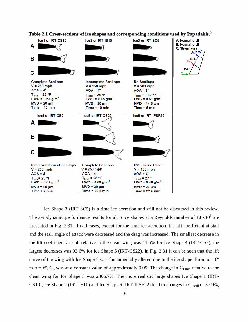
Table 2.1 Cross-sections of ice shapes and corresponding conditions used by Papadakis........... 16

Table 3.1 Geometric Comparison of CRM and UIUC Wind Tunnel Model ................................ 44

Table 3.2 Spanwise location of each tap row and the number of pressure taps. .......................... 45

Table 3.3 Balance Load Range ..................................................................................................... 47

Table 3.4 Range ratios for force balance. ..................................................................................... 47

Table 3.5 Vertical and Horizontal probe stepsize for the various regions. ................................... 50

Table 3.6 Icing conditions input into LEWICE 3.0 ...................................................................... 58

Table 4.1 αStall and CL,Stall for the clean wing. (Stall defined at CM,min) ........................................ 77

Table 4.2 αStall and CL,Stall for the ice wing. (Stall defined at CM,min) ............................................ 77

Table 4.3 Effect of Re on αStall and CL,Stall for the clean wing. (Stall defined at CM,min) ............... 91

Table 4.4 Effect of Re on αStall and CL,Stall for the ice wing. (Stall defined at CM,min) ................... 91

Table E.1 Summary of uncertainties for various quantities. ....................................................... 162

Table E.2 Balance performance coefficient uncertainties. ......................................................... 162

vii

List of Figures

Fig. 2.1 Diagram of swept wing.................................................................................................... 20

Fig. 2.2 Lift coefficient distribution of a straight wing. Adapted from Katz. ............................... 20

Fig. 2.3 Lift coefficient distribution of a swept wing. Adapted from Katz.. ................................ 21

Fig. 2.4 Example of staggered pressure distribution on a swept wing. ........................................ 21

Fig. 2.5 Path of a particle outside of the boundary layer (full line) and inside the boundary layer

(dashed line). ................................................................................................................................. 22

Fig. 2.6 Variation of CM with CL for a family of wings of different sweep angles. AR = 6.0, λ=

0.5, NACA 2415 airfoil. ............................................................................................................... 22

Fig. 2.7 Comparison of 2D and 3D experimental lift curves. ΛLE = 45º, AR = 6, λ = 0.5, NACA

64A010, Re = 8x106, M = 0.2. ...................................................................................................... 23

Fig. 2.8 Sketch of general features of a leading-edge vortex. ....................................................... 23

Fig. 2.9 Sectional lift coefficient curves for a tapered wing. ΛLE= 49º, AR = 3, λ = 0.5, NACA

64A410, Re = 4x106, M = 0.8. ...................................................................................................... 24

Fig. 2.10 Schematic of leading-edge vortex. Figure adapted from Poll. ...................................... 24

Fig. 2.11 Surface oil flow pattern showing spanwise running separation bubble. α = 7º, ΛLE= 30º,

r/c = 0.0003 and Re = 1.7x106. ..................................................................................................... 25

Fig. 2.12 Surface oil flow pattern showing a burst vortex. α = 10º, ΛLE= 30º, r/c = 0.0003 and Re

= 1.7x106. ...................................................................................................................................... 25

Fig. 2.13 Surface oil flow and pressure distributions for a full-span leading-edge vortex. α = 11º,

ΛLE= 56º, r/c = 0.0003 and Re = 2.7x106. ..................................................................................... 26

Fig. 2.14 Surface oil flow showing a part-span leading-edge vortex. α = 11º, ΛLE= 56º, r/c =

0.012, and Re = 2.7x106. ............................................................................................................... 27

Fig. 2.15 Approximate angle of attack for the formation of a spiral vortex. Unit Reynolds number

of 2x106/m. .................................................................................................................................... 28

Fig. 2.16 Details of the flow within the leading-edge vortex near the root of the wing. α = 19º,

ΛLE= 60º. S = Separation, R = Reattachment. .............................................................................. 28

Fig. 2.17 Oil flow Reynolds number comparison. α = 15º, ΛLE= 30º and r/c = 0.03. a) Re =

0.9x106, b) 1.7x10

6........................................................................................................................ 29

viii

Fig. 2.18 Effect of Reynolds number on the lift of a swept wing with ΛLE= 50º. ........................ 29

Fig. 2.19 Effect of Reynolds number and wing leading-edge geometry on inflection lift

coefficient. .................................................................................................................................... 30

Fig. 2.20 Sectional normal force coefficient curves for a wing at different Reynolds numbers.

ΛLE= 49º, AR = 3, λ = 0.5, NACA 64A410 and M = 0.8. .......................................................... 30

Fig. 2.21 Section normal force coefficients for a wing at two different Reynolds numbers. Λc/4=

35º, AR = 5, λ = 0.7, NACA 651A012 (streamwise) and M = 0.25. ............................................ 31

Fig. 2.22 Section normal force coefficients for a wing at two different Reynolds numbers. Λc/4=

35º, AR = 5, λ = 0.7, NACA 651A012 (streamwise) and M = 0.8. .............................................. 31

Fig. 2.23 Horn ice geometry. ........................................................................................................ 32

Fig. 2.24 Effect of horn ice shapes of various heights on Cl and Cm of an NLF 0414 airfoil. Re =

1.8x106, M=0.18 ........................................................................................................................... 32

Fig. 2.25 Sketch and characteristic pressure distribution of a laminar separation bubble. .......... 33

Fig. 2.26 Comparison of pressure distribution for a NACA 0012 with and without a simulated

horn ice shape, α = 4º, Re = 1.5x106 and M = 0.12. ..................................................................... 34

Fig. 2.27 Separation streamlines behind a simulated horn ice shape for various angles of attack,

Re = 1.5x106 and M = 0.12. .......................................................................................................... 34

Fig. 2.28 Photographs of a scallop ice accretion on a wing with ΛLE= 45º. ................................. 35

Fig. 2.29 Ice accretion on a swept wing in glaze icing conditions. Arrows indicate direction of

flow. a) Complete scallops, b) Incomplete scallops, c) No scallops. ............................................ 35

Fig. 2.30 Photographs of ice shapes used by Papadakis et al. for corresponding icing conditions.

....................................................................................................................................................... 36

Fig. 2.31 Aerodynamic coefficients of clean wing and IRT generated ice shapes. a) Lift

Coefficient, b) Drag coefficient, c) Pitching moment coefficient. Re = 1.8x106. ........................ 36

Fig. 2.32 Ice shape simulations for 25% scale T-Tail model. ....................................................... 37

Fig. 2.33 Effect of horn ice simulations on CL of the 25% T-Tail model at Re = 1.36x106

. ........ 37

Fig. 2.34 Cross-section of the ice shape simulation used by Bragg et. al., on a swept NACA 0012.

....................................................................................................................................................... 38

Fig. 2.35 CFD results for swept wing with leading-edge ice accretion. a) Surface oil flow

simulation, b) Particle trajectory simulation. α = 4º, Re = 1.5x106. ............................................. 38

ix

Fig. 2.36 CFD results for swept wing with leading-edge ice accretion. a) Surface oil flow

simulation, b) Particle trajectory simulation. α = 8º, Re = 1.5x106. ............................................. 39

Fig. 2.37 Pressure distributions for swept wing with and without glaze ice accretion. α = 8º, Re

= 1.5 x 106. .................................................................................................................................... 39

Fig. 2.38 (u/U∞) velocity contours on wing upper surface at y/b = 0.40. α = 8º, Re = 1.0x106. .. 40

Fig. 2.39 (u/U∞) velocity contours on wing upper surface at y/b = 0.70. α = 8º, Re = 1.0x106. .. 40

Fig. 2.40 (v/U∞) velocity contours on wing upper surface at y/b = 0.40. α = 8º, Re = 1.0x106. .. 41

Fig. 3.1 Illustration of wind tunnel facility. .................................................................................. 61

Fig. 3.2 Common Research Model. .............................................................................................. 61

Fig. 3.3 Steel frame for wind tunnel model. ................................................................................. 62

Fig. 3.4 Components of SLA shell................................................................................................ 63

Fig. 3.5 Row of pressure taps on the upper surface. ..................................................................... 64

Fig. 3.6 Structural ridges in the interior of the upper surface. ...................................................... 64

Fig. 3.7 Threaded inserts within the structural ridges of the upper surface and the bolt holes on

the lower surface. .......................................................................................................................... 65

Fig. 3.8 Important features of the steel frame. Note that one leading-edge tab is not shown. ...... 66

Fig. 3.9 Leading-edge connected to frame.................................................................................... 67

Fig. 3.10 Photograph of model connected to the force balance. ................................................... 68

Fig. 3.11 Schematic of DTC Initium setup. .................................................................................. 69

Fig. 3.12 Control volume and coordinate system for 3D wake survey......................................... 69

Fig. 3.13Cross-section of the ice shape simulation at the root of the model. ............................... 70

Fig. 3.14 Cross-section of the ice shape simulation at mid span of the model. ............................ 70

Fig. 3.15 Cross-section of the ice shape simulation at the tip of the model. ................................ 71

Fig. 4.1 Oil flow images of clean wing over a range of angles of attack. Re = 3x105 ................. 93

Fig. 4.2 Features of leading-edge vortex. Clean wing, α = 5.5º, Re = 3x105. .............................. 94

Fig. 4.3 Oil flow of the stalled clean wing, α = 9.6º, Re = 3x105. ................................................ 94

Fig. 4.4 Oil flow images of the iced wing over a range of angles of attack. Re = 3x105 ............. 95

Fig. 4.5 Features of leading-edge vortex. Iced wing, α = 5.5º, Re = 3x105. ................................. 96

Fig. 4.6 Reattachment line of the separated flow on the iced wing for a range of angles. Re =

3x105. ............................................................................................................................................ 96

Fig. 4.7 Oil flow of the stalled iced wing, α = 6.5º, Re = 3x105. .................................................. 97

x

Fig. 4.8 Force balance results for the clean and iced wing. .......................................................... 98

Fig. 4.9 Change in a) Lift coefficient and b) drag coefficient due to ice shape. ........................... 99

Fig. 4.10 Comparison of total lift and drag for the clean wing measured by the force balance and

by the wake survey technique. Re = 6x105 ................................................................................. 100

Fig. 4.11 Comparison of total lift and drag for the iced wing measured by the force balance and

by the wake survey technique. Re = 6x105 ................................................................................. 101

Fig. 4.12 Profile and induced drag for the clean and iced wing. Re = 6x105 ............................. 102

Fig. 4.13 Comparison of clean and iced wing oil flow. α = 3.3º, Re = 6x105 ............................ 102

Fig. 4.14 Comparison of clean and iced wing CP distributions for rows 1-4. α = 3.3º, Re = 6x105

..................................................................................................................................................... 103

Fig. 4.15 Wakes of the a) clean wing and b) iced wings at α = 3.3º, Re = 6x105. Contours of

u/U∞. Vectors represent transverse velocity. ............................................................................... 104

Fig. 4.16 Oil flow and wake of iced wing. α = 3.3º, Re = 6x105. Contours of u/U∞. ................. 105

Fig. 4.17 Comparison of clean and iced wing sectional a) lift, b) drag, c) profile drag and d)

induced drag coefficients. α = 3.3º, Re = 6x105 ......................................................................... 106

Fig. 4.18 Contours of normalized streamwise vorticity in the wake of the iced wing. α = 3.3º, Re

= 6x105. ....................................................................................................................................... 107

Fig. 4.19 Comparison of clean and iced wing oil flow. α = 5.5 º, Re = 6x105 ........................... 107

Fig. 4.20 Comparison of clean and iced wing CP distributions for rows 1-4. α = 5.5º, Re = 6x105

..................................................................................................................................................... 108

Fig. 4.21 Wakes of the a) clean wing and b) iced wings at α = 5.5º, Re = 6x105. Contours of

u/U∞. Vectors represent transverse velocity. ............................................................................... 109

Fig. 4.22 Oil flow and wake of the iced wing at α = 5.5º and Re = 6x105. Contours of u/U∞.

Vectors represent transverse velocity. Reattachment line of the leading-edge vortex is

highlighted. ................................................................................................................................. 110

Fig. 4.23 Contours of normalized streamwise vorticity in the wake of the iced wing. α = 5.5º, Re

= 6x105. ....................................................................................................................................... 110

Fig. 4.24 Comparison of clean and iced wing sectional a) lift, b) drag, c) profile drag and d)

induced drag coefficients. α = 5.5º, Re = 6x105 ......................................................................... 111

Fig. 4.25 Stalled flowfield comparison of clean and iced wing oil flow. Re = 6x105 ................ 112

xi

Fig. 4.26 Comparison of clean and iced wing CP distributions for rows 1-4. Both wings beyond

stalling angle of attack. Clean wing α = 10.7º, Iced wing α = 6.5º, Re = 6x105 ........................ 113

Fig. 4.27 Wakes of the stalled clean and iced wing. Clean wing α = 10.7º, Iced wing α = 6.5º, Re

= 6x105. Contours of u/U∞. Vectors represent transverse velocity. ............................................ 114

Fig. 4.28 Comparison of stalled clean and iced wing sectional a) lift, b) drag, c) profile drag and

d) induced drag coefficients. Clean wing α = 10.7º, Iced wing α = 6.5º, Re = 6x105. ............... 115

Fig. 4.29 Comparisons of pre and post-stall Cl distributions for the a) clean and b) iced wings. Re

= 6x105 ........................................................................................................................................ 116

Fig. 4.30 Oil flow of the clean wing, 0.68 ≤ 2y/b≤ 1, at two different Reynolds numbers. α =

3.3º. ............................................................................................................................................. 117

Fig. 4.31 Oil flow of the iced wing, 0.68 ≤ 2y/b≤ 1.0, at two different Reynolds numbers. α =

3.3º. ............................................................................................................................................. 117

Fig. 4.32 Oil flow of the clean wing, 0.625 ≤ 2y/b≤ 0.925, at two different Reynolds numbers. α

= 7.6º ........................................................................................................................................... 118

Fig. 4.33 Oil flow of the ice wing, 0.45 ≤ 2y/b≤ 0.75, at two different Reynolds numbers. α= 5.5º

..................................................................................................................................................... 118

Fig. A.1 Pressure port numbering convention ............................................................................ 132

Fig. A.2 Probe coordinate system and flow angle definition. ..................................................... 132

Fig. A.3 Probe mounted in the tunnel during calibration. .......................................................... 133

Fig. A.4 Aluminum rod used as base of the probe support. ........................................................ 133

Fig. A.5 Manual rotation stage used to set the roll angle of the probe. ...................................... 134

Fig. A.6 Probe holder and adaption plate mounted to the rotation stage. ................................... 134

Fig. A.7 Probe mounted in probe holder..................................................................................... 135

Fig. A.8 Five-hole probe calibration surface for at Rep = 10762 ......................................... 136

Fig. A.9 Five-hole probe calibration surface for at Rep = 10762 ......................................... 136

Fig. A.10 Five-hole probe calibration surface for at Rep = 10762 ..................................... 137

Fig. A.11 Five-hole probe calibration surface for at Rep = 10762 ...................................... 137

Fig. A.12 Difference between actual flow angles and angles determined from calibration

surfaces. Rep = 10762 ................................................................................................................. 138

xii

Fig. A.13 Difference between actual pressure coefficients and those determined from calibration

surfaces. Rep = 10762 ................................................................................................................. 138

Fig. A.14 Difference between actual and measured flow angles. Measurements taken at Rep =

5381, calibration Rep = 10762 .................................................................................................... 139

Fig. B.1Control volume used in the derivation of the wake survey equations. .......................... 147

Fig. C.1 Normalized streamwise vorticity over the entire measurement plane. Clean wing, α = 4º,

Re = 6x105. ................................................................................................................................. 152

Fig. C.2 Normalized streamwise vorticity in the wake. Clean wing, α = 4º, Re = 6x105. .......... 152

Fig. C.3 Total pressure coefficient over the entire measurement plane. Clean wing, α = 4º, Re =

6x105. .......................................................................................................................................... 153

Fig. C.4 Total pressure coefficient in the wake. Clean wing, α = 4º, Re = 6x105. ..................... 153

Fig. C.5 Conceptual schematic of computational domain. ......................................................... 154

Fig. C.6 Effect of error tolerance in the calculation of ψ on the induced drag of the clean and iced

wing. α = 4º, Re = 6x105. ............................................................................................................ 155

Fig. D.1 Comparison of uncorrected and corrected lift coefficient plotted against the uncorrected

angle of attack. Clean wing, Re = 6x105 ..................................................................................... 158

Fig. D.2 Comparison of uncorrected and corrected drag coefficient for the clean wing plotted

against the uncorrected angle of attack. Clean wing, Re = 6x105 .............................................. 158

Fig. D.3 Comparison of uncorrected and corrected pitching moment coefficient for the clean

wing plotted against the uncorrected angle of attack. Clean wing, Re = 6x105 ........................ 159

Fig. D.4 Comparison of uncorrected lift coefficient plotted against the uncorrected and the

corrected angle of attack. Clean wing, Re = 6x105 ..................................................................... 159

xiii

Nomenclature

AR Aspect ratio

Ass Wind tunnel settling section area

Ats Wind tunnel test section area

b/2 Semispan

cmac Mean aerodynamic chord

c(y) Local chord distribution

Cα 5-hole probe pitch coefficient

Cβ 5-hole probe yaw coefficient

Cd Sectional drag coefficient

Cdi Sectional induced drag coefficient

Cdp Sectional profile drag coefficient

Cl Sectional lift coefficient

CD Drag coefficient

CDi Induced drag coefficient

CDo Minimum drag coefficient

Cp Model surface pressure coefficient

Cp,s Static pressure coefficient in the wake

Cp,t Total pressure coefficient in the wake

CPs Static pressure calibration coefficient

CPt Total pressure calibration coefficient

CL Lift coefficient

CL,Stall Lift coefficient at the stalling angle of attack

CM Quarter-chord pitching moment coefficient

D Drag

DCpt Total pressure loss coefficient

Di Induced drag

Dp Profile drag

FA Axial force measured by balance

FN Normal force measured by balance

Kλ Taper correction factor

L Lift

M Pitching moment about the center of the balance

Mc/4 Quarter chord pitching moment

M∞ Freestream Mach number

P Static pressure

xiv

Pamb Ambient Pressure

Pavg Average of pressures measured by ports 2-5 on the 5-hole probe

Pi Pressure measured by the ith

pressure port on the 5-hole probe

Pss Static pressure in settling section

Pt Total pressure in the wake

Pt∞ Freestream total pressure

Pts Static pressure in test section

q∞ Dynamic pressure

R Ideal gas constant for air

Re Reynolds number based on mean aerodynamic chord

S Model planform area

Tamb Ambient temperature

u Streamwise velocity in the wake

ub Wake blockage velocity

u’ Perturbation velocity

u* Artificial velocity

Uss Settling section velocity

Uts Test section velocity

U∞ Freestream velocity

v Spanwise velocity in the wake

VA Scaled axial force voltage

VM Scaled pitching moment voltage

VN Scaled normal force voltage

Vtotal Total velocity measured by the 5-hole probe

w Normal velocity in the wake

x Streamwise direction

y Spanwise direction

z Normal direction (positive from lower to upper surface)

ΔCDup Drag coefficient correction for boundary induced upwash

ΔCMsc Pitching moment coefficient for streamline curvature

ΔUsb Velocity increment due to solid blockage

ΔUwb Velocity increment due to wake blockage

xv

Greek Symbols

α Model angle of attack (measured at the root)

αp 5-hole probe pitch angle

αStall Model angle of attack at stall

βp 5-hole probe yaw angle

δ Upwash interference parameter for a swept wing

δ’ Upwash interference parameter assuming no taper

εsb Non-dimensional velocity increment due to solid blockage

εtotal Non-dimensional velocity increment due to the total blockage

εwb Non-dimensional velocity increment due to wake blockage

Γ(y) Spanwise circulation distribution

λ Taper ratio

ΛLE Leading-edge sweep angle

Λc/4 Quarter-chord sweep angle

ϕ Velocity potential in the transverse plane or 5-hole probe roll angle

ψ Stream function in the transverse plane

ρ Air density

σ Transverse source term

θ 5-hole probe cone angle

τ2 Streamline curvature correction factor

μ Dynamic viscosity

ξ Streamwise vorticity

Δαsc Angle of attack correction due to streamline curvature

Δαup Angle of attack correction due to boundary induced upwash

1

Chapter 1

Introduction

After decades of research, airframe icing continues to present a significant challenge to

aircraft designers and manufacturers. The accretion of ice, especially on lifting surfaces, can

have serious consequences for an aircraft, as even small ice accretions can lead to a significant

decrease in maximum lift, increase in drag and loss of control authority. A vast amount of

research has been performed that investigated the effects of ice on the aerodynamics of 2D

airfoils. In 2001, Lynch and Khodadoust1 reviewed the effects of ice on the performance of

lifting surfaces. Typical performance penalties on airfoils included 10-50% reduction in

maximum lift, increases in the drag coefficient ranging from 0.01 to 0.1 and 1º-7º reduction in

the stalling angle of attack. The magnitude of the performance penalties are known to depend on

a number of features including the size and shape of the ice accretion, airfoil geometry and the

location at which the ice forms. The results summarized by Lynch and Khodadoust1 provide a

valuable source of information for aircraft designers and certification officials. In 2005, a review

by Bragg et. al.2 discussed the underlying flowfield features that are responsible for the measured

performance degradations. The flowfield of a large leading-edge ice accretion is generally

dominated by a large separation bubble forming behind the ice. This bubble modifies the surface

pressure distribution and results in decreased circulation and increased pressure drag.

Experimental measurements have shown that the size of the separation bubble increases with

angle of attack and can extend to 50% of the chord before the flow fails to reattach. Previous

research has also shown that iced flowfields can be highly unsteady and can generate fluctuations

in the lift coefficient on the order of 10% of the mean. In addition to reviewing the flowfields of

iced airfoils, Bragg et. al.2 proposed a useful ice accretion classification system based on the

aerodynamic effects of the ice.

These reviews demonstrate that the aircraft community has a very thorough

understanding of the effects of ice on the aerodynamics of airfoils. However, aircraft are not two-

dimensional and in order to fully understand aircraft icing it is necessary to extend our

knowledge to three-dimensional lifting surfaces. In particular, an important area of investigation

relevant to many aircraft is the effects of ice on the aerodynamics of swept wings. Swept wing

icing presents a challenging problem due to the large number of variables involved and the

2

complexity of the flow. Compared to airfoils, several new geometric features must be considered

including sweep angle, aspect ratio, taper ratio and twist as well as changes in airfoil geometry

along the span. Spanwise variations in the ice accretion geometry must also be considered. In

addition to the geometry, the flowfield of a clean swept wing is considerably more complex than

an airfoil. Three-dimensional effects modify the local aerodynamics by creating a spanwise

distribution of lift and drag as well as altering the chordwise loading on individual sections.3 This

change in the chordwise loading is known as induced camber and effects the 2D pressure

distribution of the local airfoil. In addition, the sweep angle staggers the local pressure

distributions creating a spanwise pressure gradient resulting in spanwise flow within the

boundary layer.4 These three-dimensional effects lead to spanwise variations in the stalling

characteristics which can have important implications for the overall performance. The

aerodynamics of swept wings are more thoroughly discussed in Chapter 2.

Compared to airfoils, there is relatively little published research on the effects of ice on

swept wings and as a result the aerodynamics are poorly understood. Papadakis et. al.5,6

measured the performance effects of various ice accretions on a swept wing with ΛLE = 28º, AR

= 6.8 and λ = 0.4 and a modern transonic airfoil. Force balance measurements showed decreases

in lift as high as 93.6% with a corresponding increase in drag of 3500%. Surface pressure

distributions suggested the presence of a large leading-edge vortex due to separation from the tip

of the ice shape. Unfortunately, other than the pressure distributions there were no flowfield data.

Khodadoust and Bragg7 and Bragg et. al.

8 used several experimental methods including pressure

measurements, surface oil flow, helium bubble flow visualization and LDV to study the

flowfield of an iced swept wing with ΛLE = 30º, AR = 2.3 and λ = 1.0 with a NACA 0012 airfoil.

The experimental results showed that the flowfield was dominated by a leading-edge vortex that

grew as the angle of attack increased and was eventually shed into the wake as the wing stalled.

While these results were very insightful, the simple geometry used was not representative of

modern aircraft.

A drawback common to the investigations by Papadakis et. al.5,6

and Bragg et. al.7,8

was

the small scale of the models and the low Reynolds numbers at which the tests were performed.

There is currently no aerodynamic performance or flowfield data for iced swept wings at

Reynolds numbers representative of flight. It is difficult to obtain high Reynolds number data on

swept wings due to the small scale of the models and limited availability and high costs of large

3

pressurized wind tunnels. There is currently considerable interest in obtaining high Reynolds

number data for an iced swept wing. The University of Illinois, the FAA, NASA, ONERA and

Boeing are currently working together on various aspects of a major project aimed at acquiring

high Reynolds number data on a swept wing model that is representative of the wings of modern

commercial airliners. The overall goal of the project as described by Broeren9 is to: “Improve the

fidelity of experimental and computational simulation methods for swept wing ice accretion

formation and the resulting aerodynamic effect.” A major objective of this project is to improve

our understanding of the aerodynamic effects of ice on swept wings. This includes Reynolds and

Mach number effects, the underlying flowfield physics and differences from the 2D case. In

addition, a database of high Reynolds experimental results is an important step towards

determining the level of geometric fidelity required to accurately simulate swept wing icing

effects.

The work described in this thesis represents a preliminary step towards the goal of

obtaining high Reynolds number data for an iced swept wing. Previous 2D and 3D icing research

suggests that the aerodynamics of iced swept wings will be highly three-dimensional and

complex, and it will require more than just force balance data to fully understand the

performance and the underlying flowfield physics. In order to accomplish the goals of the overall

project it will be necessary to utilize several different experimental techniques. However, as

mentioned above, time is limited in high Reynolds number tunnels, so before this testing can

begin it is important to carefully select which experimental techniques should be used.

The goal of this thesis is to investigate and demonstrate the use of various experimental

methods applied to understanding the performance and flowfield of a highly swept, high-aspect

ratio wing with a simple ice shape simulation at low Reynolds numbers. The methods used in

this work include force balance measurements, surface pressure measurements, surface oil flow

visualization and 5-hole probe wake surveys. These methods represent several possible

techniques that can be used in larger tunnels, and this work will demonstrate how the results of

these methods can be used together in order to obtain a more complete picture of the

aerodynamics of the iced swept wing used in this study. Force balance measurements will

provide performance data while the surface oil flow will identify key flowfield features. The

wake survey will be used to determine the effect of ice on the profile and induced drag as well as

the spanwise distribution of the loads, and changes in the load distribution will be related to

4

features observed in the flow. All experiments performed for this work were done at low

Reynolds number and the data are not intended to represent the aerodynamics of the swept wing

in flight. The purpose of this work is only to demonstrate how these experimental methods can

be used to improve our understanding of iced swept wing aerodynamics.

The layout of this thesis is as follows. Chapter 2 will provide a detailed background and

review of literature of several topics related to the work presented in this thesis. Topics include

swept wing aerodynamics including stall and Reynolds number effects, a brief review of iced

airfoil aerodynamics and finally a more thorough review of the iced swept wing aerodynamics

literature. Chapter 3 will provide a detailed description of the various experimental techniques

utilized in this work. Finally, Chapter 4 will present the results of these techniques and use the

data to describe the performance and flowfield of the swept wing at low Reynolds number.

5

Chapter 2

Background

This chapter will provide a background of various topics related to this research. This

review will begin with a discussion on swept wing aerodynamics including the stalling process,

the formation of leading-edge vortices and Reynolds number effects. This will be followed by a

brief review of iced airfoil and iced swept wing aerodynamics. The purpose of this chapter is to

provide a basis for understanding the results presented in subsequent chapters.

2.1 Swept Wing Aerodynamics

Swept wings are the result of a compromise between high and low-speed performance.

The primary advantage of the swept wing is to delay the drag rise due to shock formation to

higher subsonic Mach numbers. This delay in the drag rise is possible because the formation of

shock waves is dependent on the component of velocity normal to the leading-edge of the wing,

and this velocity component decreases with the cosine of the sweep angle.10

Figure 2.1

demonstrates this concept while also labeling the important geometric features of the swept

wing. Swept wings are therefore important for high-speed cruise conditions of typical

commercial airliners, but this improved high-speed performance generally comes at the expense

of low-speed performance as the lift curve slope is generally decreased and the induced drag is

increased.4,10

The results to be presented in this thesis, and much of the work to be done for the overall

project, will be concerned with the performance of swept wings at low speeds, below M∞ = 0.3.

This speed range will be the focus of this review. The performance of swept wings at low

subsonic Mach numbers depends on numerous geometrical features of the wing as well as the

flight conditions. This review will begin by discussing how swept wings differ from straight

wings under normal flight conditions; this will be followed by the stalling characteristics of

swept wings and finally the effects of Reynolds number.

2.1.1 Characteristics of Swept Wing Aerodynamics

For high aspect ratio straight wings, the primary difference between the wing and airfoil

flowfield is the existence of the tip vortices. These vortices induce a downwash across the wing

6

which effectively reduces the local angle of attack of each section and as a result the lift curve

slope of the wing is less than that of the airfoil.10

Due to the presence of the wing tips, the lift

distribution is not constant across the entire span; this is demonstrated in Fig. 2.2 which shows a

typical lift distribution for a simple straight wing. It can be seen that the lift is highest in the

center and monotonically decreases to zero at the tip. In the case of a swept wing, in addition to

the tip vortices inducing a downwash across the span, each section of the wing induces an

upwash in front of each downstream section. The net result for an untwisted swept wing is an

increase in the effective angle of attack at the outboard sections relative to the inboard

sections.4,10

This has the effect of shifting the lift distribution outboard as shown in Fig. 2.3. This

will have important implication for the stalling characteristics of swept wings as will be seen

shortly.

In addition to modifying the spanwise load distribution, sweep has an important effect on

both the chordwise and spanwise pressure gradients. Induced camber refers to the altering of the

chordwise loading of a section of the wing.3 On a swept wing, the induced camber is negative at

the tip and positive at the root.3,11

This results in increased pressure gradients near the leading-

edge of the tip sections and a reduction in the adverse pressure gradient of the root sections. The

spanwise pressure gradient also plays a very important role in aerodynamic characteristics of

swept wings. As can be seen in Fig. 2.4, from Hoerner,4 the sweep staggers the pressure

distributions along the span. As a result of this staggering a spanwise pressure gradient is

established. For example in Fig. 2.4, if a fluid particle is located at spanwise section AA and

streamwise station (a) the pressure increase from AA to BB along the line (a) is greater than the

increase from streamwise station (a) to (b). The balance between the particle’s inertia and the

pressure forces result in a trajectory that is primarily in the streamwise direction and slightly

inboard. At streamwise station (c) however this is no longer the case. Now the pressure decreases

from section AA to BB along the line (c) but is still increasing in the streamwise direction. A

fluid particle outside of the boundary layer has sufficient momentum to continue moving

primarily in the streamwise direction; however, a particle in the boundary layer, having lost

much of its momentum, will now begin traveling towards the tip. Figure 2.5 shows the path of

the two particles, one outside of the boundary layer and the other inside. The spanwise pressure

gradient establishes a significant spanwise flow in the boundary layer flow from the root to the

tip. These features of swept wings; shifting of the load to outboard sections, induced camber

7

increasing adverse pressure gradients at the outboard sections and the existence of spanwise flow

in the boundary layer have very important implications for the stalling characteristics of swept

wings.

2.1.2 Swept Wing Stall

An important feature of swept wing performance is the manner in which the wing stalls.

The stalling process is especially important when studying aircraft icing because the presence of

ice has the potential to drastically alter when the wing stalls and the manner in which it stalls.

Like airfoils,12

there are several mechanisms which can lead to stall on swept wings. The two

fundamental causes of stall on a swept wing are leading-edge and trailing-edge separation.

Furlong and McHugh3 pointed out that while distinct, these stall types may occur

simultaneously, and which stall type dominates depends on the wing geometry and Reynolds

number.

Before discussing the stalling process in more detail, it is important to note a feature

common to nearly all swept wings regardless of the dominate stalling mechanism. A major

disadvantage of swept wings, compared to straight wings, is their tendency to stall at the tip

before the root.3,4,13

This is a disadvantage for several reasons. When a swept wing stalls at the

tip there is a forward shift in the center of pressure resulting in an increase in the pitching

moment. An increase in pitching moment is unstable and leads to a further increase in the angle

of attack unless proper control is applied. This is demonstrated in Fig. 2.6, from Anderson,14

which shows CL versus CM for three wings with different sweep angles and a NACA 2415

airfoil, AR = 6 and λ = 0.5. It can be seen that for the sweep angles of 0º and 15º the pitching

moment decreases when the wing stalls, but when the sweep angle is increased to 30º the

outboard sections stall first resulting in a more positive pitching moment. In addition to the

unstable change in pitching moment, control surfaces such as ailerons are generally located on

the outboard sections so stall in these regions will result in loss of control authority. By properly

designing the wing, by adding taper and twist for example, it is possible to prevent tip stall.

The main reasons for tip stall occurring first are higher local lift coefficients on the

outboard sections, the spanwise flow from the boundary layer to the tip and lower local Reynolds

number if the wing is tapered. As seen in Fig. 2.2 the local sectional lift coefficient of the straight

wing is maximum in the center of the wing, as a result a straight wing tends to stall near the root

8

first. The sectional lift coefficients on the outboard sections of a swept wing are typically higher

than the inboard sections, as shown in Fig. 2.3, and therefore are more susceptible to stall.

Spanwise flow in the boundary, flowing from the root to the tip, acts as a form of suction for the

inboard sections making them very resistant to stall, while at the same time increasing the

thickness of the boundary layer on the outboard sections.3,4,13

In many cases the sectional lift

coefficient on the inboard sections can be far greater than the maximum lift coefficient of the 2D

airfoil. A comparison of 2D and 3D sectional lift curves for several spanwise stations of a 45˚

swept wing at a Reynolds number of 8x106 is shown in Fig. 2.7.

15 It can be seen that the

maximum sectional lift coefficients inboard of the tip far exceed those of the airfoil. This

increase in sectional lift coefficients is attributable to the spanwise flow.

As mentioned previously, the tendency for outboard sections to stall first independent of

whether the local sections stall at the leading-edge, trailing-edge or a combination of both. When

trailing-edge stall dominates, the spanwise flow in the boundary layer from root to tip leads to an

excessively thick boundary layer near the trailing-edge in the tip region. At the same time the

spanwise flow makes the boundary layer of the inboard sections resistant to trailing-edge

separation. The thick boundary layer of the outboard sections begins to separate near the trailing-

edge and the point of separation slowly moves forward with increasing angle of attack.

While the spanwise flow is particularly effective at delaying trailing-edge separation of

the inboard sections, if it is strong enough trailing-edge separation may also be suppressed for

outboard sections. In this case leading-edge separation may occur.3,13

Leading-edge separation

may also occur for thinner wings where the adverse leading-edge pressure gradient is larger.

Leading-edge separation will likely start at the outboard sections because these sections are at a

higher local angle of attack and the induced camber is such that the adverse pressure gradient

near the leading-edge is increased relative to the 2D airfoil section.3,11

A very important

difference between leading-edge stall of swept wings and airfoils is the presence of a spanwise

vortex. Leading-edge separation can lead to the formation of separation bubbles and the

spanwise pressure gradient converts this bubble into the well-known leading-edge vortex.12,13,16

At a sufficiently high angle of attack the leading-edge vortex will start inboard of the tip, grow in

diameter as it travels outboard and eventually being shed into the wake inboard of the tip. This is

illustrated in a sketch from Polhamus16

shown in Fig. 2.8.

9

The leading-edge vortex can have significant effects on the performance of the swept

wing. The high rotational velocities within the vortex alter the pressure field and induce non-

linear changes in the lift. This non-linearity is demonstrated in Fig. 2.9, adapted from Boltz and

Kolbe17

, for a wing with ΛLE= 49º, AR = 3, λ = 0.5, Re = 4x106, M = 0.8. It can be seen that at

each spanwise station there is an angle of attack at which the slope of the normal force

coefficient increases substantially, this change in slope is a direct result of the low pressures

induced on the surface by the vortex. Similar features can be seen in the lift curves shown in Fig.

2.7.

2.1.3 Leading-Edge Vortex Flowfield

When a leading-edge vortex occurs it can dominate the flowfield of the swept wing.

Poll18

used surface oil flow visualization and surface pressure taps to investigate the formation

and development of the leading-edge vortex on a swept wing for various combinations of wing

geometry, angle of attack and Reynolds number. A sketch of the fundamental features of the

leading-edge vortex as described by Poll is shown in Fig. 2.10. First a separated shear layer is

formed at the primary separation line located near the leading-edge. The shear layer rolls up to

form a vortex, and the flow over the vortex attaches to the surface at the reattachment line.

Downstream of the reattachment line the boundary layer moves towards the trailing-edge likely

with a significant spanwise component. Upstream of the reattachment line, the boundary layer

under the vortex moves upstream towards the leading-edge. The approximate location of the core

of the vortex is given by the line connecting the inflection points of the surface oil lines.19

As the

boundary layer flows from the reattachment line to the line indicating the vortex core it

experiences a favorable pressure gradient due to the low pressure in vortex core. After passing

the vortex core the boundary layer is now in an adverse pressure gradient and eventually

separates from the surface at the secondary separation line. This new shear layer is entrained into

the shear layer originating from the primary separation line.

Poll examined the surface flow for wings of various angles of attack, leading-edge radii,

sweep angles, and Reynolds numbers. Beginning at an angle of attack of 3.5º for a wing with

ΛLE = 30º, r/c = 0.0003 and Re = 1.7x106

a quasi-two-dimensional separation bubble formed

along the entire span of the model. Oil flow representing this structure at α = 7º is shown in Fig.

2.11. The location of the reattachment line moved downstream as the angle of attack increased

10

until the vortex burst which is shown in Fig. 2.12 for an angle of attack of 10º. In the case of the

burst vortex, the reattachment line terminated part way across the span. Outboard of where the

reattachment line ended the oil showed that the spanwise flow near the trailing-edge was towards

the tip, but near the leading-edge this spanwise flow was towards the root. The result of this

inboard moving spanwise flow was an area of oil accumulation indicated by the dark spot.

When the sweep angle was increased the flowfield remained qualitatively similar to that

shown in Fig. 2.11 for low angles of attack. However at higher angles of attack a full-span

leading-edge vortex formed. The leading-edge vortex of the wing at α = 11º with ΛLE = 56º, r/c =

0.0003 and Re = 2.7x106 is shown in Fig. 2.13; surface pressure distributions at three spanwise

locations are also shown. The vortex originated at the root of the wing, grew in diameter as it

moved outboard and curved away from the leading-edge and was shed into the wake inboard of

the tip. In the pressure distributions, suction peaks can be observed at x/c of approximately 0.2,

0.3 and 0.5 for the root, center and tip respectively. The suction peaks correspond to the

approximate location of the vortex core. The magnitude of the suction peak decreased as the tip

was approached, because as the vortex grew the rotational velocities decreased causing an

increase in pressure. The region of constant pressure near the leading-edge was due to the

secondary separation seen in the oil flow.

In addition to the formation of a full-span separation bubble or leading-edge vortex, Poll

also observed part-span leading-edge vortices. By increasing the leading-edge radius of the wing

in Fig. 2.13 to r/c = 0.012 the flowfield shown in Fig. 2.14 was formed. Here it can be seen that a

full-span short bubble was formed, the downstream boundary of the bubble is marked by the first

reattachment line. On the inboard sections of the wing the flow remained attached downstream

of the bubble. On the outboard sections the flow separated again downstream of the bubble at the

secondary separation line. The new shear layer rolled up to form a part-span vortex and the flow

reattached at the secondary reattachment line. The spanwise flow downstream of the secondary

reattachment line separated again along the tertiary separation line near the tip.

Figure 2.15 shows the approximate angle of attack at which a leading-edge vortex first

formed versus the sweep angle for three different leading-edge radii at a unit Reynolds number

of 2x106/m. The formation of the leading-edge vortex was first observed for a sweep angle of

30º. It can be seen that the angle of attack corresponding to vortex formation decreased with

leading-edge radius and in general decreased with increasing sweep angle.

11

Mirande et. al.19

performed flow visualization in both a wind and water tunnel on a

simple low aspect ratio swept wing with a symmetrical airfoil. Figure 2.16 shows a sketch of

flow visualization results near the root of the wing, ΛLE = 60º and α = 19º Cross-sections of the

leading-edge vortex are shown for several spanwise locations, separation lines are marked S and

reattachment lines are marked R. It can be seen that as the tip was approached the reattachment

line moved downstream and the diameter of the vortex increased. For the first two spanwise

stations there were no secondary separation lines. At the third station shown in the figure there

was a secondary separation point marked S2 and a smaller secondary vortex with rotation

opposite that of the main vortex began at S2. This is different from Poll’s interpretation of the

secondary separation line shown in Fig. 2.10. In Poll’s description, the shear layer forming at the

secondary separation line was entrained into the primary shear layer originating from the primary

separation line.

2.1.4 Reynolds Number Effects

The Reynolds number influences the state of the boundary layer and therefore can

significantly impact the performance of the wing. Relative to airfoils there are several additional

geometric variables which can influence the importance of the Reynolds number. The most

important features are likely the airfoil of the wing and the sweep angle. In addition to the

increased number of geometric variables there are several additional routes through which the

boundary layer on a swept wing may transition from laminar to turbulent. Excluding roughness

and external disturbances, transition on an airfoil is generally the result of a laminar separation

bubble or the boundary-layer instability known as Tollmien-Schlicting waves. In addition to

these mechanisms, swept wing boundary layers can also transition due to crossflow instability

and attachment line transition.20

These mechanisms will not be discussed in detail and are only

mentioned here to demonstrate the complexity of Reynolds number effects. The remainder of

this section will focus on how the Reynolds number affects the performance and flowfield of

wings experiencing leading-edge stall and a leading-edge vortex as this case is most relevant to

the current research. Unless otherwise noted the Reynolds number is based on the mean

aerodynamic chord measured in the streamwise direction.

In addition to assessing the effects of wing sweep and leading-edge radius on the

formation of the leading-edge vortex, Poll18

also investigated the effects of Reynolds number.

12

Figure 2.17 shows surface oil flow for a wing at two different Reynolds numbers of 0.9x106 and

1.7x106 both at α = 15º with ΛLE = 30º and r/c = 0.03. At the lower Reynolds number a small

part-span leading-edge vortex was observed near the root, followed by an oil accumulation area

and then reversed flow terminating at the secondary separation line. There was a large region of

separated flow upstream of the secondary separation line and the chordwise extent of this region

increased as the tip was approached. For the higher Reynolds number no part-span vortex was

formed. Instead a part-span short bubble existed on the inboard sections. This bubble terminated

in an oil accumulation area located at midspan.

Polhamus16

presented results showing the effect of Reynolds number on the angle of

attack at which a leading-edge vortex formed. In Fig. 2.18 the lift coefficient versus angle of

attack for a swept wing with ΛLE = 50º at several Reynolds numbers is shown. The formation of

the leading-edge vortex corresponded to the increase in the lift curve slope which resulted from

additional vortex lift. For all three Reynolds numbers the lift curve was bounded by inviscid

theory and Polhamus’s leading-edge suction analogy.21

It can be seen that as the Reynolds

number was increased the formation of the leading-edge vortex was delayed to higher angles of

attack.

Poll18

also investigated the effect of Reynolds number on the angle of attack at which a

leading-edge vortex formed and found that the leading-edge radius plays an important role. In

general the results showed that the larger the leading-edge radius the larger the dependence on

Reynolds number. Furlong and McHugh3 made similar observations when comparing Reynolds

number effects on two swept wings each with Λc/4 = 50º, AR = 2.9 and λ = 0.625. The airfoil of

one wing was made up of two circular arcs and had a sharp leading-edge while the other wing

had a NACA 641-112 section. Figure 2.19 shows the inflectional lift coefficient versus Reynolds

number for the two wings. The inflectional lift coefficient refers to lift coefficient at which the

pitching moment begins to increase and is an indicator of separated flow. It can be seen that for

the wing with the NACA airfoil section the Reynolds number effect was quite large, CL,inflection

more than doubled over the range of Reynolds numbers tested. For the wing with a circular arc

airfoil, that had a sharp leading-edge, the Reynolds number had no effect. This is not surprising

given that a sharp leading-edge will fix the separation location and therefore the Reynolds

number effect will decrease. Similar trends are also observed on delta wings.

13

On a swept wing the effects of Reynolds can vary across the span. The sectional normal

force coefficient curves of the wing in Fig. 2.9 are shown again in Fig. 2.20 at two Reynolds

numbers of 4x106 and 8x10

6. The figure shows that the Reynolds number effect on the outboard

sections was greater than on the inboard sections. The maximum normal force coefficient for the

outboard 30% of the wing changed significantly when the Reynolds number doubled, whereas

the change for the inboard sections was small. For both Reynolds numbers, Cn began to increase

non-linearly at higher angles of attack; however, for the higher Reynolds number this non-linear

increase was more dramatic for the outboard sections. This suggests that the strength of the

vortex increased significantly with Reynolds number. The results of Tinling and Lopez22

also

showed that the effects of Reynolds number were more significant for the outboard sections.

They tested a wing with Λc/4= 35º, AR = 5, λ = 0.7, and a NACA 651A012 section in the

streamwise direction. The wing was tested over a wide range of Reynolds numbers and Mach

numbers which were varied independently. Figure 2.21 shows the normal force coefficients

versus angle of attack for various spanwise stations at Reynolds numbers of 2x106 and 10x10

6

for a constant Mach number of 0.25. Results for Reynolds numbers of 2x106 and 4.3x10

6 at a

Mach number of 0.80 are shown in Fig. 2.22. In both cases it is clear that the effects of Reynolds

number are greater for the outboard section. For M=0.25 the maximum normal force was nearly

doubled for the tip section. For the case of M = 0.8 the maximum normal force was not

significantly changed but the stall type of the outboard sections was altered. For the low

Reynolds number there was a an abrupt drop in Cn typical of leading-edge stall, and for the high

Reynolds number there was a gradual leveling off of Cn typical of thin airfoil stall.12

For a swept wing, the decreased influence of the Reynolds number on the inboard

sections is likely a general result, and is due to the spanwise flow acting as a form of boundary-

layer suction for the inboard sections of the wing. It is possible that the Reynolds number

influences the maximum lift of these inboard sections however due to the spanwise flow the

maximum lift occurs at angles of attack well beyond where the wing has stalled. As a result, the

influence of the Reynolds number on the overall performance of the wing is primarily due to the

effects on the outboard sections of the wing.

14

2.2 Iced Airfoil Aerodynamics

Before discussing past research of iced swept wing aerodynamics a brief review of the

effects of ice on airfoil aerodynamics will be given. There are four primary classifications of ice

accretions that form on airfoils; roughness, streamwise, horn and spanwise ridge ice.2 The horn

ice classification is the most relevant to the current work and will be the focus of this review.

The primary geometric characteristics of a horn ice shape are the height, the angle it makes with

respect to the chord line and its location (s/c) on the surface, see Fig. 2.23. A horn ice accretion

can have a significant effect on the performance of an airfoil; Fig. 2.24 shows the effects of

simple geometric horn ice simulations of various heights on lift and pitching moment of the NLF

0414 airfoil.23

The lift coefficient was reduced by approximately 50% for the smallest horn

simulation and 70% for the largest. The ice shape also increased the pitching moment and

reduced the stall angle of attack.

The dominating flowfield feature responsible for the performance degradation was the

separation bubble resulting from separation at the tip of the horn. This separation bubble shares

many similarities with a laminar separation bubble, a sketch and characteristic pressure

distribution of a separation bubble from Roberts24

are shown in Fig. 2.25. A shear layer forms at

the separation point S, such as the tip of the ice, shape and the static pressure is nearly constant

under the shear layer until the transition point T. The turbulence in the shear layer increases

mixing with the high energy external flow promoting pressure recovery and reattachment which

occurs at point R. Figure 2.26 shows the pressure distribution measured by Bragg et al.25

on a

clean and iced NACA 0012 airfoil α = 4º, Re = 1.5x106 and M = 0.12. The simulated ice shape

had a horn on the upper and lower surface and the influence of the separation bubbles behind

both horns were clearly visible in the Cp distributions. On the upper surface the bubble extended

to nearly 20% of the chord. Bragg et al.25

also made split-film measurements inside the

separation bubble. Figure 2.27 shows the time averaged separation streamlines calculated from

these measurements for several angles of attack. The separation streamline divides the fluid that

flows over the separation bubble and the fluid that recirculates within the bubble, and is a time

averaged representation of the bubble size. As can be seen from Fig. 2.27 the length of the

bubble increased with angle of attack reaching nearly 37% of the chord at α = 6º. At higher

angles of attack the bubble failed to reattach and the airfoil stalled. Similar features will be

shown for the iced swept wing data presented in Chapter 4.

15

2.3 Iced Swept Wing Aerodynamics

Compared to airfoils, there is relatively little research documenting the effects of ice

accretions on the aerodynamic performance of swept wings. This section reviews the research

that has been done. First, a brief discussion on swept ice accretions will be given. This will be

followed by a review of previous work investigating the effects of ice on the aerodynamic

performance of swept wings and finally the flowfield of a swept wing with ice will be described.

2.3.1 Swept Wing Ice Accretions

Like airfoils there are several classifications of ice accretions that can form on swept

wings. Vargas26

reviewed the literature of swept wing ice accretions and noted that roughness

and streamwise ice accretions on swept wings are fundamentally the same as those on airfoils;

however, under similar conditions the glaze ice accretion forming on a swept wing can differ

substantially from the airfoil. Under the right icing conditions a swept wing ice accretion may

develop features known as scallops, Fig. 2.28 shows photographs of a scallop glaze ice accretion

on 45º swept wing with a NACA 0012 section. The formation of scallops depends on the icing

conditions as well as the sweep angle and Vargas and Reshotko27

identified conditions leading to

ice accretions with incomplete scallops, complete scallops and no scallops, sketches of these ice

accretions are shown in Fig. 2.29. The cases incomplete and no scallops are clearly very similar

to a typical horn ice accretion on an airfoil. Currently the detailed effects of scallops on the

performance of swept wings are not completely understood

2.3.2 Aerodynamic Performance of Iced Swept Wings

Papadakis et al.5 performed wind tunnel tests to measure the effects of several ice

accretions on the aerodynamic performance of a swept wing. The wing tested was a semispan

model of the outboard 65% of a regional business jet wing. The geometric characteristics of the

wing were ΛLE= 28º, AR = 6.8, λ = 0.4, 4 degrees of washout and a GLC-305 airfoil section in

the streamwise direction. A total of 6 ice accretions were formed on the same model in the

NASA Glenn Icing Research Tunnel and castings of each ice shape was formed for use in the

aerodynamic testing.28

Table 2.1 shows cross-sections of the 6 ice shapes at various spanwise

locations and the corresponding icing conditions. Photographs of the ice shapes are shown in Fig.

2.30.

16

Ice Shape 3 (IRT-SC5) is a rime ice accretion and will not be discussed in this review.

The aerodynamic performance results for all 6 ice shapes at a Reynolds number of 1.8x106 are

presented in Fig. 2.31. In all cases, except for the rime ice accretion, the lift coefficient at stall

and the stall angle of attack were decreased and the drag was increased. The smallest decrease in

the lift coefficient at stall relative to the clean wing was 11.5% for Ice Shape 4 (IRT-CS2), the

largest decreases was 93.6% for Ice Shape 5 (IRT-CS22). In Fig. 2.31 it can be seen that the lift

curve of the wing with Ice Shape 5 was fundamentally altered due to the ice shape. From α = 0º

to α = 6º, CL was at a constant value of approximately 0.05. The change in CDmin relative to the

clean wing for Ice Shape 5 was 2366.7%. The more realistic large shapes Ice Shape 1 (IRT-

CS10), Ice Shape 2 (IRT-IS10) and Ice Shape 6 (IRT-IPSF22) lead to changes in CLstall of 37.9%,

Table 2.1 Cross-sections of ice shapes and corresponding conditions used by Papadakis.5

17

26.4% and 39.1% respectively. These ice shapes also led to reductions in the stalling angle of

attack of 23.9%, 23.2% and 23.9% and increases in CDmin of 1100%, 683% and 1200%

respectively. In addition to the changes in lift and drag the behavior of the pitching moment was

altered as well. For the clean wing, the pitching moment was nearly constant; however, for all for

all of the ice shapes except Ice Shape 5 (IRT-CS22) the pitching moment initially increased with

angle of attack. The increase in pitching moment is unstable, and was due to a leading-edge

separation bubbles behind the ice shapes that caused the center of pressure to shift forward.

In another study, Papadakis et. al.29

measured the effects of leading-edge ice shape

simulations on a 25% scale model of T-Tail from a business jet. The tail had ΛLE= 29.1º, AR =

4.4 and λ = 0.43. The ice shape simulations were generated using LEWICE 1.6 which is a 2D ice

accretion prediction code. Since LEWICE 1.6 generates 2D ice accretions it was necessary to

generate ice shapes for several spanwise locations and then blend them together along the span.

The simulated ice shapes were tested with and without roughness applied. In addition to the two

ice shapes tested, a spoiler plate that matched the height of the horn was also used. The ice shape

simulations and corresponding lift curves are shown in Fig. 2.32 and Fig. 2.33, respectively. The

shapes designations L9 and L22 refer to the 9 minute and 22 minute ice shapes shown in Fig.

2.32, and the designations L9B and L22B refer to the same ice shapes with 24-grit roughness

added. It can be seen that the ice simulations had a significant effect on the performance of the

tail and that for both shapes the addition of roughness resulted in a larger performance penalty.

2.3.3 Iced Swept Wing Flowfields

Khodadoust and Bragg7 and Bragg et. al.

8 investigated the aerodynamics of a swept wing

with a simulated horn ice accretion using various techniques. The model was a semispan wing

with ΛLE= 30º, AR = 2.3, λ = 1 and a NACA 0012 airfoil section. A horn ice accretion formed on

a NACA 0012 in NASA’s Icing Research Tunnel was extruded to form a quasi-three-

dimensional ice shape; a cross section is shown in Fig. 2.34. The experimental techniques

utilized included surface pressure taps, surface oil flow, helium bubble flow visualization7 and

LDV.8 A computational study of the same wing was also conducted.

30 The flowfield of the wing

was dominated by a leading-edge vortex resulting from the rolling up of the shear layer that

formed at the tip of the ice shape. Surface oil flow simulations and particle trajectory simulations

from the CFD for the iced wing at α = 4º and α = 8º are shown in Fig. 2.35 and Fig. 2.36

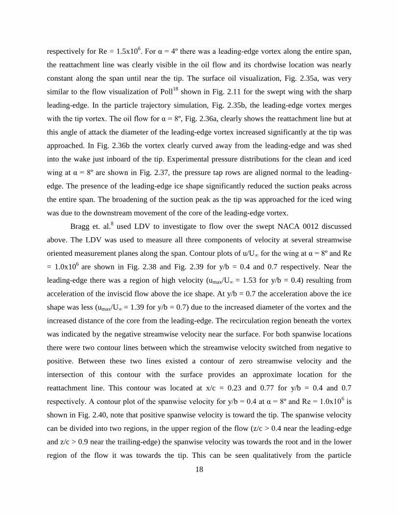
18

respectively for Re = 1.5x106. For α = 4º there was a leading-edge vortex along the entire span,

the reattachment line was clearly visible in the oil flow and its chordwise location was nearly

constant along the span until near the tip. The surface oil visualization, Fig. 2.35a, was very

similar to the flow visualization of Poll18

shown in Fig. 2.11 for the swept wing with the sharp

leading-edge. In the particle trajectory simulation, Fig. 2.35b, the leading-edge vortex merges

with the tip vortex. The oil flow for α = 8º, Fig. 2.36a, clearly shows the reattachment line but at

this angle of attack the diameter of the leading-edge vortex increased significantly at the tip was

approached. In Fig. 2.36b the vortex clearly curved away from the leading-edge and was shed

into the wake just inboard of the tip. Experimental pressure distributions for the clean and iced

wing at α = 8º are shown in Fig. 2.37, the pressure tap rows are aligned normal to the leading-

edge. The presence of the leading-edge ice shape significantly reduced the suction peaks across

the entire span. The broadening of the suction peak as the tip was approached for the iced wing

was due to the downstream movement of the core of the leading-edge vortex.

Bragg et. al.8 used LDV to investigate to flow over the swept NACA 0012 discussed

above. The LDV was used to measure all three components of velocity at several streamwise

oriented measurement planes along the span. Contour plots of u/U∞ for the wing at α = 8º and Re

= 1.0x106

are shown in Fig. 2.38 and Fig. 2.39 for y/b = 0.4 and 0.7 respectively. Near the

leading-edge there was a region of high velocity (umax/U∞ = 1.53 for y/b = 0.4) resulting from

acceleration of the inviscid flow above the ice shape. At y/b = 0.7 the acceleration above the ice

shape was less (umax/U∞ = 1.39 for y/b = 0.7) due to the increased diameter of the vortex and the

increased distance of the core from the leading-edge. The recirculation region beneath the vortex

was indicated by the negative streamwise velocity near the surface. For both spanwise locations

there were two contour lines between which the streamwise velocity switched from negative to

positive. Between these two lines existed a contour of zero streamwise velocity and the

intersection of this contour with the surface provides an approximate location for the

reattachment line. This contour was located at x/c = 0.23 and 0.77 for y/b = 0.4 and 0.7

respectively. A contour plot of the spanwise velocity for y/b = 0.4 at α = 8º and Re = 1.0x106 is

shown in Fig. 2.40, note that positive spanwise velocity is toward the tip. The spanwise velocity

can be divided into two regions, in the upper region of the flow (z/c > 0.4 near the leading-edge

and z/c > 0.9 near the trailing-edge) the spanwise velocity was towards the root and in the lower

region of the flow it was towards the tip. This can be seen qualitatively from the particle

19

trajectory simulation shown in Fig. 2.36b. The initial direction of the flow in the separated shear

layer was approximately normal to the leading-edge, the spanwise velocity was therefore

negative, and then the flow rolled over to form the vortex with a spanwise velocity towards the

tip. The magnitude of the spanwise velocity was significant, reaching v/U∞ = 0.57 near the

surface for y/b = 0.4. The largest spanwise velocity measured was v/U∞ = -0.62 and occurred at

y/b = 0.85, this large velocity towards the root was attributed in part to the tip vortex.

This review has provided a general overview of swept wing aerodynamics and the effects

of ice accretions on the performance and flowfield of swept wings. The results of previous swept

wing icing studies demonstrate the complex influence the ice can have. While the data presented

above is very insightful there are several areas in which knowledge is lacking. There is currently

no aerodynamic performance data high Reynolds number and the few flowfields studies that

have been conducted have used very simple swept wing geometries.

20

2.4 Figures

Fig. 2.1 Diagram of swept wing.

Fig. 2.2 Lift coefficient distribution of a straight wing.

Adapted from Katz.10

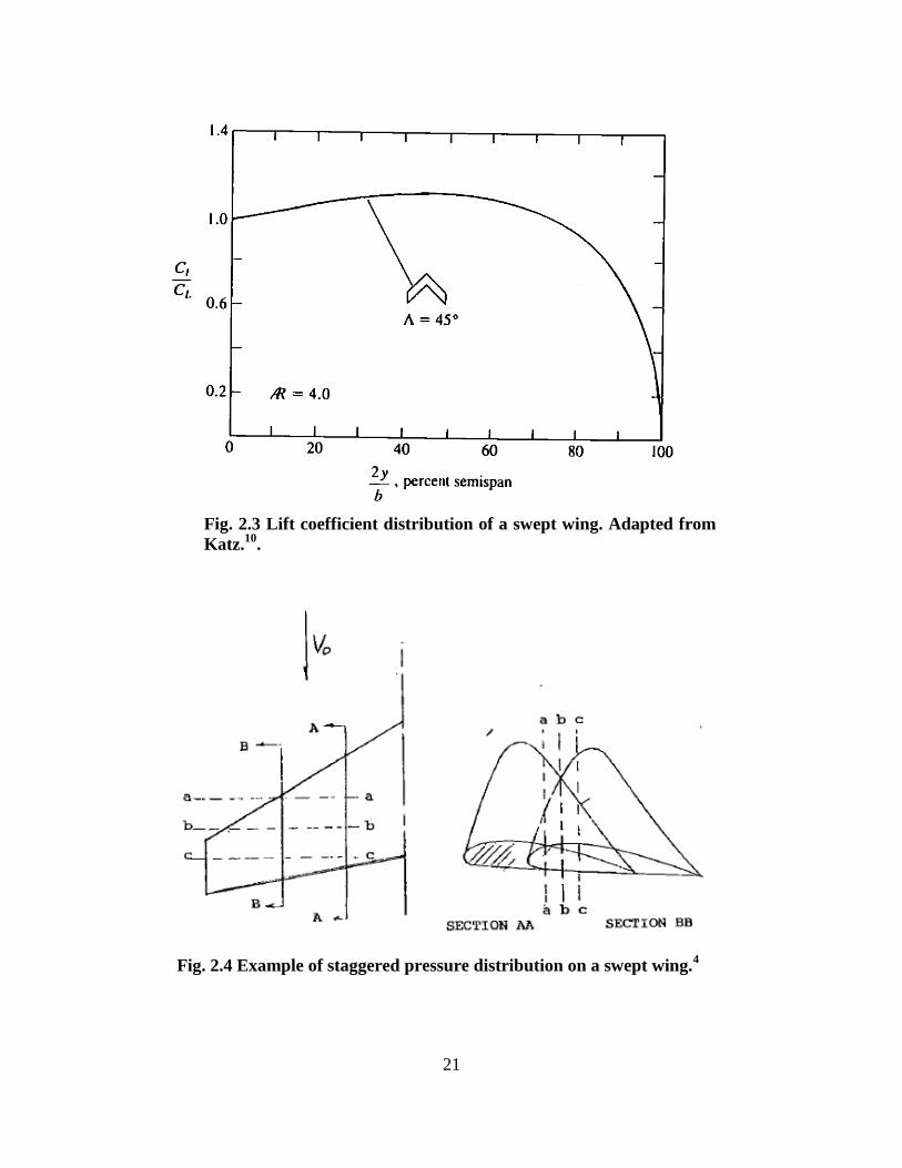
21

Fig. 2.4 Example of staggered pressure distribution on a swept wing.4

Fig. 2.3 Lift coefficient distribution of a swept wing. Adapted from

Katz.10

.

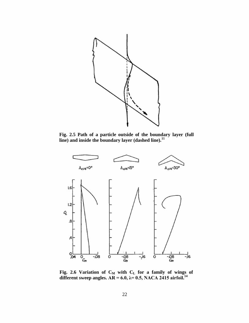
22

Fig. 2.5 Path of a particle outside of the boundary layer (full

line) and inside the boundary layer (dashed line).11

Fig. 2.6 Variation of CM with CL for a family of wings of

different sweep angles. AR = 6.0, λ= 0.5, NACA 2415 airfoil.14

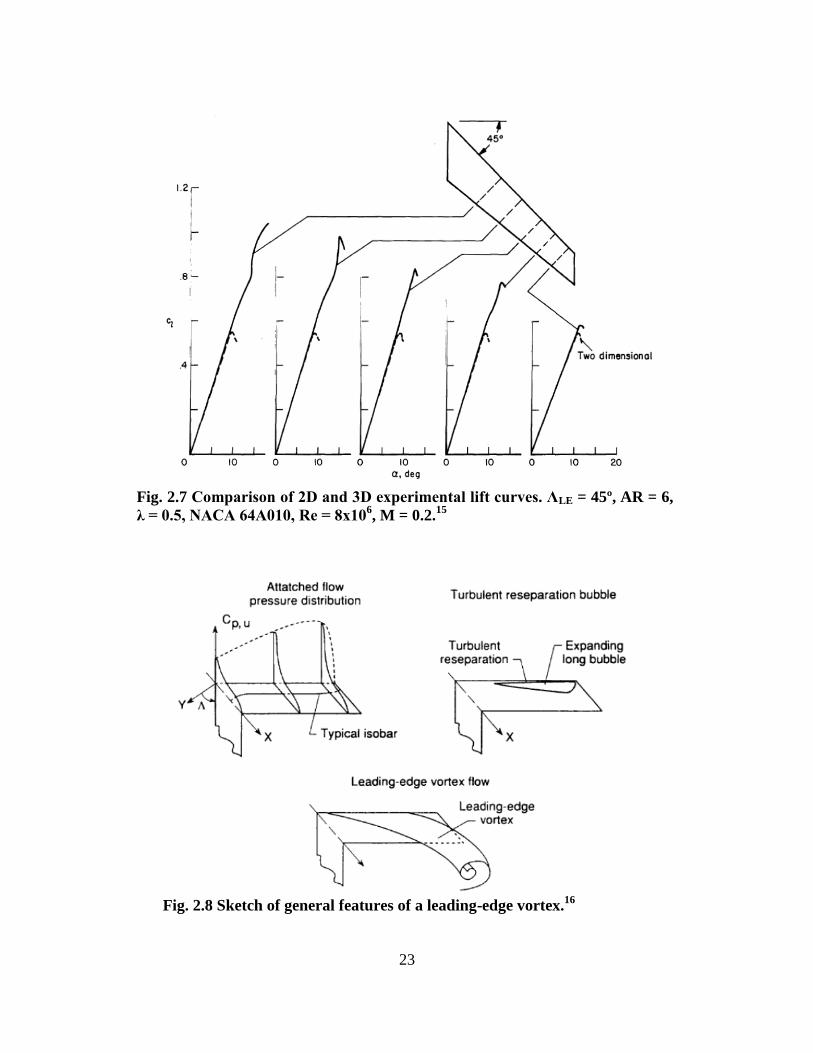
23

Fig. 2.7 Comparison of 2D and 3D experimental lift curves. ΛLE = 45º, AR = 6,

λ = 0.5, NACA 64A010, Re = 8x106, M = 0.2.

15

Fig. 2.8 Sketch of general features of a leading-edge vortex.16

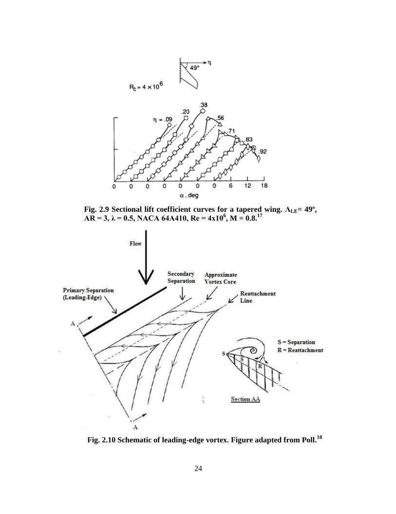
24

Fig. 2.9 Sectional lift coefficient curves for a tapered wing. ΛLE= 49º,

AR = 3, λ = 0.5, NACA 64A410, Re = 4x106, M = 0.8.

17

Fig. 2.10 Schematic of leading-edge vortex. Figure adapted from Poll.18

25

Fig. 2.11 Surface oil flow pattern showing spanwise running separation

bubble. α = 7º, ΛLE= 30º, r/c = 0.0003 and Re = 1.7x106.18

Fig. 2.12 Surface oil flow pattern showing a burst vortex. α = 10º,

ΛLE= 30º, r/c = 0.0003 and Re = 1.7x106.18

26

Fig. 2.13 Surface oil flow and pressure distributions for a full-span

leading-edge vortex. α = 11º, ΛLE= 56º, r/c = 0.0003 and Re = 2.7x106.18

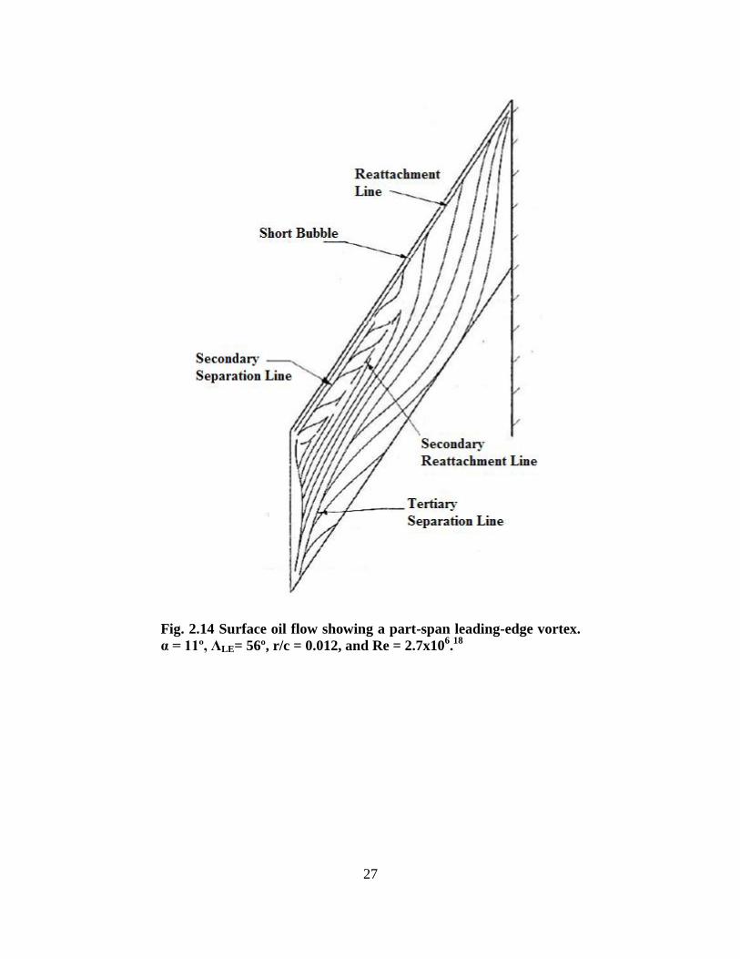
27

Fig. 2.14 Surface oil flow showing a part-span leading-edge vortex.

α = 11º, ΛLE= 56º, r/c = 0.012, and Re = 2.7x106.18

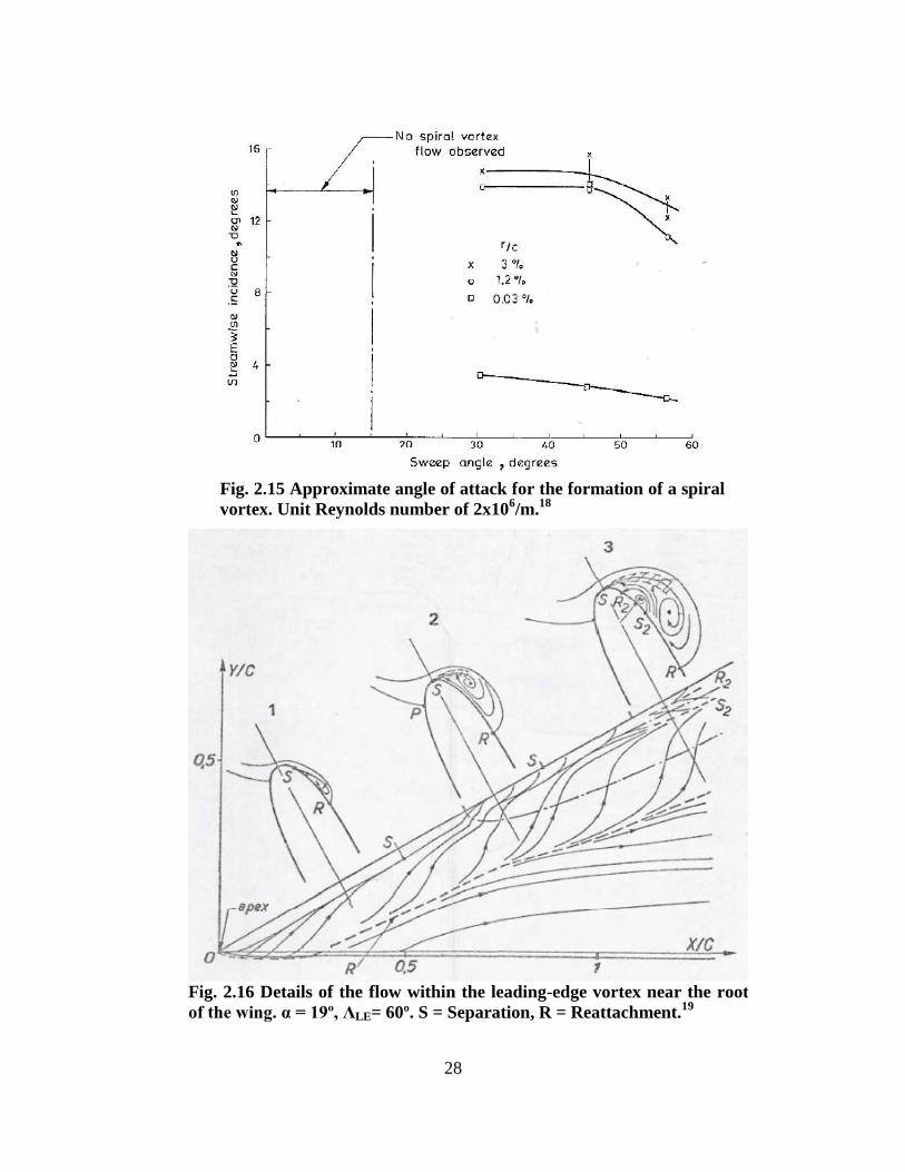
28

Fig. 2.15 Approximate angle of attack for the formation of a spiral

vortex. Unit Reynolds number of 2x106/m.

18

Fig. 2.16 Details of the flow within the leading-edge vortex near the root

of the wing. α = 19º, ΛLE= 60º. S = Separation, R = Reattachment.19

29

Fig. 2.17 Oil flow Reynolds number comparison. α = 15º, ΛLE= 30º and r/c =

0.03. a) Re = 0.9x106, b) 1.7x10

6.18

Fig. 2.18 Effect of Reynolds number on the lift of a swept wing with ΛLE=

50º.16

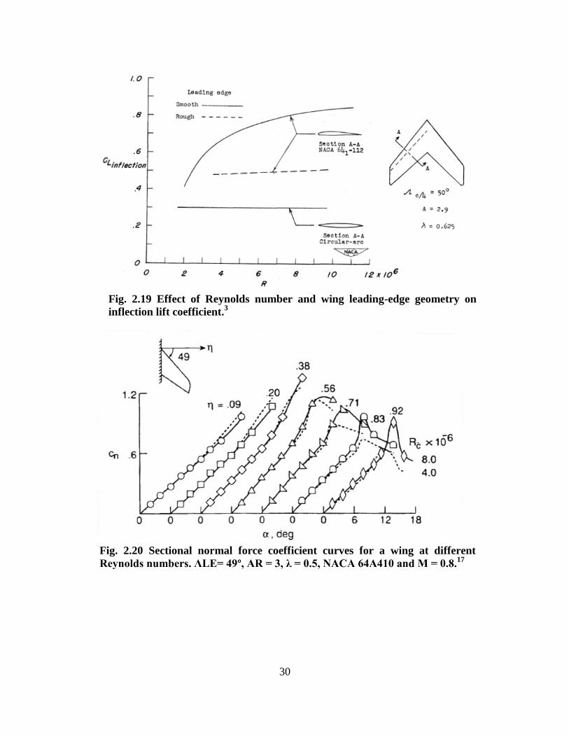
30

Fig. 2.19 Effect of Reynolds number and wing leading-edge geometry on

inflection lift coefficient.3

Fig. 2.20 Sectional normal force coefficient curves for a wing at different

Reynolds numbers. ΛLE= 49º, AR = 3, λ = 0.5, NACA 64A410 and M = 0.8.17

31

Fig. 2.21 Section normal force coefficients for a wing at two different Reynolds

numbers. Λc/4= 35º, AR = 5, λ = 0.7, NACA 651A012 (streamwise) and M = 0.25.22

Fig. 2.22 Section normal force coefficients for a wing at two different Reynolds

numbers. Λc/4= 35º, AR = 5, λ = 0.7, NACA 651A012 (streamwise) and M = 0.8.22

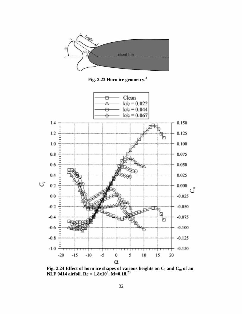
32

Fig. 2.23 Horn ice geometry.2

Fig. 2.24 Effect of horn ice shapes of various heights on Cl and Cm of an

NLF 0414 airfoil. Re = 1.8x106, M=0.18.

23

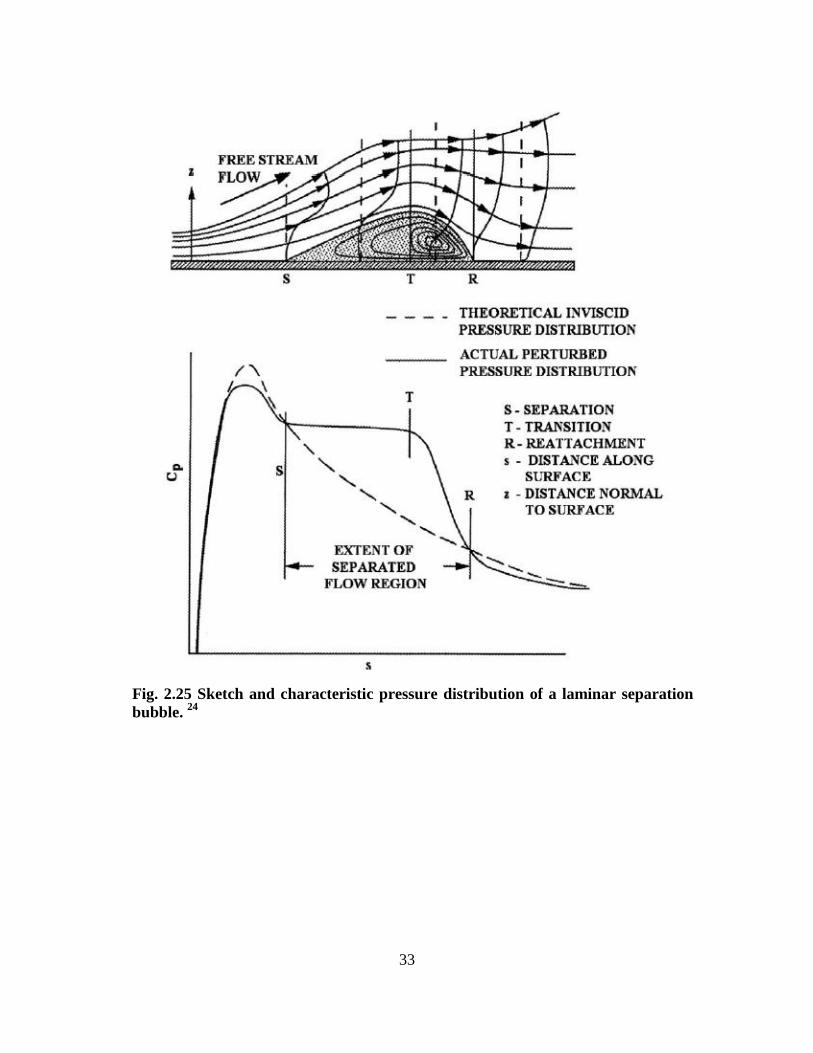
33

Fig. 2.25 Sketch and characteristic pressure distribution of a laminar separation

bubble. 24

34

Fig. 2.26 Comparison of pressure distribution for a NACA 0012 with and

without a simulated horn ice shape, α = 4º, Re = 1.5x106 and M = 0.12.

25

Fig. 2.27 Separation streamlines behind a simulated horn ice shape for

various angles of attack, Re = 1.5x106 and M = 0.12.

25

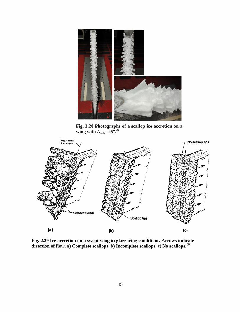
35

Fig. 2.28 Photographs of a scallop ice accretion on a

wing with ΛLE= 45º.26

Fig. 2.29 Ice accretion on a swept wing in glaze icing conditions. Arrows indicate

direction of flow. a) Complete scallops, b) Incomplete scallops, c) No scallops.26

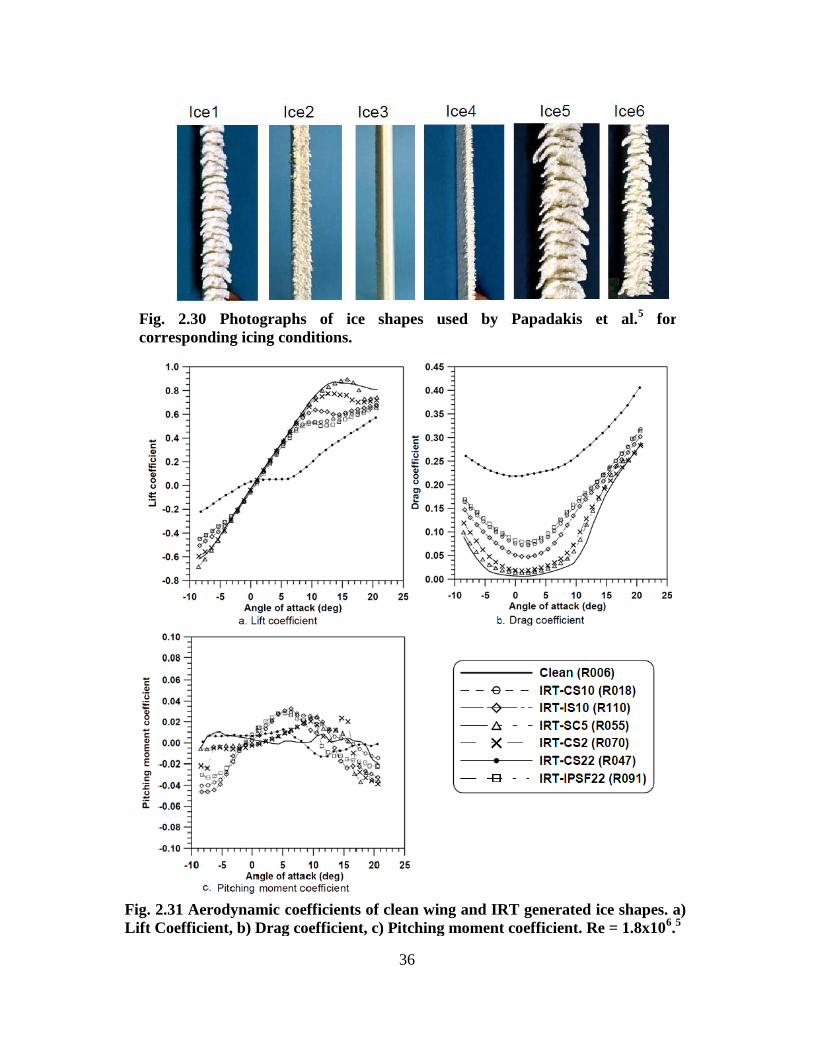
36

Fig. 2.30 Photographs of ice shapes used by Papadakis et al.5 for

corresponding icing conditions.

Fig. 2.31 Aerodynamic coefficients of clean wing and IRT generated ice shapes. a)

Lift Coefficient, b) Drag coefficient, c) Pitching moment coefficient. Re = 1.8x106.5

37

Fig. 2.32 Ice shape simulations for 25% scale T-Tail model.29

Fig. 2.33 Effect of horn ice simulations on CL of the 25% T-

Tail model at Re = 1.36x106

.29

38

Fig. 2.34 Cross-section of the ice shape simulation

used by Bragg et. al.7,8

on a swept NACA 0012.

Fig. 2.35 CFD results for swept wing with leading-edge ice accretion.30

a) Surface oil

flow simulation, b) Particle trajectory simulation. α = 4º, Re = 1.5x106.

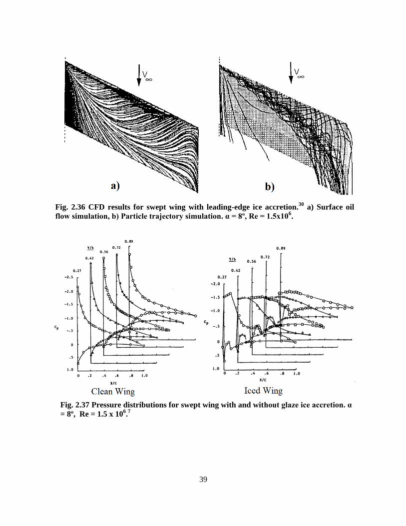
39

Fig. 2.36 CFD results for swept wing with leading-edge ice accretion.30

a) Surface oil

flow simulation, b) Particle trajectory simulation. α = 8º, Re = 1.5x106.

Fig. 2.37 Pressure distributions for swept wing with and without glaze ice accretion. α

= 8º, Re = 1.5 x 106.7

40

Fig. 2.38 (u/U∞) velocity contours on wing upper surface at y/b = 0.4. α = 8º, Re

= 1.0x106.8

Fig. 2.39 (u/U∞) velocity contours on wing upper surface at y/b = 0.70. α = 8º,

Re = 1.0x106.8

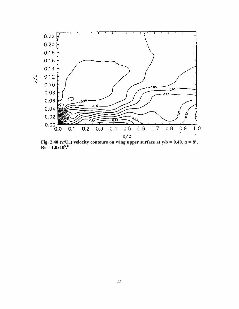
41

Fig. 2.40 (v/U∞) velocity contours on wing upper surface at y/b = 0.40. α = 8º,

Re = 1.0x106.8

42

Chapter 3

Experimental Methods

This chapter will describe the facility, equipment and the various experimental methods

used in this work. Included are descriptions of the wind tunnel, force balance, pressure

measurement system and the swept wing model. The wind tunnel wall corrections will also be

described. The experimental methods include the basic aerodynamic performance measurements,

surface pressure measurements, surface oil flow visualization and a five-hole probe wake survey.

3.1 Aerodynamic Testing

3.1.1 Wind Tunnel

The aerodynamic testing for this project was performed in the University of Illinois

subsonic wind tunnel. The wind tunnel is of the open-return type with a rectangular test section

measuring 2.8-ft by 4-ft. The contraction ratio between the inlet and test section was 7.5:1. To

reduce turbulence in the test section the inlet settling section contained a four-inch thick

honeycomb section followed by four anti-turbulence screens, this effectively reduced the

turbulence intensity to less than 0.1% over the full range of operating speeds. In order to reduce

the streamwise pressure gradient resulting from tunnel wall boundary-layer growth the

downstream end of the test section was 0.5 inches wider than the upstream end. An illustration of

the tunnel is shown in Fig. 3.1.

The tunnel was powered by a 125-hp AC motor regulated by an ABB ACS 600 Low

Voltage AC Drive. The motor was used to drive a 5 bladed fan up to a maximum of 1200 rpm.

The maximum speed in the empty test section was approximately 165 mph (242 ft/s). The

Reynolds number of the swept wing model was calculated using the tunnel freestream velocity

and the mean aerodynamic chord measured in the streamwise direction.

(3.1)

During operation, the Reynolds number was held to within 0.5%. The velocity in the test

section was calculated using the difference between the static pressure in the settling section ( )

and the static pressure in the test section ( ). The pressure difference was measured using a

43

Setra 239 differential pressure transducer. A pressure tap was located on each of the four walls of

the settling section, and another set of four taps were located on the walls just upstream of the

test section. Each set of 4 taps were pneumatically averaged and then connected to the Setra 239.

The velocity was calculated by first using Bernoulli’s equation to relate the total pressure in the

settling section and the test section, and then mass conservation was applied to solve for the

velocity in the test section.

(3.2)

(3.3)

√ ( )

(

) (3.5)

The ideal gas law was used to calculate the ambient density .

(3.6)

Where R is the ideal gas constant for air and and where the ambient pressure and

temperature respectively. The ambient pressure was measured using a Setra 270 pressure

transducer located in the control room and the temperature was measured using an Omega

Thermocouple located near the wind tunnel.

3.1.2 Swept Wing Model

A semispan swept wing model was designed and built for this investigation. It was

desired to use an existing realistic swept wing typical of modern commercial airliners and for

this reason the wing of the Common Research Model (CRM) was chosen. The CRM was

designed by Vassberg et. al.31

for the 4th

AIAA Drag Prediction Workshop, a 3D model of the

CRM is shown in Fig. 3.2. The CRM was designed to represent a typical wide body swept wing

commercial airliner with a modern transonic airfoil. The CRM was chosen because the geometry

as well as experimental and computational data are publicly available. The original CRM has an

aspect ratio of 9, LE sweep of 35 deg., a taper ratio of 0.275 and 8 degrees of twist from the root

44

to the tip. Several modifications were made for the UIUC model to ease construction and reduce

cost. These modifications included the removal of dihedral, linearizing the twist distribution and

increasing the airfoil thickness by 20% around the mean camber line. The important geometric

features of the CRM and the UIUC model are summarized in Table 3.1. On the original CRM

the first 10% of the span is located within the fuselage of the aircraft and this area was not used

for the UIUC model resulting in a change in aspect ratio and taper ratio.

Table 3.1 Geometric Comparison of CRM and UIUC Wind Tunnel Model

Illinois Model CRM

AR 8.3 9.0

LE Sweep 35 35

cmac (ft) 0.5167 11.98

Max Thickness (ft) 0.1458 4

Min Thickness (ft) 0.0241 0.85

Semispan b/2 (ft) 2.1 96.4

Taper Ratio 0.296 0.275

A steel frame, shown in Fig. 3.3, was fabricated for structural support. The frame

mounted directly to the force balance through the tunnel floor as shown in Fig. 3.3. The exterior

shell of the model was manufactured using the rapid-prototype process stereolithography (SLA).

This shell consisted of three components; a lower surface, upper surface and a leading-edge, all

shown in Fig. 3.4. A clean and an iced leading-edge were built and were designed to be easily

interchangeable during testing. Surface pressure taps were formed during the SLA process, a row

of pressure taps on the upper surface can be seen in Fig. 3.5. The model contained a total of 116

pressure taps although not all were used as will be explained below.

The upper and lower surfaces were made up of a thin skin and structural ridges for

support, Fig. 3.6. The model was designed so that the upper and lower surface components fit

over the steel frame and bolted directly to each other. The bolts passed through the lower surface

into a threaded insert located in the structural ridges of the upper surface component, see Fig.

3.7. Fig. 3.8 shows several important features of the steel frame including leading-edge tabs and

grooves for pressure lines. The removable leading-edge bolted directly onto the leading-edge

tabs on the steel frame, as shown in Fig. 3.9. This made it a simple process to remove the

leading-edge while keeping the upper and lower surfaces in place.

Unfortunately, because the SLA shell was so thin the model warped in several areas. As a

result, the seam where the removable leading-edge met the upper surface could not be held to the

45

desired tolerances. There were small gaps between the two surfaces and in some areas the upper

surface was higher than the leading-edge surface resulting in a step. Fortunately, the goal of this

research was not to assess the aerodynamics of this particular wing, but rather investigate the use

of various methods that can be used to assess the aerodynamics of a wing with a leading-edge ice

accretion. It was therefore decided that the surface imperfections were of secondary importance.

To minimize the effect of these imperfections modeling clay was used to smooth the surface

imperfections. A redesigning of the wing to eliminate these problems is underway but was not

completed in time for this research.

As mentioned above the model contained 116 pressure taps, these pressure taps were

organized into 5 streamwise oriented rows. The spanwise location of each row of taps and the

number of taps in each row are shown in Table 3.2.

Table 3.2 Spanwise location of each tap row

and the number of pressure taps.

Row 2y/b Number of Taps

1 0.11 30

2 0.36 27

3 0.55 24

4 0.77 20

5 0.92 15

Before testing it was necessary to connect tubing to the pressure taps and then run this

tubing out of the model. Each pressure line consisted of a small length of 0.042-in. hypodermic

steel tubing inserted into the tap. Then 0.043-in. diameter vinyl tubing was connected to the steel

tubing and run throughout the model. The procedure for connecting a pressure line to a tap was

as follows:

1. Cut a small length of steel tubing, typically 1-2 inches.

2. Apply heat to the steel tubing, using a blow torch, so that the tube becomes soft

enough to easily bend.

3. Connect the necessary length of plastic tubing to the steel tubing.

4. Insert the steel tubing into the pressure tap, ensuring that the end is flush with the

upper surface.

5. Using epoxy, glue the tubing into place.

46

Several tubes connected to the leading and trailing-edge taps had to first pass over the steel frame

to get to the interior of the model where they were then run out the bottom of the model. The

purpose of the grooves in the steel frame, shown in Fig. 3.8, was to allow these pressure lines to

pass over the frame. Unfortunately, due to space constraints several of the pressure taps were not

connected. Most of the missing taps were in the last row (2y/b = 0.92) where only 9 of the 15

taps were connected. No taps in the leading or trailing edge of the 5th

row were connected. In

addition there were a few taps throughout the model that could not be used because they became

blocked during installation.

3.1.3 Data Acquisition

The data acquisition system for this research was controlled from a Dell Precision T3400

computer with an Intel CoreTM

Quad CPU with 4GB RAM. A Windows XP 32-bit operating

system was used. All software was written in-house using LabVIEW 2010. The software sent

commands to the various equipment including the force balance, tunnel variable frequency drive,

wake rake traverse and pressure measuring system. Analog signals were digitized using a

National Instruments 16 bit A/D conversion board.

3.1.3.1 Force Balance Measurements

As mentioned above, the steel frame of the model was mounted directly to the force

balance through the floor of the tunnel. The balance, built by Aerotech ATE Limited, was used

to measure lift, drag and pitching moment about the quarter chord of the mean aerodynamic

chord; a photograph of the model attached to the balance is shown in Fig. 3.10. The turntable

was used to set the angle of attack within 0.1º. The balance used load cells to measure the normal

and axial force as well as the pitching moment about the center of the balance. The force balance

contained its own signal conditioning system and could be set to measure loads in three different

ranges shown in Table 3.3.

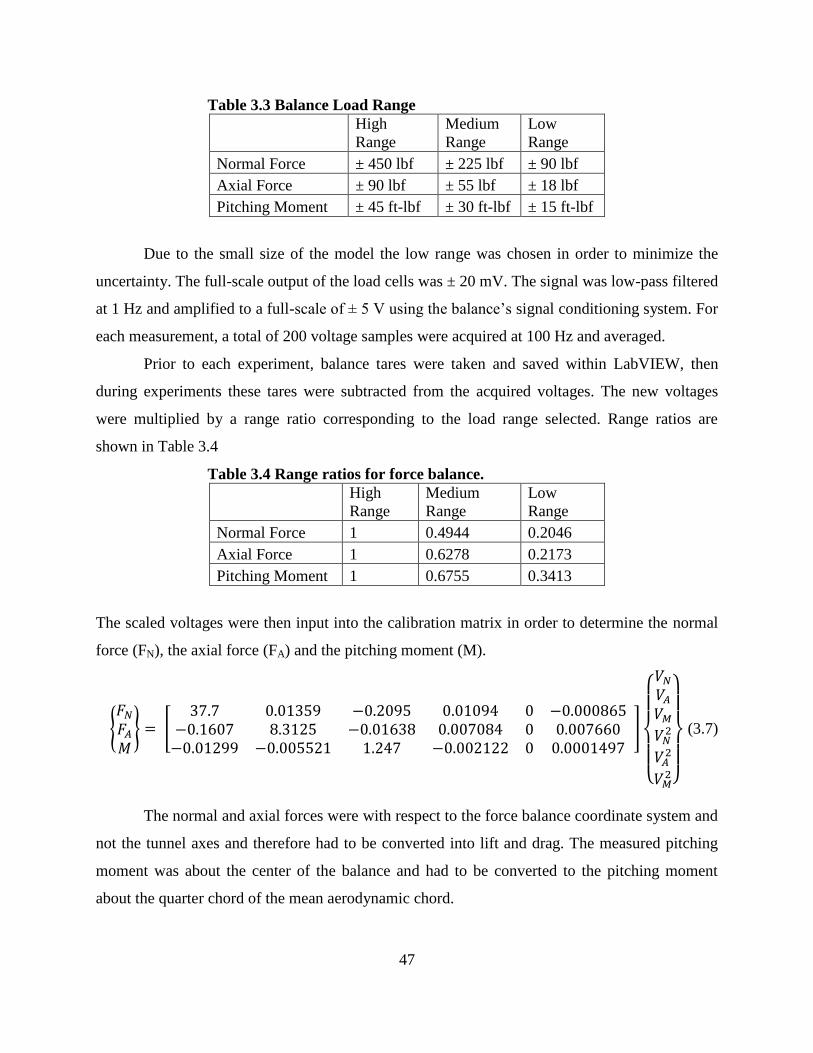
47

Table 3.3 Balance Load Range

High

Range

Medium

Range

Low

Range

Normal Force ± 450 lbf ± 225 lbf ± 90 lbf

Axial Force ± 90 lbf ± 55 lbf ± 18 lbf

Pitching Moment ± 45 ft-lbf ± 30 ft-lbf ± 15 ft-lbf

Due to the small size of the model the low range was chosen in order to minimize the

uncertainty. The full-scale output of the load cells was ± 20 mV. The signal was low-pass filtered

at 1 Hz and amplified to a full-scale of ± 5 V using the balance’s signal conditioning system. For

each measurement, a total of 200 voltage samples were acquired at 100 Hz and averaged.

Prior to each experiment, balance tares were taken and saved within LabVIEW, then

during experiments these tares were subtracted from the acquired voltages. The new voltages

were multiplied by a range ratio corresponding to the load range selected. Range ratios are

shown in Table 3.4

Table 3.4 Range ratios for force balance.

High

Range

Medium

Range

Low

Range

Normal Force 1 0.4944 0.2046

Axial Force 1 0.6278 0.2173

Pitching Moment 1 0.6755 0.3413

The scaled voltages were then input into the calibration matrix in order to determine the normal

force (FN), the axial force (FA) and the pitching moment (M).

{

} [

]

{

}

(3.7)

The normal and axial forces were with respect to the force balance coordinate system and

not the tunnel axes and therefore had to be converted into lift and drag. The measured pitching

moment was about the center of the balance and had to be converted to the pitching moment

about the quarter chord of the mean aerodynamic chord.

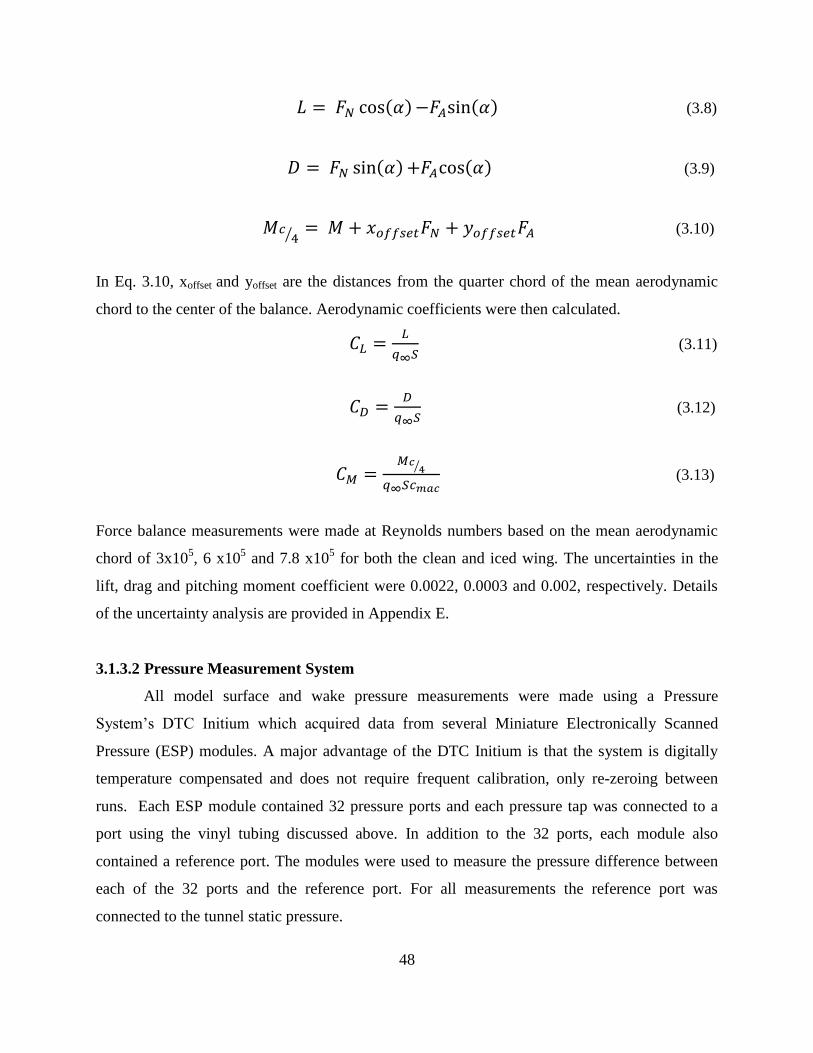
48

( ) ( ) (3.8)

( ) ( ) (3.9)

⁄

(3.10)

In Eq. 3.10, xoffset and yoffset are the distances from the quarter chord of the mean aerodynamic

chord to the center of the balance. Aerodynamic coefficients were then calculated.

(3.11)

(3.12)

⁄

(3.13)

Force balance measurements were made at Reynolds numbers based on the mean aerodynamic

chord of 3x105, 6 x10

5 and 7.8 x10

5 for both the clean and iced wing. The uncertainties in the

lift, drag and pitching moment coefficient were 0.0022, 0.0003 and 0.002, respectively. Details

of the uncertainty analysis are provided in Appendix E.

3.1.3.2 Pressure Measurement System

All model surface and wake pressure measurements were made using a Pressure

System’s DTC Initium which acquired data from several Miniature Electronically Scanned

Pressure (ESP) modules. A major advantage of the DTC Initium is that the system is digitally

temperature compensated and does not require frequent calibration, only re-zeroing between

runs. Each ESP module contained 32 pressure ports and each pressure tap was connected to a

port using the vinyl tubing discussed above. In addition to the 32 ports, each module also

contained a reference port. The modules were used to measure the pressure difference between

each of the 32 ports and the reference port. For all measurements the reference port was

connected to the tunnel static pressure.

49

A schematic of the Initium setup is shown in Fig. 3.11, the units label DTC Scanner

represent digitally temperature compensated ESP modules. The Initium connected to the

computer via a 10/100 Base – T Ethernet cable and each ESP module connected to the Initium

via PSCB cables. The throughput rate of the system is 650 Hz/channel when scanning 32

channels per scanner. A supply of compressed nitrogen is connected to the Initium as shown in

Fig. 3.11. In order to re-zero each ESP module a manifold within the module is shifted, this is

accomplished by applying 100 psi of compressed nitrogen through the C1 line shown in Fig.

3.11. The manifold is then shifted back by applying 100 psi to the C2 line and the system is

ready for data acquisition.

A total of 5 ESP modules were used, one ± 5.0 psid module, two ± 1.0 psid modules and

two ± 0.35 psid modules. For measuring the static pressure on the model surface the ± 5.0 psid

module was used for many of the taps near the leading-edge where the pressure difference was

greatest. The remaining taps near the leading-edge were connected to the two ± 1.0 psid modules

and any remaining taps were connected to a ± 0.35 psid module. The second ± 0.35 psid module

was for the wake surveys.

3.1.4 Wake Survey System

Wake surveys are typically used when testing 2D airfoils in order to obtain an accurate

sectional drag coefficient. A two-dimensional wake survey requires measurements of total

pressure in the wake of the body and then through a control volume analysis the drag can be

calculated. In three dimensions the wake survey is more difficult, but can provide more

information. By measuring the total and static pressure as well as all three components of

velocity in the wake it is possible to calculate the lift and drag of the body and decompose the

drag into profile and induced drag.32,33

In addition, the spanwise distribution of lift and drag can

be calculated. These results can provide a valuable diagnostic tool for a wing making the wake

survey an important aspect of this work. In order to obtain measurements of total and static

pressure, as well as the three components of velocity, a five-hole probe (5HP) was utilized.

The probe used in this study was an Aeroprobe Corp., model PS5-C318-152 five-hole

probe. The probe tip was conical with a base diameter of 0.125-in. On the probe tip were five

pressure ports, a central port at the tip of the cone and four evenly spaced peripheral ports. Each

port was connected to an individual pressure line that was then connected to one of the ports of

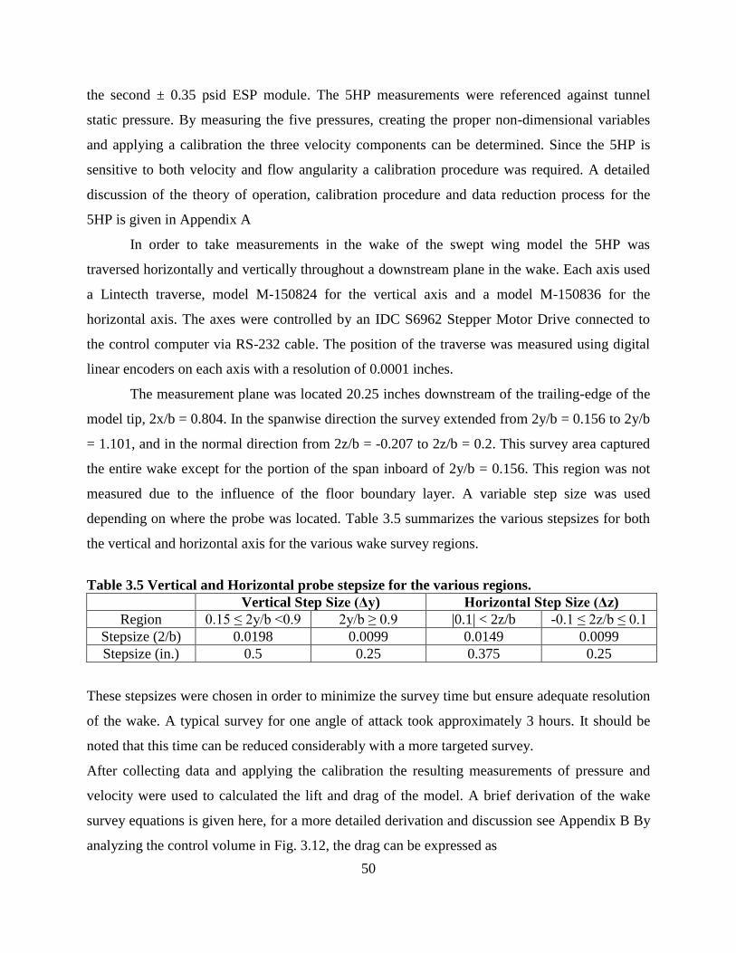
50

the second ± 0.35 psid ESP module. The 5HP measurements were referenced against tunnel

static pressure. By measuring the five pressures, creating the proper non-dimensional variables

and applying a calibration the three velocity components can be determined. Since the 5HP is

sensitive to both velocity and flow angularity a calibration procedure was required. A detailed

discussion of the theory of operation, calibration procedure and data reduction process for the

5HP is given in Appendix A

In order to take measurements in the wake of the swept wing model the 5HP was

traversed horizontally and vertically throughout a downstream plane in the wake. Each axis used

a Lintecth traverse, model M-150824 for the vertical axis and a model M-150836 for the

horizontal axis. The axes were controlled by an IDC S6962 Stepper Motor Drive connected to

the control computer via RS-232 cable. The position of the traverse was measured using digital

linear encoders on each axis with a resolution of 0.0001 inches.

The measurement plane was located 20.25 inches downstream of the trailing-edge of the

model tip, 2x/b = 0.804. In the spanwise direction the survey extended from 2y/b = 0.156 to 2y/b

= 1.101, and in the normal direction from 2z/b = -0.207 to 2z/b = 0.2. This survey area captured

the entire wake except for the portion of the span inboard of 2y/b = 0.156. This region was not

measured due to the influence of the floor boundary layer. A variable step size was used

depending on where the probe was located. Table 3.5 summarizes the various stepsizes for both

the vertical and horizontal axis for the various wake survey regions.

Table 3.5 Vertical and Horizontal probe stepsize for the various regions.

Vertical Step Size (Δy) Horizontal Step Size (Δz)

Region 0.15 ≤ 2y/b <0.9 2y/b ≥ 0.9 |0.1| < 2z/b -0.1 ≤ 2z/b ≤ 0.1

Stepsize (2/b) 0.0198 0.0099 0.0149 0.0099

Stepsize (in.) 0.5 0.25 0.375 0.25

These stepsizes were chosen in order to minimize the survey time but ensure adequate resolution

of the wake. A typical survey for one angle of attack took approximately 3 hours. It should be

noted that this time can be reduced considerably with a more targeted survey.

After collecting data and applying the calibration the resulting measurements of pressure and

velocity were used to calculated the lift and drag of the model. A brief derivation of the wake

survey equations is given here, for a more detailed derivation and discussion see Appendix B By

analyzing the control volume in Fig. 3.12, the drag can be expressed as

51

∬ ( )

∬ (

)

(3.14)

Where , and represent the three components of velocity in the wake. Notice the first

integral is only over the viscous wake region ( ) because outside of the wake. The

second term however requires measurements over the entire downstream plane S2. This is

impractical in most wind tunnel facilities and therefore it is necessary to develop an expression

for the drag that only requires measurements in the viscous wake. Following the method of

Betz34

it can be shown, see Appendix B that Eq. 3.14 can be separated into an expression for

profile drag ( ) and an expression for induced drag ( ).

∬ (( ) ( )( ( ))) (3.15)

∬ ( )

(3.16)

In Eq. 3.15 the terms and are known as the artificial velocity and the blockage correction

term respectively, see Appendix B for the definitions of these terms. The profile drag given by

Eq. 3.15 only requires measurements of total pressure and streamwise velocity within the wake

region; however, the induced drag given by Eq. 3.16 still requires measurements over the entire

downstream plane S2. Maskell35

solved this problem by deriving the following result, details in

Appendix B

∬ ( )

(3.17)

The terms and represent the streamwise vorticity and the transverse source term respectively.

(3.18)

(3.19)

The terms and represent the stream function and velocity potential in the transverse plane

respectively. The vorticity and source term can be determined directly from differentiating the

transverse velocity components and then the stream function and velocity potential can be

calculated by solving the following Poisson equations.

(3.20)

52

(3.21)

Equations 3.20 and 3.21 must be solved over the entire downstream plane S2, but outside of the

wake the vorticity and source term are zero so the Poisson equations reduce to Laplace’s

equation and therefore measurements are only required within the wake. In many cases the term

in Eq. 3.17 is small and therefore negligible.32

For this study, this term was dropped and

induced drag was calculated using Eq. 3.22.

∬

(3.22)

Using Eqs. 3.15 and 3.22 the profile and induced drag can be determined separately and the total

drag is given by the sum of these two components. Integrating Eqs. 3.15 and 3.22 in the z-

direction gives the spanwise distribution of the profile and induced drag.

Maskell35

also derived an expression for the lift that only requires measurements in the

wake region.

∬

(3.23)

The sectional lift coefficient can be derived using classical wing theory.33

( ) ( ) (3.24)

Where ( ) and ( ) represent the chord distribution and the circulation distribution

respectively. The circulation distribution is determined by integrating the streamwise vorticity.

The methods applied in solving the various equations related to the wake surveys are discussed

in Appendix C.

3.1.5 Tunnel Corrections

Due to the proximity of the tunnel walls the flow around the model and the resulting

forces will be different relative to the free-air case. The influence of the tunnel walls is generally

assumed to be due to several independent mechanisms whose effects are additive.36

The primary

effects that require corrections are horizontal buoyancy, solid blockage, wake blockage,

streamline curvature and boundary induced upwash. Horizontal buoyancy refers to a streamwise

static pressure gradient resulting from the wall boundary layer growth. As discussed in Section

3.1.1 the downstream end of the test section is 0.5 inches wider than the upstream end and

53

therefore the effects of buoyancy are considered negligible. The remaining effects will now be

discussed. All corrections were applied automatically by the LabVIEW code during data

acquisition.

3.1.5.1 Solid Blockage

By placing a solid body in the tunnel test section the effective area through which the air

can flow is reduced. By continuity this reduction in area results in an increase in velocity near the

model or equivalently an increase in the dynamic pressure felt by the model. An increase in the

dynamic pressure results in an increased forces and moments experience by the model. It is

generally assumed that increase in dynamic pressure is constant along the entire model and

therefore only a single correction applied to the freestream dynamic pressure is required.36

This

correction takes the form of a velocity increment. For this study Thom’s short-form equation for

solid blockage was used.37

( )

⁄ (3.25)

Where = 0.9 for a three dimensional wing and is the tunnel cross-section area. A

potentially more accurate expression for is discussed in Pope36

where . is a

function of airfoil type and thickness ratio and is a function of the tunnel aspect ratio and the

model span. Equation 3.25 was used in this study because the product is generally within 1-

2 percent of 0.9 and Eq. 3.25 does not require the airfoil type to be specified. For the model used

in this study = 0.001333.

3.1.5.2 Wake Blockage

The wake blockage correction used in this study is based on the work of Maskell38

and is

discussed in Pope.36

Maskell stated three important observations regarding wake blockage. First,

similar to solid blockage it was observed that wake blockage results in a higher dynamic pressure

felt by the model and that this increase in is constant along the entire model. Second, nearly

all 3D models require the same correction. Finally, the wake induces a pressure gradient on the

model which results in a drag increment similar to horizontal buoyancy. For a streamlined body

with no separated flow the wake blockage velocity increment is given by Eq. 3.26.

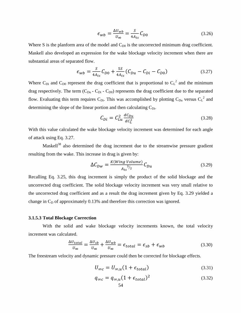
54

(3.26)

Where S is the planform area of the model and CD0 is the uncorrected minimum drag coefficient.

Maskell also developed an expression for the wake blockage velocity increment when there are

substantial areas of separated flow.

( ) (3.27)

Where CDi and CD0 represent the drag coefficient that is proportional to CL2 and the minimum

drag respectively. The term (CDu - CDi - CD0) represents the drag coefficient due to the separated

flow. Evaluating this term requires CDi. This was accomplished by plotting CDu versus CL2 and

determining the slope of the linear portion and then calculating CDi.

(3.28)

With this value calculated the wake blockage velocity increment was determined for each angle

of attack using Eq. 3.27.

Maskell38

also determined the drag increment due to the streamwise pressure gradient

resulting from the wake. This increase in drag is given by:

( )

⁄ (3.29)

Recalling Eq. 3.25, this drag increment is simply the product of the solid blockage and the

uncorrected drag coefficient. The solid blockage velocity increment was very small relative to

the uncorrected drag coefficient and as a result the drag increment given by Eq. 3.29 yielded a

change in CD of approximately 0.13% and therefore this correction was ignored.

3.1.5.3 Total Blockage Correction

With the solid and wake blockage velocity increments known, the total velocity

increment was calculated.

(3.30)

The freestream velocity and dynamic pressure could then be corrected for blockage effects.

( ) (3.31)

( ) (3.32)

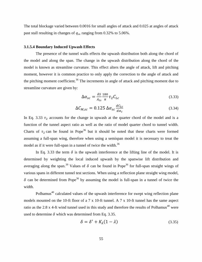
55

The total blockage varied between 0.0016 for small angles of attack and 0.025 at angles of attack

past stall resulting in changes of ranging from 0.32% to 5.06%.

3.1.5.4 Boundary Induced Upwash Effects

The presence of the tunnel walls effects the upwash distribution both along the chord of

the model and along the span. The change in the upwash distribution along the chord of the

model is known as streamline curvature. This effect alters the angle of attack, lift and pitching

moment, however it is common practice to only apply the correction to the angle of attack and

the pitching moment coefficient.36

The increments in angle of attack and pitching moment due to

streamline curvature are given by:

(3.33)

(3.34)

In Eq. 3.33 accounts for the change in upwash at the quarter chord of the model and is a

function of the tunnel aspect ratio as well as the ratio of model quarter chord to tunnel width.

Charts of can be found in Pope36

but it should be noted that these charts were formed

assuming a full-span wing, therefore when using a semispan model it is necessary to treat the

model as if it were full-span in a tunnel of twice the width.36

In Eq. 3.33 the term is the upwash interference at the lifting line of the model. It is

determined by weighting the local induced upwash by the spanwise lift distribution and

averaging along the span.39

Values of can be found in Pope36

for full-span straight wings of

various spans in different tunnel test sections. When using a reflection plane straight wing model,

can be determined from Pope36

by assuming the model is full-span in a tunnel of twice the

width.

Polhamus40

calculated values of the upwash interference for swept wing reflection plane

models mounted on the 10-ft floor of a 7 x 10-ft tunnel. A 7 x 10-ft tunnel has the same aspect

ratio as the 2.8 x 4-ft wind tunnel used in this study and therefore the results of Polhamus40

were

used to determine which was determined from Eq. 3.35.

( ) (3.35)

56

Where was the upwash interference assuming a wing with no taper and was a taper

correction factor. Both and were functions of the ratio of semispan to tunnel width and

sweep angle, and they were determined from a chart in Polhamus.40

Note that since these

correction factors were determined for a semispan wing it was not necessary to assume a full-

span wing. With the value of the upwash interference parameter known the final corrections

are applied to the drag and angle of attack.

(3.36)

(3.37)

These corrections account for the upwash induced by the walls along the span of the wing. This

upwash offsets some of the downwash produced by the trailing vortices and as a result the angle

of attack and induced drag will be too small. 36

Equation 3.36 is therefore a correction to the

induced drag and will be used to correct the induced drag measured by the wake survey.

3.1.5.5 Final Corrections

Expressions for the corrected values of the angle of attack, lift coefficient, drag

coefficient, pitching moment coefficient and pressure coefficient are given here. The lift

coefficient and surface pressure coefficient are corrected by non-dimesionalizng using the

corrected dynamic pressure.

( ) (3.38)

( ) (3.39)

The angle of attack is corrected by adding the increments due to streamline curvature and

boundary induced upwash .

( ) (3.40)

The drag coefficient and pitching moment coefficient are then corrected by first non-

dimensionalizing by the corrected dynamic pressure and then adding the correction factors due to

boundary induced upwash and streamline curvature.

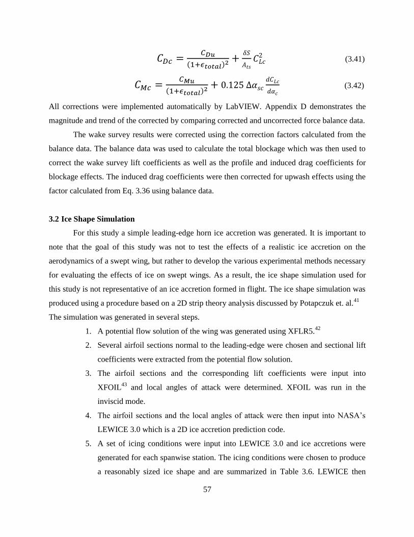
57

( )

(3.41)

( )

(3.42)

All corrections were implemented automatically by LabVIEW. Appendix D demonstrates the

magnitude and trend of the corrected by comparing corrected and uncorrected force balance data.

The wake survey results were corrected using the correction factors calculated from the

balance data. The balance data was used to calculate the total blockage which was then used to

correct the wake survey lift coefficients as well as the profile and induced drag coefficients for

blockage effects. The induced drag coefficients were then corrected for upwash effects using the

factor calculated from Eq. 3.36 using balance data.

3.2 Ice Shape Simulation

For this study a simple leading-edge horn ice accretion was generated. It is important to

note that the goal of this study was not to test the effects of a realistic ice accretion on the

aerodynamics of a swept wing, but rather to develop the various experimental methods necessary

for evaluating the effects of ice on swept wings. As a result, the ice shape simulation used for

this study is not representative of an ice accretion formed in flight. The ice shape simulation was

produced using a procedure based on a 2D strip theory analysis discussed by Potapczuk et. al.41

The simulation was generated in several steps.

1. A potential flow solution of the wing was generated using XFLR5.42

2. Several airfoil sections normal to the leading-edge were chosen and sectional lift

coefficients were extracted from the potential flow solution.

3. The airfoil sections and the corresponding lift coefficients were input into

XFOIL43

and local angles of attack were determined. XFOIL was run in the

inviscid mode.

4. The airfoil sections and the local angles of attack were then input into NASA’s

LEWICE 3.0 which is a 2D ice accretion prediction code.

5. A set of icing conditions were input into LEWICE 3.0 and ice accretions were

generated for each spanwise station. The icing conditions were chosen to produce

a reasonably sized ice shape and are summarized in Table 3.6. LEWICE then

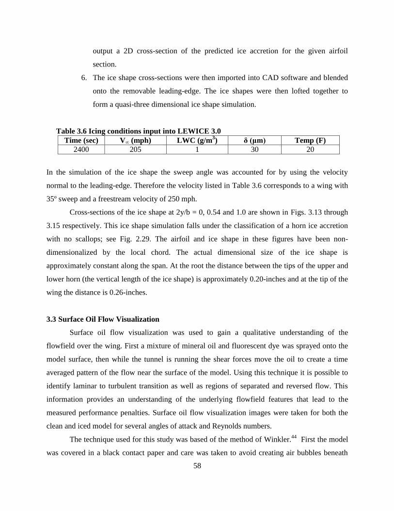
58

output a 2D cross-section of the predicted ice accretion for the given airfoil

section.

6. The ice shape cross-sections were then imported into CAD software and blended

onto the removable leading-edge. The ice shapes were then lofted together to

form a quasi-three dimensional ice shape simulation.

Table 3.6 Icing conditions input into LEWICE 3.0

Time (sec) V∞ (mph) LWC (g/m3) δ (μm) Temp (F)

2400 205 1 30 20

In the simulation of the ice shape the sweep angle was accounted for by using the velocity

normal to the leading-edge. Therefore the velocity listed in Table 3.6 corresponds to a wing with

35º sweep and a freestream velocity of 250 mph.

Cross-sections of the ice shape at 2y/b = 0, 0.54 and 1.0 are shown in Figs. 3.13 through

3.15 respectively. This ice shape simulation falls under the classification of a horn ice accretion

with no scallops; see Fig. 2.29. The airfoil and ice shape in these figures have been non-

dimensionalized by the local chord. The actual dimensional size of the ice shape is

approximately constant along the span. At the root the distance between the tips of the upper and

lower horn (the vertical length of the ice shape) is approximately 0.20-inches and at the tip of the

wing the distance is 0.26-inches.

3.3 Surface Oil Flow Visualization

Surface oil flow visualization was used to gain a qualitative understanding of the

flowfield over the wing. First a mixture of mineral oil and fluorescent dye was sprayed onto the

model surface, then while the tunnel is running the shear forces move the oil to create a time

averaged pattern of the flow near the surface of the model. Using this technique it is possible to

identify laminar to turbulent transition as well as regions of separated and reversed flow. This

information provides an understanding of the underlying flowfield features that lead to the

measured performance penalties. Surface oil flow visualization images were taken for both the

clean and iced model for several angles of attack and Reynolds numbers.

The technique used for this study was based of the method of Winkler.44

First the model

was covered in a black contact paper and care was taken to avoid creating air bubbles beneath

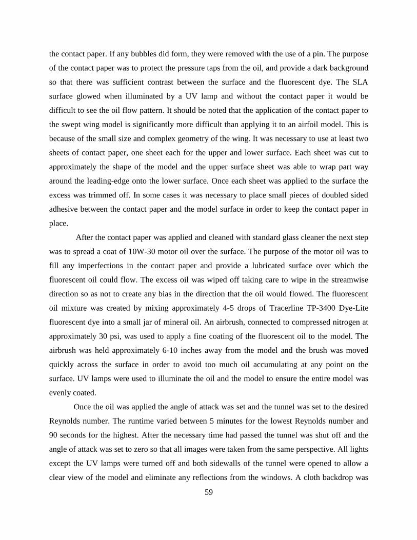
59

the contact paper. If any bubbles did form, they were removed with the use of a pin. The purpose

of the contact paper was to protect the pressure taps from the oil, and provide a dark background

so that there was sufficient contrast between the surface and the fluorescent dye. The SLA

surface glowed when illuminated by a UV lamp and without the contact paper it would be

difficult to see the oil flow pattern. It should be noted that the application of the contact paper to

the swept wing model is significantly more difficult than applying it to an airfoil model. This is

because of the small size and complex geometry of the wing. It was necessary to use at least two

sheets of contact paper, one sheet each for the upper and lower surface. Each sheet was cut to

approximately the shape of the model and the upper surface sheet was able to wrap part way

around the leading-edge onto the lower surface. Once each sheet was applied to the surface the

excess was trimmed off. In some cases it was necessary to place small pieces of doubled sided

adhesive between the contact paper and the model surface in order to keep the contact paper in

place.

After the contact paper was applied and cleaned with standard glass cleaner the next step

was to spread a coat of 10W-30 motor oil over the surface. The purpose of the motor oil was to

fill any imperfections in the contact paper and provide a lubricated surface over which the

fluorescent oil could flow. The excess oil was wiped off taking care to wipe in the streamwise

direction so as not to create any bias in the direction that the oil would flowed. The fluorescent

oil mixture was created by mixing approximately 4-5 drops of Tracerline TP-3400 Dye-Lite

fluorescent dye into a small jar of mineral oil. An airbrush, connected to compressed nitrogen at

approximately 30 psi, was used to apply a fine coating of the fluorescent oil to the model. The

airbrush was held approximately 6-10 inches away from the model and the brush was moved

quickly across the surface in order to avoid too much oil accumulating at any point on the

surface. UV lamps were used to illuminate the oil and the model to ensure the entire model was

evenly coated.

Once the oil was applied the angle of attack was set and the tunnel was set to the desired

Reynolds number. The runtime varied between 5 minutes for the lowest Reynolds number and

90 seconds for the highest. After the necessary time had passed the tunnel was shut off and the

angle of attack was set to zero so that all images were taken from the same perspective. All lights

except the UV lamps were turned off and both sidewalls of the tunnel were opened to allow a

clear view of the model and eliminate any reflections from the windows. A cloth backdrop was

60

then placed behind the model to eliminate any extraneous light from various sources in the lab.

The flow pattern on the model was then imaged using a Nikon Model D3100 digital camera. The

aperture and exposure time were adjusted as necessary to generate the best image. Finally, the oil

was removed from the model with paper towels and glass cleaner and the process was repeated

for the next case.

61

3.4 Figures

Fig. 3.2 Common Research Model.31

Fig. 3.1 Illustration of wind tunnel facility.

62

Fig. 3.3 Steel frame for wind tunnel model.

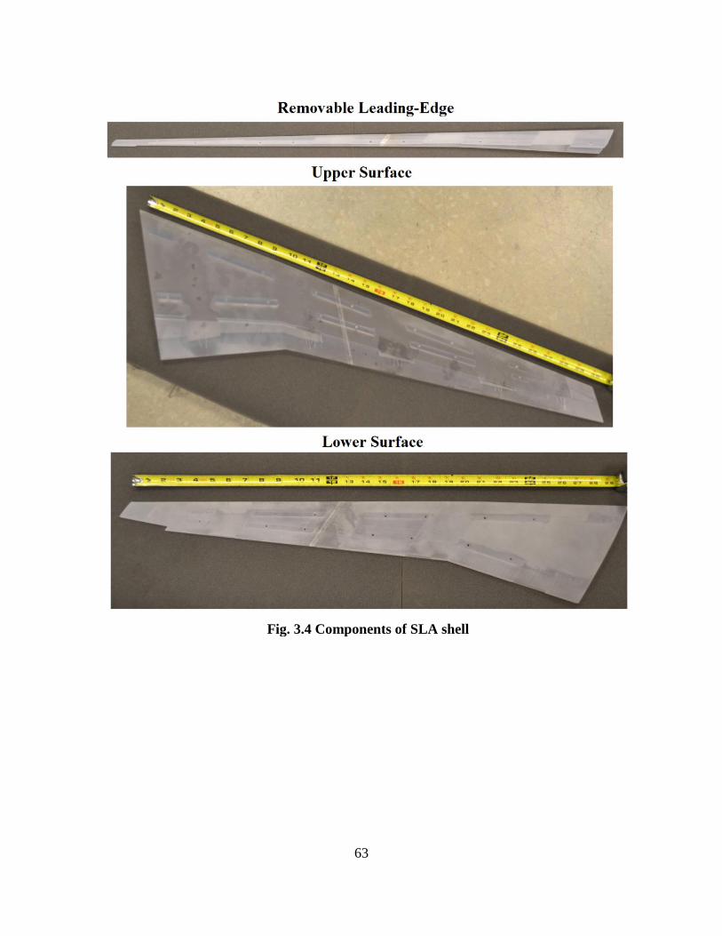
63

Fig. 3.4 Components of SLA shell

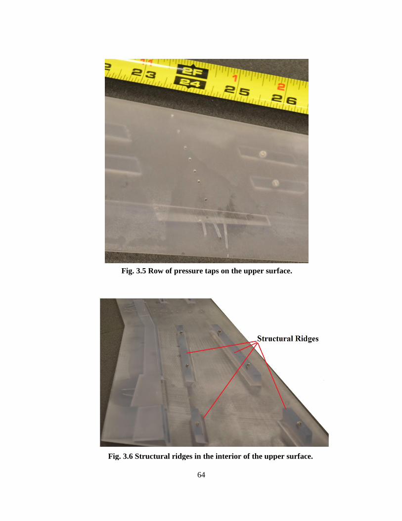
64

Fig. 3.6 Structural ridges in the interior of the upper surface.

Fig. 3.5 Row of pressure taps on the upper surface.

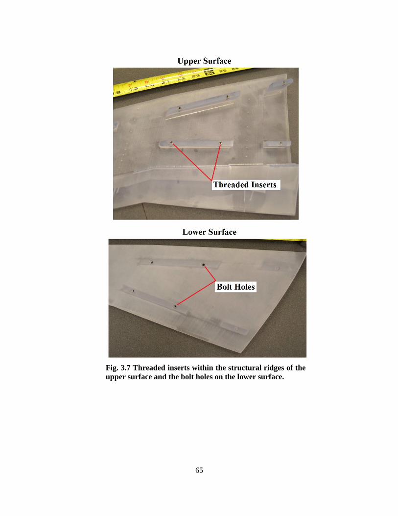
65

Fig. 3.7 Threaded inserts within the structural ridges of the

upper surface and the bolt holes on the lower surface.

66

Fig. 3.8 Important features of the steel frame. Note that one

leading-edge tab is not shown.

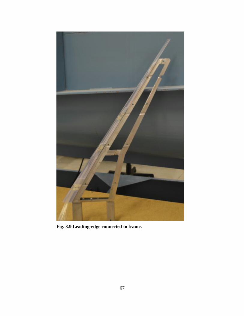
67

Fig. 3.9 Leading-edge connected to frame.

68

Fig. 3.10 Photograph of model connected to the force balance.

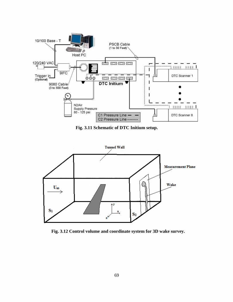
69

Fig. 3.11 Schematic of DTC Initium setup.

Fig. 3.12 Control volume and coordinate system for 3D wake survey.

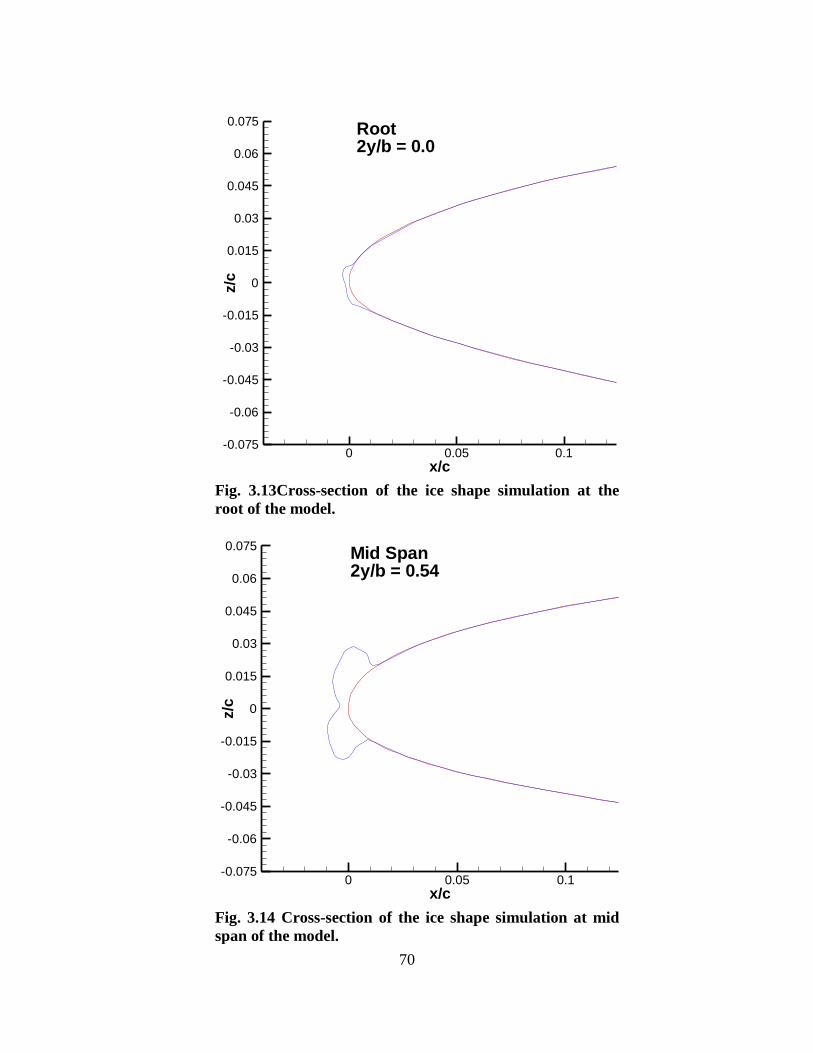
70

x/c

z/c

0 0.05 0.1-0.075

-0.06

-0.045

-0.03

-0.015

0

0.015

0.03

0.045

0.06

0.075Root2y/b = 0.0

Fig. 3.13Cross-section of the ice shape simulation at the

root of the model.

x/c

z/c

0 0.05 0.1-0.075

-0.06

-0.045

-0.03

-0.015

0

0.015

0.03

0.045

0.06

0.075Mid Span2y/b = 0.54

Fig. 3.14 Cross-section of the ice shape simulation at mid

span of the model.

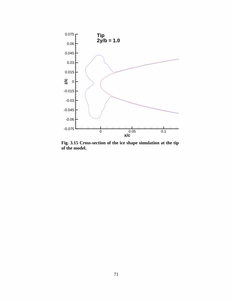
71

x/c

z/c

0 0.05 0.1-0.075

-0.06

-0.045

-0.03

-0.015

0

0.015

0.03

0.045

0.06

0.075 Tip2y/b = 1.0

Fig. 3.15 Cross-section of the ice shape simulation at the tip

of the model.

72

Chapter 4

Results and Discussion

In this chapter the various experimental methods described in the previous chapter will be

used to investigate the effects of the ice on the aerodynamics of the swept wing model. The goal

is to answer several questions. How does the ice influence the performance of the wing? How is

the stalling process influenced? What are the underlying flow features that cause the observed

performance penalty? What effect does the Reynolds number have on the aerodynamics of the

iced wing? These questions will be answered by first presenting an overview of the general

features of the flowfield for the clean and iced wing. This will be followed by a discussion of the

force balance results and then a detailed comparison of the aerodynamics of the clean and iced

wing for selected angles of attack. Finally, the Reynolds number effects will be discussed.

4.1 General Flowfield Overview

This section will present and discuss flow visualization results for the clean and iced

wing over a range of angles of attack. The purpose of this section is to provide a general

overview of the flowfield for both wings and to discuss several of the important features. This

will provide a basis for understanding the performance and more detailed comparisons of the

clean and iced wing discussed in subsequent sections. A similar but brief discussion of the

flowfield for the clean and iced wing that contains pressure sensitive paints results is given by

Diebold et. al.45

All oil flow images in this first section were acquired at a Reynolds number of

3x105 but the basic flowfield features with the exception of a few cases are not significantly

affected by the Reynolds number particularly below stall. It should be noted that for all oil flow

results presented here the first 10% of the span has been removed from the image. For reference,

the Yehudi break is located at 30% of the total span.

4.1.1 Clean Wing Flowfield

Oil flow images for the clean wing at several angles of attack, below stall, for a Reynolds

number of 3x105 are shown in Fig. 4.1. This figure shows that the flowfield of the clean wing

changes significantly with angle of attack at this Reynolds number. At α = 2.3º, along most of

the span a region of low shear or separated flow had developed near approximately 50% chord.

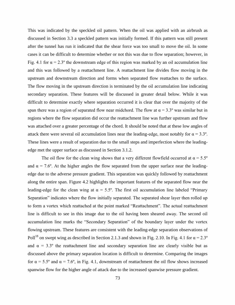
73

This was indicated by the speckled oil pattern. When the oil was applied with an airbrush as

discussed in Section 3.3 a speckled pattern was initially formed. If this pattern was still present

after the tunnel has run it indicated that the shear force was too small to move the oil. In some

cases it can be difficult to determine whether or not this was due to flow separation; however, in

Fig. 4.1 for α = 2.3º the downstream edge of this region was marked by an oil accumulation line

and this was followed by a reattachment line. A reattachment line divides flow moving in the

upstream and downstream direction and forms when separated flow reattaches to the surface.

The flow moving in the upstream direction is terminated by the oil accumulation line indicating

secondary separation. These features will be discussed in greater detail below. While it was

difficult to determine exactly where separation occurred it is clear that over the majority of the

span there was a region of separated flow near midchord. The flow at α = 3.3º was similar but in

regions where the flow separation did occur the reattachment line was further upstream and flow

was attached over a greater percentage of the chord. It should be noted that at these low angles of

attack there were several oil accumulation lines near the leading-edge, most notably for α = 3.3º.

These lines were a result of separation due to the small steps and imperfection where the leading-

edge met the upper surface as discussed in Section 3.1.2.

The oil flow for the clean wing shows that a very different flowfield occurred at α = 5.5º

and α = 7.6º. At the higher angles the flow separated from the upper surface near the leading-

edge due to the adverse pressure gradient. This separation was quickly followed by reattachment

along the entire span. Figure 4.2 highlights the important features of the separated flow near the

leading-edge for the clean wing at α = 5.5º. The first oil accumulation line labeled “Primary

Separation” indicates where the flow initially separated. The separated shear layer then rolled up

to form a vortex which reattached at the point marked “Reattachment”. The actual reattachment

line is difficult to see in this image due to the oil having been sheared away. The second oil

accumulation line marks the “Secondary Separation” of the boundary layer under the vortex

flowing upstream. These features are consistent with the leading-edge separation observations of

Poll18

on swept wing as described in Section 2.1.3 and shown in Fig. 2.10. In Fig. 4.1 for α = 2.3º

and α = 3.3º the reattachment line and secondary separation line are clearly visible but as

discussed above the primary separation location is difficult to determine. Comparing the images

for α = 5.5º and α = 7.6º, in Fig. 4.1, downstream of reattachment the oil flow shows increased

spanwise flow for the higher angle of attack due to the increased spanwise pressure gradient.

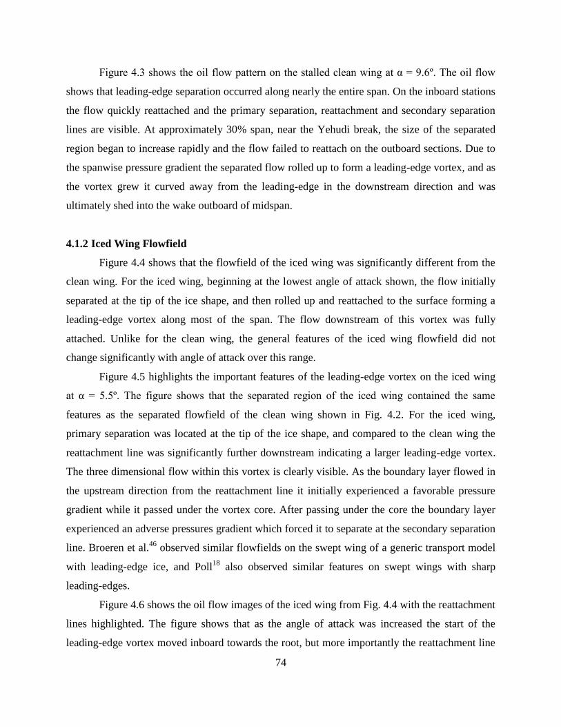
74

Figure 4.3 shows the oil flow pattern on the stalled clean wing at α = 9.6º. The oil flow

shows that leading-edge separation occurred along nearly the entire span. On the inboard stations

the flow quickly reattached and the primary separation, reattachment and secondary separation

lines are visible. At approximately 30% span, near the Yehudi break, the size of the separated

region began to increase rapidly and the flow failed to reattach on the outboard sections. Due to

the spanwise pressure gradient the separated flow rolled up to form a leading-edge vortex, and as

the vortex grew it curved away from the leading-edge in the downstream direction and was

ultimately shed into the wake outboard of midspan.

4.1.2 Iced Wing Flowfield

Figure 4.4 shows that the flowfield of the iced wing was significantly different from the

clean wing. For the iced wing, beginning at the lowest angle of attack shown, the flow initially

separated at the tip of the ice shape, and then rolled up and reattached to the surface forming a

leading-edge vortex along most of the span. The flow downstream of this vortex was fully

attached. Unlike for the clean wing, the general features of the iced wing flowfield did not

change significantly with angle of attack over this range.

Figure 4.5 highlights the important features of the leading-edge vortex on the iced wing

at α = 5.5º. The figure shows that the separated region of the iced wing contained the same

features as the separated flowfield of the clean wing shown in Fig. 4.2. For the iced wing,

primary separation was located at the tip of the ice shape, and compared to the clean wing the

reattachment line was significantly further downstream indicating a larger leading-edge vortex.

The three dimensional flow within this vortex is clearly visible. As the boundary layer flowed in

the upstream direction from the reattachment line it initially experienced a favorable pressure

gradient while it passed under the vortex core. After passing under the core the boundary layer

experienced an adverse pressures gradient which forced it to separate at the secondary separation

line. Broeren et al.46

observed similar flowfields on the swept wing of a generic transport model

with leading-edge ice, and Poll18

also observed similar features on swept wings with sharp

leading-edges.

Figure 4.6 shows the oil flow images of the iced wing from Fig. 4.4 with the reattachment

lines highlighted. The figure shows that as the angle of attack was increased the start of the

leading-edge vortex moved inboard towards the root, but more importantly the reattachment line

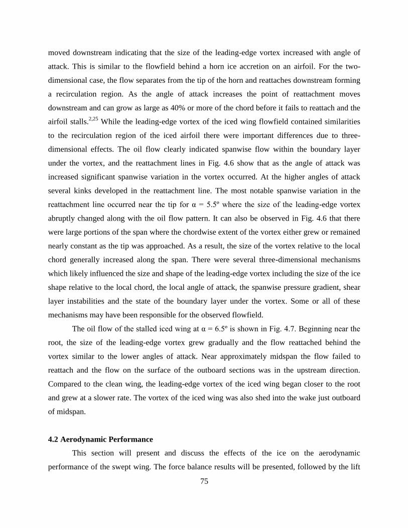
75

moved downstream indicating that the size of the leading-edge vortex increased with angle of

attack. This is similar to the flowfield behind a horn ice accretion on an airfoil. For the two-

dimensional case, the flow separates from the tip of the horn and reattaches downstream forming

a recirculation region. As the angle of attack increases the point of reattachment moves

downstream and can grow as large as 40% or more of the chord before it fails to reattach and the

airfoil stalls.2,25

While the leading-edge vortex of the iced wing flowfield contained similarities

to the recirculation region of the iced airfoil there were important differences due to three-

dimensional effects. The oil flow clearly indicated spanwise flow within the boundary layer

under the vortex, and the reattachment lines in Fig. 4.6 show that as the angle of attack was

increased significant spanwise variation in the vortex occurred. At the higher angles of attack

several kinks developed in the reattachment line. The most notable spanwise variation in the

reattachment line occurred near the tip for α = 5.5º where the size of the leading-edge vortex

abruptly changed along with the oil flow pattern. It can also be observed in Fig. 4.6 that there

were large portions of the span where the chordwise extent of the vortex either grew or remained

nearly constant as the tip was approached. As a result, the size of the vortex relative to the local

chord generally increased along the span. There were several three-dimensional mechanisms

which likely influenced the size and shape of the leading-edge vortex including the size of the ice

shape relative to the local chord, the local angle of attack, the spanwise pressure gradient, shear

layer instabilities and the state of the boundary layer under the vortex. Some or all of these

mechanisms may have been responsible for the observed flowfield.

The oil flow of the stalled iced wing at α = 6.5º is shown in Fig. 4.7. Beginning near the

root, the size of the leading-edge vortex grew gradually and the flow reattached behind the

vortex similar to the lower angles of attack. Near approximately midspan the flow failed to

reattach and the flow on the surface of the outboard sections was in the upstream direction.

Compared to the clean wing, the leading-edge vortex of the iced wing began closer to the root

and grew at a slower rate. The vortex of the iced wing was also shed into the wake just outboard

of midspan.

4.2 Aerodynamic Performance

This section will present and discuss the effects of the ice on the aerodynamic

performance of the swept wing. The force balance results will be presented, followed by the lift

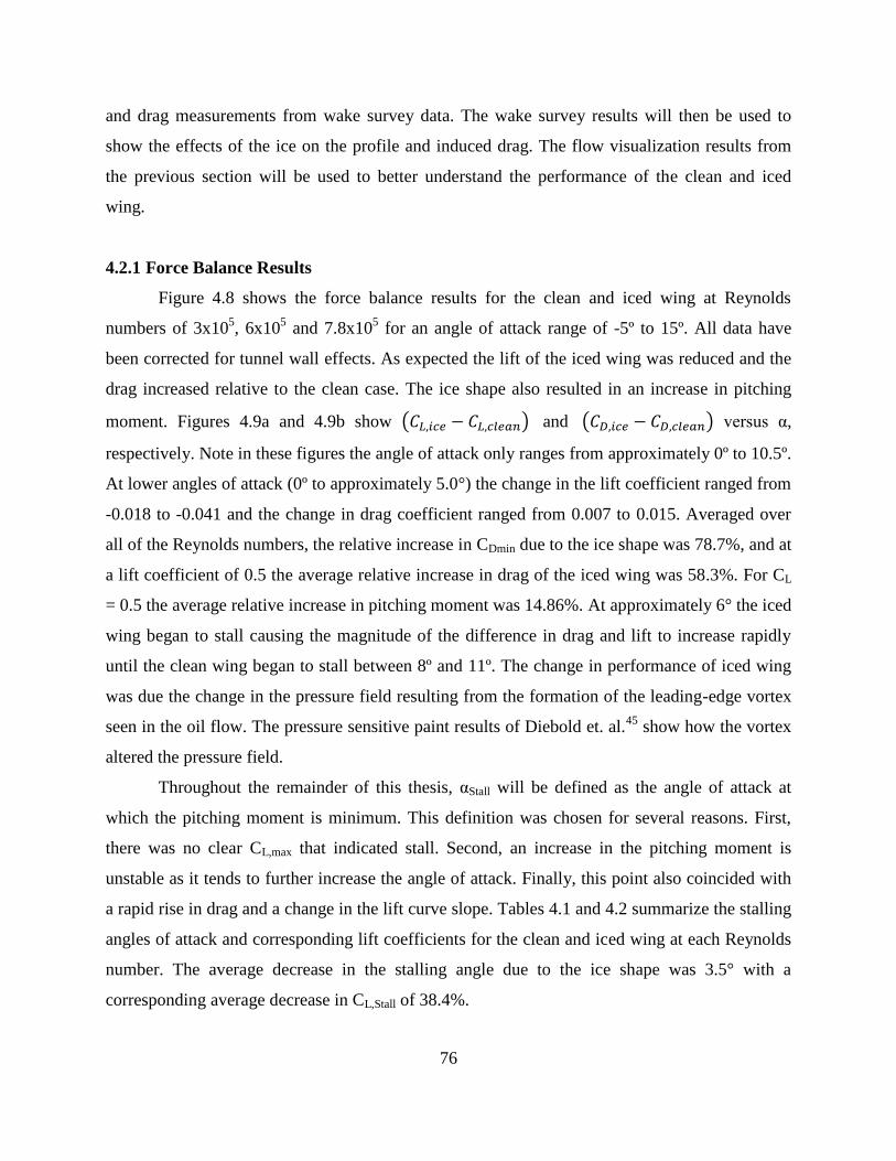
76

and drag measurements from wake survey data. The wake survey results will then be used to

show the effects of the ice on the profile and induced drag. The flow visualization results from

the previous section will be used to better understand the performance of the clean and iced

wing.

4.2.1 Force Balance Results

Figure 4.8 shows the force balance results for the clean and iced wing at Reynolds

numbers of 3x105, 6x10

5 and 7.8x10

5 for an angle of attack range of -5º to 15º. All data have

been corrected for tunnel wall effects. As expected the lift of the iced wing was reduced and the

drag increased relative to the clean case. The ice shape also resulted in an increase in pitching

moment. Figures 4.9a and 4.9b show ( ) and ( ) versus α,

respectively. Note in these figures the angle of attack only ranges from approximately 0º to 10.5º.

At lower angles of attack (0º to approximately 5.0°) the change in the lift coefficient ranged from

-0.018 to -0.041 and the change in drag coefficient ranged from 0.007 to 0.015. Averaged over

all of the Reynolds numbers, the relative increase in CDmin due to the ice shape was 78.7%, and at

a lift coefficient of 0.5 the average relative increase in drag of the iced wing was 58.3%. For CL

= 0.5 the average relative increase in pitching moment was 14.86%. At approximately 6° the iced

wing began to stall causing the magnitude of the difference in drag and lift to increase rapidly

until the clean wing began to stall between 8º and 11º. The change in performance of iced wing

was due the change in the pressure field resulting from the formation of the leading-edge vortex

seen in the oil flow. The pressure sensitive paint results of Diebold et. al.45

show how the vortex

altered the pressure field.

Throughout the remainder of this thesis, αStall will be defined as the angle of attack at

which the pitching moment is minimum. This definition was chosen for several reasons. First,

there was no clear CL,max that indicated stall. Second, an increase in the pitching moment is

unstable as it tends to further increase the angle of attack. Finally, this point also coincided with

a rapid rise in drag and a change in the lift curve slope. Tables 4.1 and 4.2 summarize the stalling

angles of attack and corresponding lift coefficients for the clean and iced wing at each Reynolds

number. The average decrease in the stalling angle due to the ice shape was 3.5° with a

corresponding average decrease in CL,Stall of 38.4%.

77

Table 4.1 αStall and CL,Stall for the clean wing. (Stall defined at CM,min)

Re (x105) αStall CL,Stall

3.0 8.60 0.70

6.0 9.65 0.78

7.8 10.2 0.82

Table 4.2 αStall and CL,Stall for the ice wing. (Stall defined at CM,min)

Re (x105) αStall CL,Stall

3.0 5.95 0.53

6.0 5.98 0.56

7.8 5.98 0.57

From the balance data it can be seen that both the clean and iced wing underwent a gentle

stalling process, as there was no sudden decrease in lift. A gentle stall resulted from the fact that

only a portion of the wing stalled as shown in the oil flow. The inboard sections of the wing were

still producing a significant amount of lift as will be seen using the wake survey results. The

increase in pitching moment indicates that the stalling process began on the outboard sections of

the wing. This was consistent with the oil flow visualization images shown in Fig. 4.3 for the

clean wing and Fig. 4.7 for the iced wing. When the outboard sections stalled the center of

pressure shifted forward resulting in an increase in the pitching moment.

4.2.2 Wake Survey Integrated Performance Results

This section will present and discuss the wake survey results for the total lift and drag as

well as the profile and induced drag. The wake survey results were corrected using the same

correction factors as for the balance data. For the clean wing, wake surveys were performed from

α = 2.3º to 10.6º and for the iced wing from α = 2.3º to 6.5º. Figures 4.10a and 4.11a compare the

total lift measured by the force balance and wake survey techniques for the clean and iced wing,

respectively, at a Reynolds number of 6x105. Figures 4.10b and 4.11b show the corresponding

comparisons for drag. For both the clean and iced wing, the results showed that the total lift and

the lift curve slope calculated by the wake survey were consistently higher than the balance lift.

This was unexpected considering that the inboard 15% of the span was not surveyed. The reason

for this error is unknown although it is likely due to error in the vorticity calculations.

Throughout the range of angles tested, the mean errors in the lift coefficient for the clean and

78

iced wing were 5.1% and 5.6%, respectively. The wake survey did appear to accurately capture

the effect of stall on the lift.

The drag measured by the wake survey, Figs. 4.10b and 4.11b, was consistently less than

the balance drag; however, the drag curve from the wake measurements closely follows that of

the balance measurements. The change in drag due to stall was accurately captured by the wake

survey. The drag results from the wake survey were consistent with the entire wake not being

surveyed. The mean error in the drag measured by the wake survey was 11.2% and 4.3% for the

clean and iced wing respectively. The higher error for the clean wing was likely due to error in

the induced drag resulting from uncertainty in the vorticity calculation. As will be seen below,

the induced drag of the clean wing was a larger percentage of the total drag than for the iced

wing. This may have resulted in a larger total error in the clean wing drag coefficient. The results

presented in Figs. 4.10 and 4.11 demonstrate that the wake survey provides reasonable

measurements of the lift and drag although there is still room for improvement.

The profile and induced drag coefficients versus angle of attack for the clean and iced

wing are shown in Fig. 4.12. The results show that the profile drag of the iced wing was

significantly higher than that of the clean wing. This is consistent with the oil flow visualization

discussed in Section 4.1.2 which showed a large region of separated flow behind the ice shape.

The leading-edge vortex resulting from the flow separation significantly increased the pressure

drag on the wing. Note that the oil flow images discussed above were taken at Re = 3x105 and

the wake survey data discussed here were taken at Re = 6x105. While there were some changes

in performance due to change in Reynolds number, the large scale features of the flow field were

relatively unchanged. Oil flow images at a higher Reynolds number will be discussed below. In

Fig. 4.12 it can be seen that the rate of increase of the profile drag with angle of attack for the

iced wing was higher than for the clean wing. This was due to the increasing size of the

separated region as shown in Fig. 4.6. Figure 4.12 shows that the induced drag of the wing was

only slightly reduced by the presence of the ice shape. This was likely due to the small reduction

in lift caused by the ice at a given angle of attack. This indicates that the ice shape did not

significantly affect the total amount of streamwise vorticity shed into the wake. At the lowest

angle of attack, α = 2.3º, the induced drag made up 29.1% and 16.4% of the total drag for the

clean and iced wing, respectively. As the angle of attack increased, the induced drag of the iced

wing became a maximum of 25.1% of the total drag at α = 4.4º, and for the clean wing the

79

induced drag increased to 49.5% of the total drag at α = 7.6º. As the clean and iced wing began

to stall, the profile drag increased rapidly but the total induced drag appeared unaffected by stall.

Overall the ice had a significant effect on the performance of the wing. The drag was

increased throughout the entire range of angles of attack and the stalling angle and lift coefficient

were reduced. By using the flow visualization along with the force balance results a better

understanding of why the performance degraded was obtained. The wake survey results were

used to gain a more complete understanding of how the drag was influenced by the ice.

4.3 Detailed Comparisons

Despite the discussion above there is still a great deal to learn about the aerodynamics of

this swept wing with ice. It was seen that the surface flowfield was extremely three dimensional.

It is expected that the pressure field, load distributions and wakes are also three dimensional. In

order to gain a better understanding of the swept wing with ice it is necessary to investigate the

three dimensional aspects of the flow. This section will use flow visualization, Cp distributions

and wake survey results in order to provide detailed comparisons of the aerodynamics of the

clean and iced wings at selected angles of attack. The purpose of this section is to utilize all of

the experimental methods discussed above in order to learn how the ice influences the local

aerodynamics along the span, and how these changes affect the total performance. Features seen

in the oil flow will be compared to features seen in the wake, and the effect of these features on

the load distribution will be discussed. The data presented in this section was acquired at a

Reynolds number of 6x105.

4.3.1 Comparison of Clean and Iced Wing at α = 3.3º

Figure 4.13 compares the oil flow for the clean and iced wing at α = 3.3º and Re = 6x105.

The images show that the flowfield of the clean wing was significantly more affected by the

imperfections in the surface than the iced wing. Many of the oil accumulation lines near the

leading-edge of the clean wing were a result of the steps in the surface. Downstream of the

leading-edge region however the flow on the clean wing was mostly attached except near the tip.

In the tip region of the clean wing a separated region formed near midchord similar to the lower

Reynolds number case. The separated region was only a few percent of the local chord and the

flow quickly reattached. For the iced wing, the flow separated from the tip of the ice shape

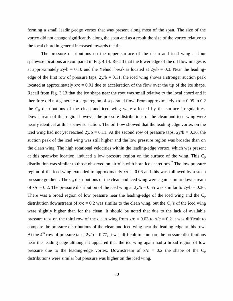
80

forming a small leading-edge vortex that was present along most of the span. The size of the

vortex did not change significantly along the span and as a result the size of the vortex relative to

the local chord in general increased towards the tip.

The pressure distributions on the upper surface of the clean and iced wing at four

spanwise locations are compared in Fig. 4.14. Recall that the lower edge of the oil flow images is

at approximately 2y/b = 0.10 and the Yehudi break is located at 2y/b = 0.3. Near the leading-

edge of the first row of pressure taps, 2y/b = 0.11, the iced wing shows a stronger suction peak

located at approximately x/c = 0.01 due to acceleration of the flow over the tip of the ice shape.

Recall from Fig. 3.13 that the ice shape near the root was small relative to the local chord and it

therefore did not generate a large region of separated flow. From approximately x/c = 0.05 to 0.2

the Cp distributions of the clean and iced wing were affected by the surface irregularities.

Downstream of this region however the pressure distributions of the clean and iced wing were

nearly identical at this spanwise station. The oil flow showed that the leading-edge vortex on the

iced wing had not yet reached 2y/b = 0.11. At the second row of pressure taps, 2y/b = 0.36, the

suction peak of the iced wing was still higher and the low pressure region was broader than on

the clean wing. The high rotational velocities within the leading-edge vortex, which was present

at this spanwise location, induced a low pressure region on the surface of the wing. This Cp

distribution was similar to those observed on airfoils with horn ice accretions.2 The low pressure

region of the iced wing extended to approximately x/c = 0.06 and this was followed by a steep

pressure gradient. The Cp distributions of the clean and iced wing were again similar downstream

of x/c = 0.2. The pressure distribution of the iced wing at 2y/b = 0.55 was similar to 2y/b = 0.36.

There was a broad region of low pressure near the leading-edge of the iced wing and the Cp

distribution downstream of x/c = 0.2 was similar to the clean wing, but the Cp’s of the iced wing

were slightly higher than for the clean. It should be noted that due to the lack of available

pressure taps on the third row of the clean wing from x/c = 0.03 to x/c = 0.2 it was difficult to

compare the pressure distributions of the clean and iced wing near the leading-edge at this row.

At the 4th

row of pressure taps, 2y/b = 0.77, it was difficult to compare the pressure distributions

near the leading-edge although it appeared that the ice wing again had a broad region of low

pressure due to the leading-edge vortex. Downstream of x/c = 0.2 the shape of the Cp

distributions were similar but pressure was higher on the iced wing.

81

Figures 4.15a and 4.15b show the wake of the clean and iced wing respectively. Contours

represent axial velocity normalized by the freestream while the vectors represent the transverse

velocity. The transverse velocity refers to the total velocity component perpendicular to the

freestream. It can be seen that the wake of the iced wing was significantly thicker than that of the

clean wing which was consistent with the higher drag measured by the balance. In addition, the

axial velocity contours show that the thickness of the iced wing wake increased along the span.

Near the root, the thicknesses of the two wakes were similar, but as the tip was approached the

size of the iced wing wake increased. The oil flow showed that the size of the separated region

behind the ice shape increased relative to the local chord as the tip was approached, and the five-

hole probe measurements show that this resulted in a thicker wake. Comparing the clean and iced

tip vortex several differences were observed. First, the maximum transverse velocity within the

clean wing tip vortex was approximately 0.14U∞ while for the iced wing the maximum was

0.1U∞. Reduced tip vortex strength was consistent with the smaller lift produced by the iced

wing. Secondly, the boundary of the clean wing tip vortex was more clearly defined than for the

iced wing. For the clean wing, the rollup of the wake was clearly visible; however, for the iced

wing there was merging between the tip vortex and the rest of the wake and the rollup process

was not as clear. This may have been due to increased turbulent mixing caused by entrainment of

separated flow into the vortex. Finally, there was a large region of low axial velocity within the

tip vortex of the iced wing, which may have been due to the entrainment of low momentum

separated flow into the vortex.

In order to better understand the flowfield it was useful to relate features seen in the

farfield to the flow over the wing. Figure 4.16 shows the oil flow and wake of the iced wing at α

= 3.3º. Note that the scale of the axial velocity contours in the wake have been adjusted in order

to accentuate certain features. The reattachment line of the leading-edge vortex has been

highlighted, and there are arrows indicating where on the surface of the wing certain features in

the wake may have originated. It should be noted that the exact point of origin is difficult to

determine due to wake rollup. The oil flow image shows several small kinks in the reattachment

line of the leading-edge vortex, and the two images together suggest that the phenomena

responsible for these kinks lead to localized regions of comparatively larger momentum deficit in

the wake. As discussed in Section 4.1.2 there were numerous three-dimensional mechanisms that

could influence the size of the leading-edge vortex including shear layer instabilities and the state

82

of the boundary layer under the vortex; however, to determine the cause it would be necessary to

perform off surface measurements such as PIV.

The spanwise distributions of Cl, Cd, Cdp and Cdi for the clean and iced at α = 3.3º are

compared in Figs. 4.17a-d respectively. Cdp and Cdi represent the sectional profile and induced

drag respectively. Note that only every other point of the distribution is shown. At α = 3.3º and

Re = 6x105

the lift and drag coefficient of the clean wing were 0.421 and 0.0230, respectively,

and for the iced wing 0.396 and 0.0317, respectively. The lift distribution of the clean and iced

wing both show that the outboard sections of the wing were more heavily loaded than the

inboard sections consistent with the aerodynamics of a swept wing as discussed in Section 2.1.1.

The higher sectional lift coefficients implied a higher induced angle of attack on the outboard

sections. The higher angle of attack and larger relative size of the ice shape help explain why the

vortex was generally larger on the outboard sections. The shapes of the clean and iced lift

distributions were similar; however, as the tip was approached the sectional lift coefficient of the

iced wing decreased relative to that of the clean wing. Figure 4.16b shows that the sectional drag

coefficient of the iced wing was greater than that of the clean wing across the entire portion of

the span that was surveyed. In addition, as the tip was approached the sectional drag coefficient

of the iced wing increased faster than for the clean wing. Figures 4.16c and 4.16d show that this

increase in the total sectional drag coefficient was the result of a rapid increase in the profile drag

coefficient along the span while the sectional induced drag of the two wings was nearly equal

along most of the span. These results were consistent with the oil flow visualization shown in

Fig. 4.13. As the size of the leading-edge vortex grew relative to the local chord, the impact on

the local aerodynamics increased. A larger separated region reduced the local circulation and

increased the pressure drag resulting in decreased sectional lift coefficients and increased profile

drag. The increased profile drag of the iced wing was responsible for the thicker wake seen in

Fig. 4.15b.

In Fig. 4.17b, several peaks in the sectional drag coefficient distribution can be seen. The

most prominent peak, located near 2y/b = 1.0, was due to the tip vortex and will be discussed

shortly. It is interesting to note that the four peaks in the iced wing drag distribution located near

2y/b = 0.30, 0.59, 0.74 and 0.90 correspond to the kinks in the reattachment lines and features

observed in the wake highlighted in Fig. 4.16. Figures 4.17c and 4.17d show that these peaks

were primarily due to contributions from profile drag although there were small peaks in the

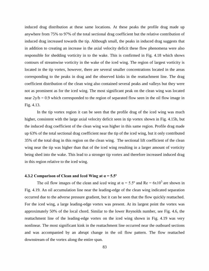
83

induced drag distribution at these same locations. At these peaks the profile drag made up

anywhere from 75% to 97% of the total sectional drag coefficient but the relative contribution of

induced drag increased towards the tip. Although small, the peaks in induced drag suggests that

in addition to creating an increase in the axial velocity deficit these flow phenomena were also

responsible for shedding vorticity in to the wake. This is confirmed in Fig. 4.18 which shows

contours of streamwise vorticity in the wake of the iced wing. The region of largest vorticity is

located in the tip vortex, however, there are several smaller concentrations located in the areas

corresponding to the peaks in drag and the observed kinks in the reattachment line. The drag

coefficient distribution of the clean wing also contained several peaks and valleys but they were

not as prominent as for the iced wing. The most significant peak on the clean wing was located

near 2y/b = 0.9 which corresponded to the region of separated flow seen in the oil flow image in

Fig. 4.13.

In the tip vortex region it can be seen that the profile drag of the iced wing was much

higher, consistent with the large axial velocity deficit seen in tip vortex shown in Fig. 4.15b, but

the induced drag coefficient of the clean wing was higher in this same region. Profile drag made

up 63% of the total sectional drag coefficient near the tip of the iced wing, but it only contributed

35% of the total drag in this region on the clean wing. The sectional lift coefficient of the clean

wing near the tip was higher than that of the iced wing resulting in a larger amount of vorticity

being shed into the wake. This lead to a stronger tip vortex and therefore increased induced drag

in this region relative to the iced wing.

4.3.2 Comparison of Clean and Iced Wing at α = 5.5º

The oil flow images of the clean and iced wing at α = 5.5º and Re = 6x105

are shown in

Fig. 4.19. An oil accumulation line near the leading-edge of the clean wing indicated separation

occurred due to the adverse pressure gradient, but it can be seen that the flow quickly reattached.

For the iced wing, a large leading-edge vortex was present. At its largest point the vortex was

approximately 50% of the local chord. Similar to the lower Reynolds number, see Fig. 4.6, the

reattachment line of the leading-edge vortex on the iced wing shown in Fig. 4.19 was very

nonlinear. The most significant kink in the reattachment line occurred near the outboard sections

and was accompanied by an abrupt change in the oil flow pattern. The flow reattached

downstream of the vortex along the entire span.

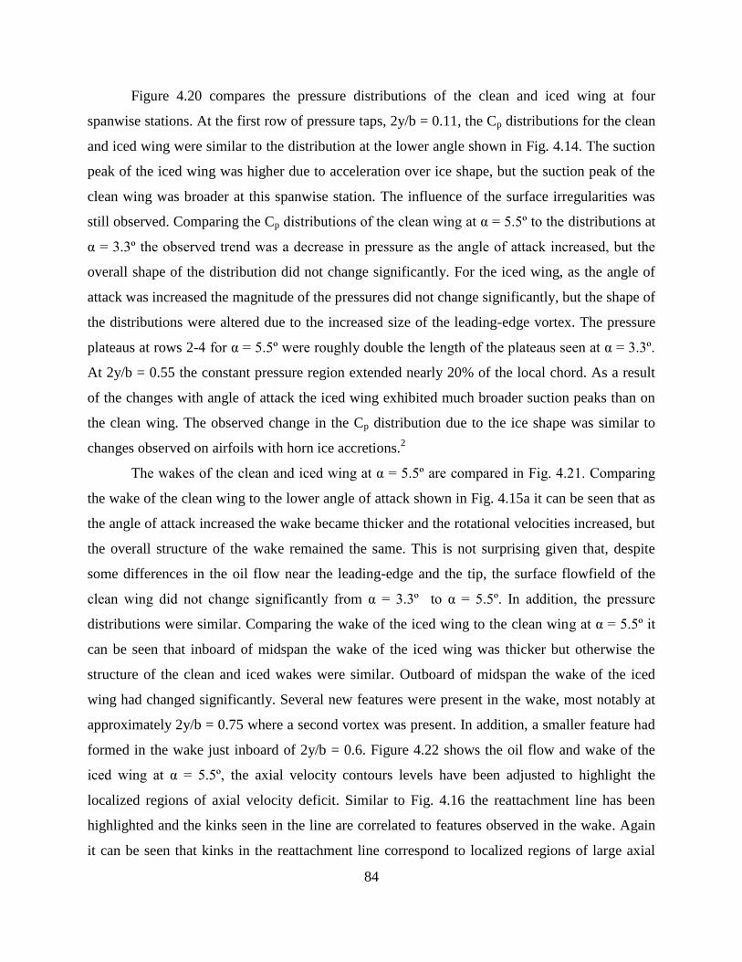
84

Figure 4.20 compares the pressure distributions of the clean and iced wing at four

spanwise stations. At the first row of pressure taps, 2y/b = 0.11, the Cp distributions for the clean

and iced wing were similar to the distribution at the lower angle shown in Fig. 4.14. The suction

peak of the iced wing was higher due to acceleration over ice shape, but the suction peak of the

clean wing was broader at this spanwise station. The influence of the surface irregularities was

still observed. Comparing the Cp distributions of the clean wing at α = 5.5º to the distributions at

α = 3.3º the observed trend was a decrease in pressure as the angle of attack increased, but the

overall shape of the distribution did not change significantly. For the iced wing, as the angle of

attack was increased the magnitude of the pressures did not change significantly, but the shape of

the distributions were altered due to the increased size of the leading-edge vortex. The pressure

plateaus at rows 2-4 for α = 5.5º were roughly double the length of the plateaus seen at α = 3.3º.

At 2y/b = 0.55 the constant pressure region extended nearly 20% of the local chord. As a result

of the changes with angle of attack the iced wing exhibited much broader suction peaks than on

the clean wing. The observed change in the Cp distribution due to the ice shape was similar to

changes observed on airfoils with horn ice accretions.2

The wakes of the clean and iced wing at α = 5.5º are compared in Fig. 4.21. Comparing

the wake of the clean wing to the lower angle of attack shown in Fig. 4.15a it can be seen that as

the angle of attack increased the wake became thicker and the rotational velocities increased, but

the overall structure of the wake remained the same. This is not surprising given that, despite

some differences in the oil flow near the leading-edge and the tip, the surface flowfield of the

clean wing did not change significantly from α = 3.3º to α = 5.5º. In addition, the pressure

distributions were similar. Comparing the wake of the iced wing to the clean wing at α = 5.5º it

can be seen that inboard of midspan the wake of the iced wing was thicker but otherwise the

structure of the clean and iced wakes were similar. Outboard of midspan the wake of the iced

wing had changed significantly. Several new features were present in the wake, most notably at

approximately 2y/b = 0.75 where a second vortex was present. In addition, a smaller feature had

formed in the wake just inboard of 2y/b = 0.6. Figure 4.22 shows the oil flow and wake of the

iced wing at α = 5.5º, the axial velocity contours levels have been adjusted to highlight the

localized regions of axial velocity deficit. Similar to Fig. 4.16 the reattachment line has been

highlighted and the kinks seen in the line are correlated to features observed in the wake. Again

it can be seen that kinks in the reattachment line correspond to localized regions of large axial

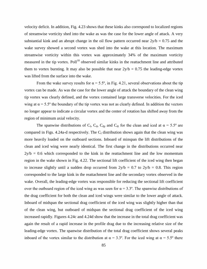
85

velocity deficit. In addition, Fig. 4.23 shows that these kinks also correspond to localized regions

of streamwise vorticity shed into the wake as was the case for the lower angle of attack. A very

substantial kink and an abrupt change in the oil flow pattern occurred near 2y/b = 0.75 and the

wake survey showed a second vortex was shed into the wake at this location. The maximum

streamwise vorticity within this vortex was approximately 34% of the maximum vorticity

measured in the tip vortex. Poll18

observed similar kinks in the reattachment line and attributed

them to vortex bursting. It may also be possible that near 2y/b = 0.75 the leading-edge vortex

was lifted from the surface into the wake.

From the wake survey results for α = 5.5º, in Fig. 4.21, several observations about the tip

vortex can be made. As was the case for the lower angle of attack the boundary of the clean wing

tip vortex was clearly defined, and the vortex contained large transverse velocities. For the iced

wing at α = 5.5º the boundary of the tip vortex was not as clearly defined. In addition the vectors

no longer appear to indicate a circular vortex and the center of rotation has shifted away from the

region of minimum axial velocity.

The spanwise distributions of Cl, Cd, Cdp and Cdi for the clean and iced at α = 5.5º are

compared in Figs. 4.24a-d respectively. The Cl distribution shows again that the clean wing was

more heavily loaded on the outboard sections. Inboard of minspan the lift distributions of the

clean and iced wing were nearly identical. The first change in the distributions occurred near

2y/b = 0.6 which corresponded to the kink in the reattachment line and the low momentum

region in the wake shown in Fig. 4.22. The sectional lift coefficient of the iced wing then began

to increase slightly until a sudden drop occurred from 2y/b = 0.7 to 2y/b = 0.8. This region

corresponded to the large kink in the reattachment line and the secondary vortex observed in the

wake. Overall, the leading-edge vortex was responsible for reducing the sectional lift coefficient

over the outboard region of the iced wing as was seen for α = 3.3º. The spanwise distributions of

the drag coefficient for both the clean and iced wings were similar to the lower angle of attack.

Inboard of midspan the sectional drag coefficient of the iced wing was slightly higher than that

of the clean wing, but outboard of midspan the sectional drag coefficient of the iced wing

increased rapidly. Figures 4.24c and 4.24d show that the increase in the total drag coefficient was

again the result of a rapid increase in the profile drag due to the increasing relative size of the

leading-edge vortex. The spanwise distribution of the total drag coefficient shows several peaks

inboard of the vortex similar to the distribution at α = 3.3º. For the iced wing at α = 5.5º there

86

were peaks in the drag located at 2y/b = 0.57, 0.75 and 0.91. The location of these peaks

corresponded to the kinks in the reattachment line as well as the localized regions of axial

velocity deficit and vorticity shown in Figs. 4.22 and 4.23, respectively. Figure 4.24c shows that

the majority of the contribution to these peaks was from profile drag which made up anywhere

from 73% to 86% of the total sectional drag; however, there were also a small peaks in the

distribution of induced drag for the iced wing at these locations. The largest peak in induced

drag, inboard of the tip vortex, was located at 2y/b = 0.75. This is consistent with the

observations made from Fig. 4.22 that the kink in the reattachment line near 2y/b = 0.75

corresponded to a vortex being shed into the wake. The drag coefficient distribution of the clean

wing did not contain the large peaks seen for the iced wing. Figure 4.24c shows that the profile

drag coefficient of the clean wing was relatively constant across the span until the tip vortex was

reached. The induced drag coefficient increased slowly as the tip was approached due to an

increase in the amount of vorticity being shed into the wake. The drag coefficient distribution of

the clean wing did contain small peaks and valleys but it was difficult to correlate them to

features in the oil flow.

Similar to the lower angle of attack the largest peak in drag occurred near the tip vortex.

At the lower angle of attack, α = 3.3º, the sectional drag coefficient near the tip of the iced wing

was larger than the clean wing due to the high profile drag coefficient; however, at the higher

angle of attack the sectional drag coefficient of the clean wing surpassed the iced wing due to the

strong tip vortex and resulting induced drag. The profile drag contributed 28% and 60% of the

total section drag coefficient within the tip vortex of the clean and iced wing, respectively.

4.3.3 Comparison of Clean and Iced Wing Stalled Flowfield

This section will discuss the flowfield of the clean and iced wing post stall. Since the two

wings stalled at different angles of attack the data are presented for the clean wing at α = 10.7º

and the iced wing at α = 6.5º. As a result, a direct comparison of the relative magnitudes of

quantities such as Cp, Cl and Cd is not as valuable as for previous sections; however, there are

several differences between the flowfields of the stalled clean and iced wing making a qualitative

comparison useful.

The oil flow images for the stalled clean and iced wing at Re = 6x105

are shown in Fig.

4.25. As was shown for the lower Reynolds number in Section 4.1, the stalled flowfields of both

87

wings were dominated by leading-edge vortices. In the case of the clean wing at α = 10.7º a part-

span leading-edge vortex began near midspan and quickly increased in size before ultimately

being shed into the wake in-between 60-70% span. Inboard of the leading-edge vortex the flow

was fully attached but outboard of the vortex the flow over the surface was reversed. This is

similar to part-span leading-edge vortices observed by Poll.18

The stalled flowfield of the iced

wing shown in Fig. 4.25 contained several similarities to the iced wing flowfield at lower angles

of attack. The leading-edge vortex began near the root and increases in size slowly until

approximately midspan. Over the inboard regions the flow reattached behind the vortex as it did

at the lower angles. Near midspan however the flow failed to reattach and the vortex was shed

into the wake. The flow over the surface was reversed from approximately 2y/b = 0.5 to 0.75, but

at 2y/b = 0.75 the abrupt change in the oil flow pattern observed at lower angels of attack was

still present. Over the outboard sections there appeared to be a reattachment line and the flow

was attached over the aft portion of the chord. These flowfield features were consistent with the

balance data which indicated tip stall.

The Cp distributions of the clean and iced wing for several spanwise stations are shown in

Fig. 4.26. At 2y/b = 0.11 and 0.36 the suction over the leading-edge of the clean wing had

increased substantially from the lower angle of attack and the flow was still attached over the

inboard sections. At the third spanwise station the presence of the leading-edge vortex was seen

in the Cp distribution of the clean wing. Compared to the second row, the suction peak had

become broader and the magnitude of the Cp’s were reduced significantly. For the iced wing, the

suction peak over the first row of taps is broader when compared to the lower angles of attack

and the magnitude of the pressure was slightly reduced. At the second row of taps the pressure

plateau of the leading-edge vortex extends nearly 20% of the chord and over the rows located at

2y/b = 0.55 and 0.77 the Cp distributions indicate large regions of flow separation. These

pressure distributions were similar to those observed by Khodadoust and Bragg7 on a swept

NACA 0012 with leading-edge ice, see Fig. 2.37.

Observing the wakes of the clean and iced wing shown in Fig. 4.27 it can be seen that

inboard of midspan the structures of the wake were similar to the lower angles of attack. This

was expected given that the flow visualization showed attached flow in this region. Outboard of

midspan the wakes were dominated by the leading-edge vortices that were shed from the wing.

In the case of the clean wing, the low momentum region resulting from the leading-edge vortex

88

extended nearly 30% of the span in both the y and z directions, and the region of largest axial

velocity deficit was located near the center of rotation indicated by the vectors. It is interesting to

note that the boundary of the clean wing tip vortex was still well defined and the vortex

contained significant rotational velocities. The wake of the stalled iced wing was significantly

different than the clean wing. The low momentum region resulting from the separated flow did

not extent as far in the z direction however it should be restated that the wings were not at the

same angle of attack. The region of greatest axial velocity deficit within the shed leading-edge

vortex did not coincide with the center of rotation, and the vectors showed that the vortex was

elliptical in the measurement plane. These features suggest that the axis of rotation of the vortex

was not yet aligned with the freestream direction. There was no longer a clear boundary between

the iced wing tip vortex and the rest of the wake. In addition, the tip vortex of the iced wing no

longer resembled a conventional circular vortex.

The spanwise distributions of Cl, Cd, Cdp and Cdi for the stalled clean and iced wing are

shown in Figs. 4.28a-d respectively. Again, since the wings were no longer at the same angle of

attack, it is not particularly useful in all but a few instances to directly compare the relative

values of these coefficients. Similar to the lower angles of attack the distributions of the various

coefficients were similar inboard of midspan. The wakes and oil flow showed that in this region

the flowfields of the two wings were similar as the flow was mostly attached. On the clean wing,

the vortex formed at roughly midspan and was shed into the wake between 60% and 70% of the

span. In the Cl distribution, just outboard of midspan there is a small peak in the lift coefficient

of the clean wing likely resulting from intense suction within the core of the vortex near its

initiation point. Outboard of this region there is a large decrease in the sectional lift coefficient

resulting from the separated flow over the wing. There was no similar peak in the sectional lift

coefficient of the iced wing. The leading-edge vortex of the iced wing was not as strong as for

the clean wing and therefore did not produce the high suction that was seen on the clean wing.

This can be more easily observed in the pressure sensitive paint results of Diebold et. al.45

The

sudden decrease in the sectional lift coefficient for the iced wing began just inboard of 2y/b = 0.6

where the leading-edge vortex formed. The effect of the leading-edge vortex on the drag

distribution was particularly interesting. For both the clean and iced wing there were two large

peaks in the sectional drag coefficient shown in Fig. 4.28b. The peak located near 2y/b = 1.0 was

due to the tip vortex. Figures 4.28c and 4.28d show that the drag coefficient in this region for the

89

clean wing received large contributions from both induced drag and profile drag, roughly 56%

and 44%, respectively. For the iced wing however the sectional drag coefficient at the tip was

dominated by profile drag which made up roughly 70% of the total in this region. The leading-

edge vortex contributed a significant portion of the total drag for both the clean and iced wing.

For both wings, the profile drag made up the majority the leading-edge vortex’s contribution to

the drag as reflected in the large axial momentum loss within the vortex. At the peak sectional

drag coefficient within the leading-edge vortex the profile drag made up 77% and 89% of the

total drag for the clean and iced wing, respectively. It can be seen that the peak sectional induced

and profile drag within the leading-edge vortex region of the clean wing occured at the same

location, roughly 2y/b = 0.68; however, this was not the case for the iced wing where the peak

induced drag occurred at 2y/b = 0.65 and the peak Cdp occurred near 2y/b = 0.74. This was

consistent with the observations that the axial momentum deficit within the leading-edge vortex

of the iced wing did not occur at the center of rotation where the contribution to induced drag

would be the largest. Finally, it can be seen in Fig. 4.28d that the sectional induced drag of the

clean wing was negative from approximately 2y/b = 0.81 to 0.86. The rotation of the leading-

edge vortex, as seen in the vector field shown in Fig. 4.27, induced an upwash over a portion of

the wing outboard of the vortex. This upwash tilted the force vector forward producing thrust or

negative induced drag. Inboard of the vortex a downwash was induced which tilted the force

vector further back resulting in increased induced drag. A similar effect is seen in the interaction

of propellers and wings.47

Figure 4.29a compares the lift coefficient distributions of the clean wing at α = 9.6º and α

= 10.7º, while Fig. 4.29b compares the lift coefficient distributions of the iced wing at α = 5.5º

and α = 6.5º. Note that for the clean wing α = 9.6º was the stalling angle of attack based on the

definition using the minimum pitching moment coefficient; however, the leading-edge vortex

had not yet formed and the flowfield was similar to the lower angles of attack. In Fig. 4.29a the

lift coefficient of the clean wing at α = 9.6º was relatively constant across most of the span. As

the angle of attack increased and the vortex formed it can be seen that the lift coefficient inboard

of 2y/b = 0.65 increased while outboard of this location there was a significant drop. A similar

behavior was seen at α = 6.5º, the lift coefficient of the inboard stations increased while there

was a drop outboard of approximately 2y/b = 0.63. The force balance results of Fig. 4.8 showed

that when the wing stalled there was a change in the lift curve slope but the lift did not decrease.

90

The wake survey results show that the reduction in lift curve slope was due to a reduction of the

lift produced on the outboard stations, but the lift on the inboard sections continued to increase.

The lift of the inboard sections was able to compensate for the reduction in lift of the outboard

sections and prevented a large decrease in the overall lift. In addition, these results also explain

the change in pitching moment measured by the balance. As the lift decreased on the outboard

sections, the center of pressure shifted forward due to the wing sweep and this resulted in an

increased pitching moment. The lift distribution also shows that the sectional lift coefficients on

the inboard stations were becoming quite high, at α = 10.7º the maximum sectional lift

coefficient was approximately 1.03. In oil flow images of the clean acquired at angles of attack

above 10.7º, not shown here, it was observed that the flow inboard of approximately 2y/b = 0.30

remained attached well beyond stall. It was therefore likely that the local lift coefficients in this

region continued to increase well beyond the maximum CL of the wing. As discussed in Section

2.1 the root section of a swept wing is resistant to stall due to spanwise flow within the boundary

layer and this effect was clearly observed for this wing. Significant spanwise flow inboard of the

leading-edge vortex can be observed in the oil flow of the clean wing shown in Fig.4.25.

4.4 Reynolds Number Effects

Modern commercial aircraft that fly with wings similar to the one used in this study fly at

very high Reynolds numbers, but many experimental studies such as this one are carried out at

low Reynolds numbers. It is therefore necessary to understand how the Reynolds number

influences the performance and flowfield of the swept wing with ice. This section will discuss

how the performance and flowfield of the clean and iced wing were influenced by the Reynolds

number. It should be noted that these tests were performed in an atmospheric wind tunnel and

therefore the Mach number changed along with the Reynolds number.

Tables 4.3 and 4.4 summarize the effects of increasing the Reynolds number on the

stalling angle of attack and the corresponding lift coefficient for the clean and iced wing

respectively. As the Reynolds number increased from 3x105

to 6x105 α,Stall and CL,Stall of the clean

wing increased by 12.2% and 11.4% respectively while for the iced wing the changes were only

0.5% and 5.6%. Increasing the Reynolds number from 6x105 to 7.8x10

5 resulted in increases in

α,Stall and CL,Stall of 5.7% and 5.1% for the clean wing but 0% and 1.7% for the iced wing. Over

all, increasing the Reynolds number from 3x105 to 7.8x10

5 increased CL,Stall of the clean wing by

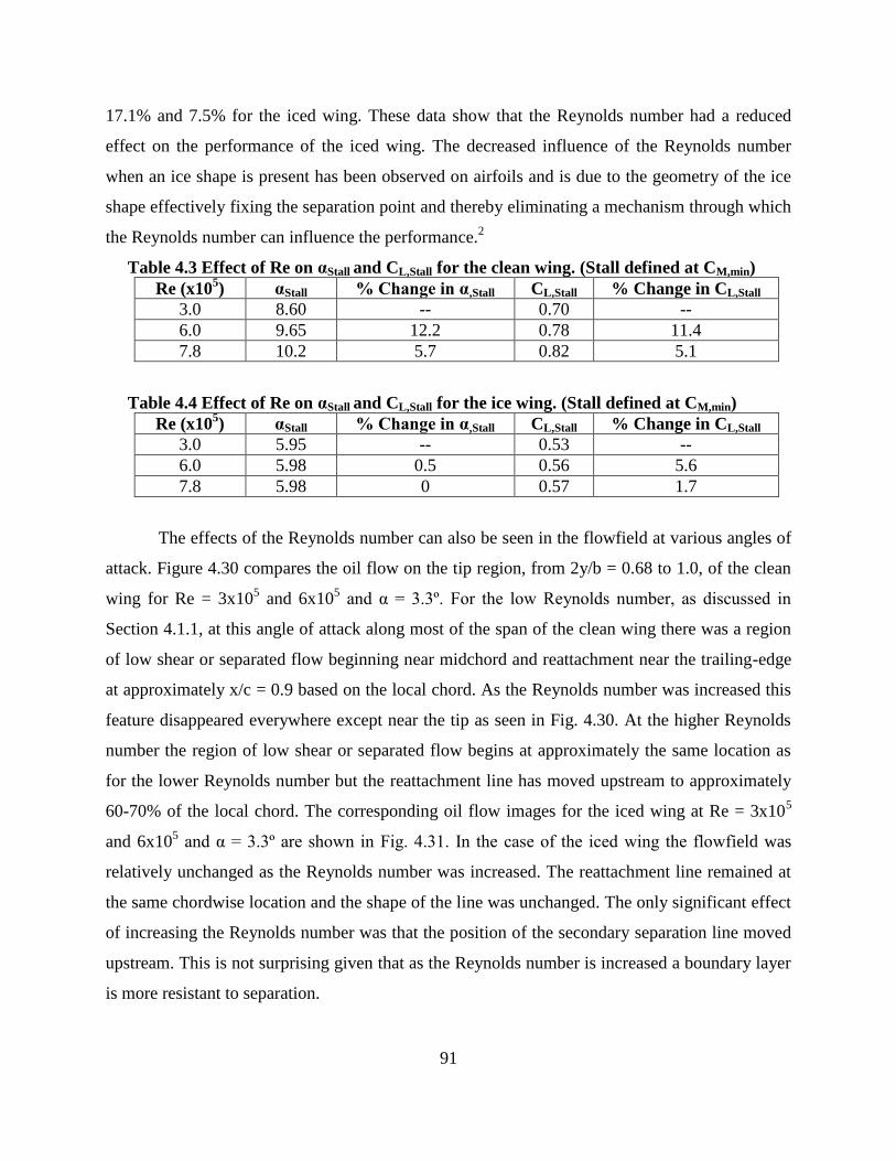
91

17.1% and 7.5% for the iced wing. These data show that the Reynolds number had a reduced

effect on the performance of the iced wing. The decreased influence of the Reynolds number

when an ice shape is present has been observed on airfoils and is due to the geometry of the ice

shape effectively fixing the separation point and thereby eliminating a mechanism through which

the Reynolds number can influence the performance.2

Table 4.3 Effect of Re on αStall and CL,Stall for the clean wing. (Stall defined at CM,min)

Re (x105) αStall % Change in α,Stall CL,Stall % Change in CL,Stall

3.0 8.60 -- 0.70 --

6.0 9.65 12.2 0.78 11.4

7.8 10.2 5.7 0.82 5.1

Table 4.4 Effect of Re on αStall and CL,Stall for the ice wing. (Stall defined at CM,min)

Re (x105) αStall % Change in α,Stall CL,Stall % Change in CL,Stall

3.0 5.95 -- 0.53 --

6.0 5.98 0.5 0.56 5.6

7.8 5.98 0 0.57 1.7

The effects of the Reynolds number can also be seen in the flowfield at various angles of

attack. Figure 4.30 compares the oil flow on the tip region, from 2y/b = 0.68 to 1.0, of the clean

wing for Re = 3x105 and 6x10

5 and α = 3.3º. For the low Reynolds number, as discussed in

Section 4.1.1, at this angle of attack along most of the span of the clean wing there was a region

of low shear or separated flow beginning near midchord and reattachment near the trailing-edge

at approximately x/c = 0.9 based on the local chord. As the Reynolds number was increased this

feature disappeared everywhere except near the tip as seen in Fig. 4.30. At the higher Reynolds

number the region of low shear or separated flow begins at approximately the same location as

for the lower Reynolds number but the reattachment line has moved upstream to approximately

60-70% of the local chord. The corresponding oil flow images for the iced wing at Re = 3x105

and 6x105 and α = 3.3º are shown in Fig. 4.31. In the case of the iced wing the flowfield was

relatively unchanged as the Reynolds number was increased. The reattachment line remained at

the same chordwise location and the shape of the line was unchanged. The only significant effect

of increasing the Reynolds number was that the position of the secondary separation line moved

upstream. This is not surprising given that as the Reynolds number is increased a boundary layer

is more resistant to separation.

92

Similar trends were observed at higher angles of attack. Figure 3.32 shows oil flow on the

clean wing, in the region from 2y/b = 0.625 to 0.925, for α = 7.6º at Reynolds numbers of 3x105

and 6x105. At the lower Reynolds number the flow separated near the leading-edge due to the

adverse pressure gradient and a small leading-edge vortex was present along nearly the entire

span. The primary separation, reattachment and secondary separation are all visible in Fig. 4.32.

At Re = 6x105 an oil accumulation line was still present indicating some separation however the

other features were not visible. While the leading-edge vortex may not have disappeared entirely

it certainly decreased in size due to the change in Reynolds number. The effect of increasing

Reynolds number on the leading-edge vortex was very similar to the effect on laminar separation

bubbles on airfoils. Oil flow images for the iced wing at the two Reynolds numbers, in the region

from 2y/b = 0.45 to 0.75, for α = 5.5º are shown in Fig. 4.33. Similar to the lower angle of attack,

the flowfield of the iced wing remained relatively unchanged as the Reynolds number was

doubled. Even in the case of a highly nonlinear reattachment line the shape and location of the

line were not altered. Similar to the lower angle of attack, the only effect of increasing the

Reynolds number was a change in the secondary separation location.

Overall, the data presented here are encouraging because they suggest that the presence

of ice reduces the effects of Reynolds number. This has important implications for the majority

of experimental work that remains to be done on swept wing icing. It should be stated, however,

that these experiments were performed at very low Reynolds number, and while the results are

encouraging, they may not necessarily hold at higher Reynolds numbers.

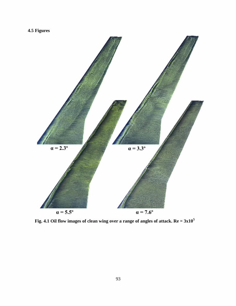
93

4.5 Figures

α = 2.3º

α = 7.6º α = 5.5º

α = 3.3º

Fig. 4.1 Oil flow images of clean wing over a range of angles of attack. Re = 3x105

94

Secondary Separation

Primary Separation

Reattachment

Fig. 4.2 Features of leading-edge vortex. Clean wing, α = 5.5º, Re = 3x105.

Fig. 4.3 Oil flow of the stalled clean wing, α =

9.6º, Re = 3x105.

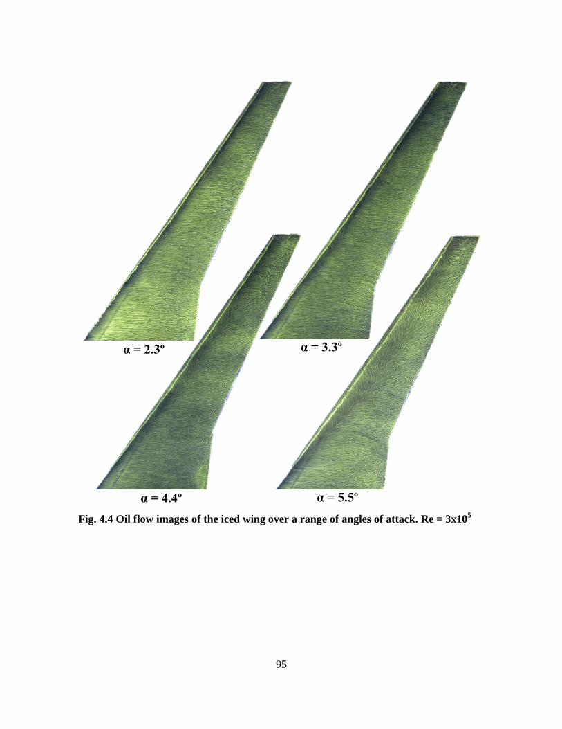
95

α = 2.3º α = 3.3º

α = 4.4º α = 5.5º

Fig. 4.4 Oil flow images of the iced wing over a range of angles of attack. Re = 3x105

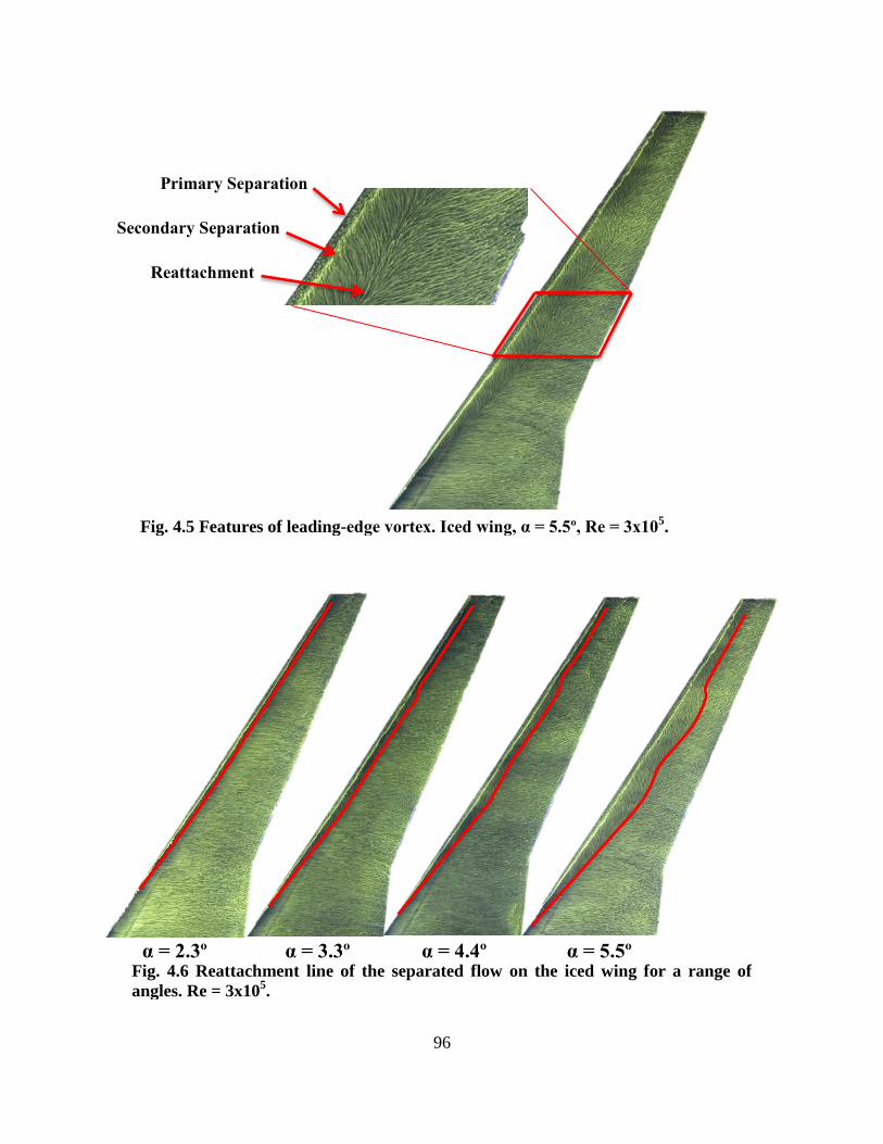
96

Primary Separation

Secondary Separation

Reattachment

Fig. 4.5 Features of leading-edge vortex. Iced wing, α = 5.5º, Re = 3x105.

α = 2.3º α = 3.3º α = 4.4º α = 5.5º Fig. 4.6 Reattachment line of the separated flow on the iced wing for a range of

angles. Re = 3x105.

97

Fig. 4.7 Oil flow of the stalled iced wing, α =

6.5º, Re = 3x105.

98

CL

-10 -5 0 5 10 15 20-0.4

-0.2

0

0.2

0.4

0.6

0.8

1

CD

-10 -5 0 5 10 15 200

0.05

0.1

0.15

0.2

0.25

0.3

CM

-10 -5 0 5 10 15 20-0.3

-0.25

-0.2

-0.15

-0.1

-0.05

0

0.05

0.1

Fig. 4.8 Force balance results for the clean and iced wing.

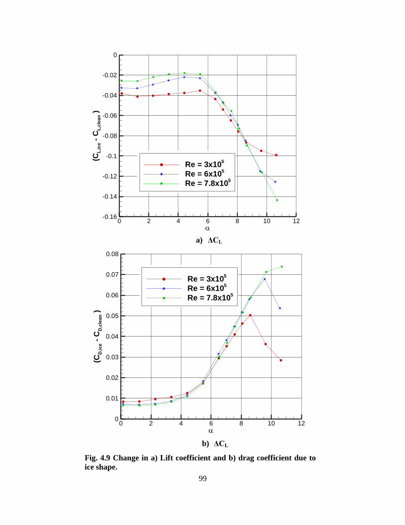
99

(CL

,ic

e-

CL

,cle

an

)

0 2 4 6 8 10 12-0.16

-0.14

-0.12

-0.1

-0.08

-0.06

-0.04

-0.02

0

(CD

,ic

e-

CD

,cle

an

)

0 2 4 6 8 10 120

0.01

0.02

0.03

0.04

0.05

0.06

0.07

0.08

b) ΔCL

a) ΔCL

(CL

,ic

e-

CL

,cle

an

)

0 2 4 6 8 10 12-0.16

-0.14

-0.12

-0.1

-0.08

-0.06

-0.04

-0.02

0

Re = 3x105

Re = 6x105

Re = 7.8x105

(CL

,ic

e-

CL

,cle

an

)

0 2 4 6 8 10 12-0.16

-0.14

-0.12

-0.1

-0.08

-0.06

-0.04

-0.02

0

Re = 3x105

Re = 6x105

Re = 7.8x105

Fig. 4.9 Change in a) Lift coefficient and b) drag coefficient due to

ice shape.

100

b) Drag Coefficient

CL

-5 0 5 10 15-0.2

0

0.2

0.4

0.6

0.8

1

Force Balance

Wake Survey

CD

-5 0 5 10 150

0.05

0.1

0.15

0.2

0.25

Force Balance

Wake Survey

a) Lift Coefficient

CD

-5 0 5 10 150

0.05

0.1

0.15

0.2

0.25

Force Balance

Wake Survey

CD

-5 0 5 10 150

0.05

0.1

0.15

0.2

0.25

Force Balance

Wake Survey

Fig. 4.10 Comparison of total lift and drag for the clean wing measured

by the force balance and by the wake survey technique. Re = 6x105

101

b) Drag Coefficient

CL

-5 0 5 10 15-0.2

0

0.2

0.4

0.6

0.8

1

Force Balance

Wake Survey

CD

-5 0 5 10 150

0.05

0.1

0.15

0.2

0.25

Force Balance

Wake Survey

a) Lift Coefficient

CD

-5 0 5 10 150

0.05

0.1

0.15

0.2

0.25

Force Balance

Wake Survey

CD

-5 0 5 10 150

0.05

0.1

0.15

0.2

0.25

Force Balance

Wake Survey

Fig. 4.11 Comparison of total lift and drag for the iced wing measured

by the force balance and by the wake survey technique. Re = 6x105

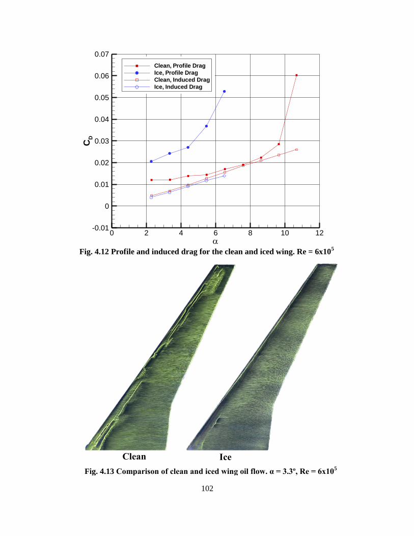
102

Clean Ice

Fig. 4.13 Comparison of clean and iced wing oil flow. α = 3.3º, Re = 6x105

Fig. 4.12 Profile and induced drag for the clean and iced wing. Re = 6x105

CD

0 2 4 6 8 10 12-0.01

0

0.01

0.02

0.03

0.04

0.05

0.06

0.07

Clean, Profile Drag

Ice, Profile Drag

Clean, Induced Drag

Ice, Induced Drag

CD

0 2 4 6 8 10 12-0.01

0

0.01

0.02

0.03

0.04

0.05

0.06

0.07

Clean, Profile Drag

Ice, Profile Drag

Clean, Induced Drag

Ice, Induced Drag

103

c) 2y/b = 0.55 d) 2y/b = 0.77

a) 2y/b = 0.11 x/c

Cp

0 0.2 0.4 0.6 0.8 1

-1.5

-1

-0.5

0

0.5

Clean

Ice

b) 2y/b = 0.36

x/c

Cp

0 0.2 0.4 0.6 0.8 1

-1.5

-1

-0.5

0

0.5

Clean

Ice

x/c

Cp

0 0.2 0.4 0.6 0.8 1

-1.5

-1

-0.5

0

0.5

Clean

Ice

x/c

Cp

0 0.2 0.4 0.6 0.8 1

-1.5

-1

-0.5

0

0.5

Clean

Ice

Fig. 4.14 Comparison of clean and iced wing CP distributions for rows 1-4. α = 3.3º,

Re = 6x105

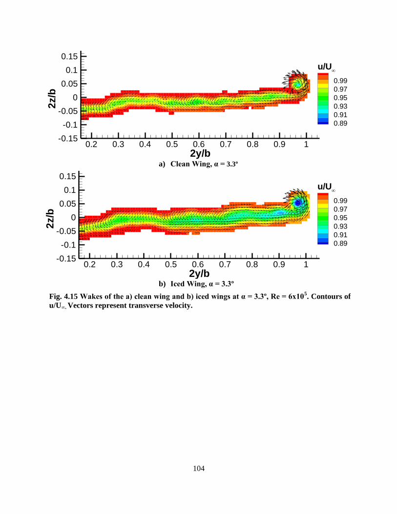
104

b) Iced Wing, α = 3.3º

a) Clean Wing, α = 3.3º

2y/b

2z/b

0.2 0.3 0.4 0.5 0.6 0.7 0.8 0.9 1-0.15

-0.1

-0.05

0

0.05

0.1

0.15

0.2

0.25

0.3

0.35

0.4

0.45

0.5

0.55

0.6

0.99

0.97

0.95

0.93

0.91

0.89

u/U

2y/b

2z/b

0.2 0.3 0.4 0.5 0.6 0.7 0.8 0.9 1-0.15

-0.1

-0.05

0

0.05

0.1

0.15

0.2

0.25

0.3

0.35

0.4

0.45

0.5

0.55

0.6

0.99

0.97

0.95

0.93

0.91

0.89

u/U

Fig. 4.15 Wakes of the a) clean wing and b) iced wings at α = 3.3º, Re = 6x105. Contours of

u/U∞. Vectors represent transverse velocity.

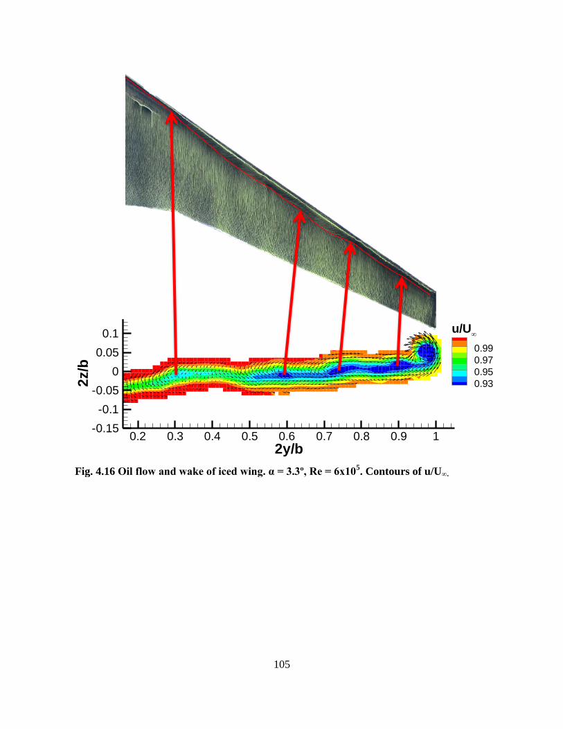
105

2y/b

2z/b

0.2 0.3 0.4 0.5 0.6 0.7 0.8 0.9 1-0.15

-0.1

-0.05

0

0.05

0.1

0.15

0.2

0.25

0.3

0.35

0.4

0.45

0.5

0.55

0.6

0.99

0.97

0.95

0.93

u/U

Fig. 4.16 Oil flow and wake of iced wing. α = 3.3º, Re = 6x105. Contours of u/U∞.

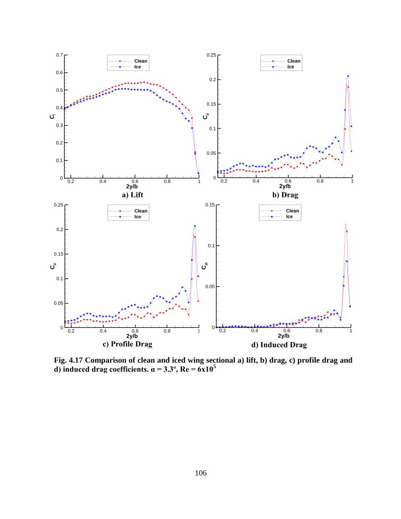
106

a) Lift b) Drag

c) Profile Drag

d) Induced Drag

2y/b

Cl

0.2 0.4 0.6 0.8 10

0.1

0.2

0.3

0.4

0.5

0.6

0.7

Clean

Ice

2y/b

Cd

0.2 0.4 0.6 0.8 10

0.05

0.1

0.15

0.2

0.25

Clean

Ice

2y/b

Cd

0.2 0.4 0.6 0.8 10

0.05

0.1

0.15

0.2

0.25

Clean

Ice

2y/b

Cd

i

0.2 0.4 0.6 0.8 10

0.05

0.1

0.15

Clean

Ice

Fig. 4.17 Comparison of clean and iced wing sectional a) lift, b) drag, c) profile drag and

d) induced drag coefficients. α = 3.3º, Re = 6x105

107

2y/b

2z/b

0.2 0.3 0.4 0.5 0.6 0.7 0.8 0.9 1-0.15

-0.1

-0.05

0

0.05

0.1

0.15

0.2

0.25

0.3

0.35

0.4

0.45

0.5

0.55

0.6

0.8

0.6

0.4

0.2

0

/max

Fig. 4.18 Contours of normalized streamwise vorticity in the wake of the iced wing. α = 3.3º, Re = 6x10

5.

Clean Ice

Fig. 4.19 Comparison of clean and iced wing oil flow. α = 5.5 º, Re = 6x105

108

x/c

Cp

0 0.2 0.4 0.6 0.8 1

-2.5

-2

-1.5

-1

-0.5

0

0.5

Clean

Ice

c) 2y/b = 0.55 x/c

Cp

0 0.2 0.4 0.6 0.8 1

-2.5

-2

-1.5

-1

-0.5

0

0.5

Clean

Ice

d) 2y/b = 0.77

x/c

Cp

0 0.2 0.4 0.6 0.8 1

-2.5

-2

-1.5

-1

-0.5

0

0.5

Clean

Ice

a) 2y/b = 0.11

x/c

Cp

0 0.2 0.4 0.6 0.8 1

-2.5

-2

-1.5

-1

-0.5

0

0.5

Clean

Ice

b) 2y/b = 0.36

Fig. 4.20 Comparison of clean and iced wing CP distributions for rows 1-4. α = 5.5º, Re

= 6x105

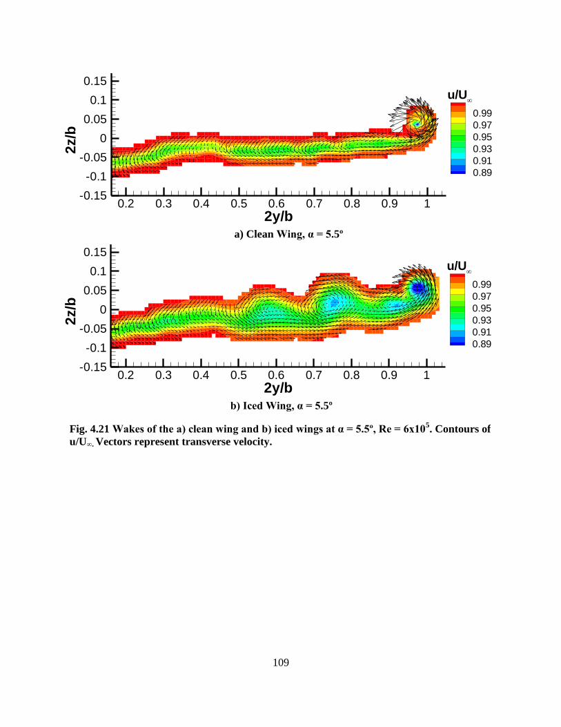
109

a) Clean Wing, α = 5.5º

b) Iced Wing, α = 5.5º

2y/b

2z/b

0.2 0.3 0.4 0.5 0.6 0.7 0.8 0.9 1-0.15

-0.1

-0.05

0

0.05

0.1

0.15

0.2

0.25

0.3

0.35

0.4

0.45

0.5

0.55

0.6

0.99

0.97

0.95

0.93

0.91

0.89

u/U

2y/b

2z/b

0.2 0.3 0.4 0.5 0.6 0.7 0.8 0.9 1-0.15

-0.1

-0.05

0

0.05

0.1

0.15

0.2

0.25

0.3

0.35

0.4

0.45

0.5

0.55

0.6

0.99

0.97

0.95

0.93

0.91

0.89

u/U

Fig. 4.21 Wakes of the a) clean wing and b) iced wings at α = 5.5º, Re = 6x105. Contours of

u/U∞. Vectors represent transverse velocity.

110

2y/b

2z/b

0.2 0.3 0.4 0.5 0.6 0.7 0.8 0.9 1-0.15

-0.1

-0.05

0

0.05

0.1

0.15

0.2

0.25

0.3

0.35

0.4

0.45

0.5

0.55

0.6

0.99

0.97

0.95

0.93

u/U

Fig. 4.22 Oil flow and wake of the iced wing at α = 5.5º and Re = 6x105. Contours of

u/U∞. Vectors represent transverse velocity. Reattachment line of the leading-edge

vortex is highlighted.

2y/b

2z/b

0.2 0.3 0.4 0.5 0.6 0.7 0.8 0.9 1-0.15

-0.1

-0.05

0

0.05

0.1

0.15

0.2

0.25

0.3

0.35

0.4

0.45

0.5

0.55

0.6

0.9

0.7

0.5

0.3

0.1

/max

Fig. 4.23 Contours of normalized streamwise vorticity in the wake of the iced wing. α

= 5.5º, Re = 6x105.

111

2y/b

Cl

0.2 0.4 0.6 0.8 10

0.1

0.2

0.3

0.4

0.5

0.6

0.7

0.8

Clean

Ice

a) Lift

2y/b

Cd

0.2 0.4 0.6 0.8 10

0.05

0.1

0.15

0.2

0.25

0.3

0.35

Clean

Ice

b) Drag

2y/b

Cd

p

0.2 0.4 0.6 0.8 10

0.05

0.1

0.15

0.2

0.25

Clean

Ice

c) Profile Drag

2y/b

Cd

i

0.2 0.4 0.6 0.8 10

0.05

0.1

0.15

0.2

0.25

Clean

Ice

d) Induced Drag

Fig. 4.24 Comparison of clean and iced wing sectional a) lift, b) drag, c) profile drag and

d) induced drag coefficients. α = 5.5º, Re = 6x105

112

Clean, α = 10.7 º Ice, α = 6.5 º

Fig. 4.25 Stalled flowfield comparison of clean and iced wing oil flow. Re =

6x105

113

c) 2y/b = 0.55 d) 2y/b = 0.77

a) 2y/b = 0.11 b) 2y/b = 0.36

x/c

Cp

0 0.2 0.4 0.6 0.8 1

-4.5

-4

-3.5

-3

-2.5

-2

-1.5

-1

-0.5

0

Clean, = 10.7 deg.

Ice, = 6.5 deg.

x/c

Cp

0 0.2 0.4 0.6 0.8 1

-4.5

-4

-3.5

-3

-2.5

-2

-1.5

-1

-0.5

0

Clean, = 10.7 deg.

Ice, = 6.5 deg.

x/c

Cp

0 0.2 0.4 0.6 0.8 1

-4.5

-4

-3.5

-3

-2.5

-2

-1.5

-1

-0.5

0

Clean, = 10.7 deg.

Ice, = 6.5 deg.

x/c

Cp

0 0.2 0.4 0.6 0.8 1

-4.5

-4

-3.5

-3

-2.5

-2

-1.5

-1

-0.5

0

Clean, = 10.7 deg.

Ice, = 6.5 deg.

Fig. 4.26 Comparison of clean and iced wing CP distributions for rows 1-4. Both wings

beyond stalling angle of attack. Clean wing α = 10.7º, Iced wing α = 6.5º, Re = 6x105

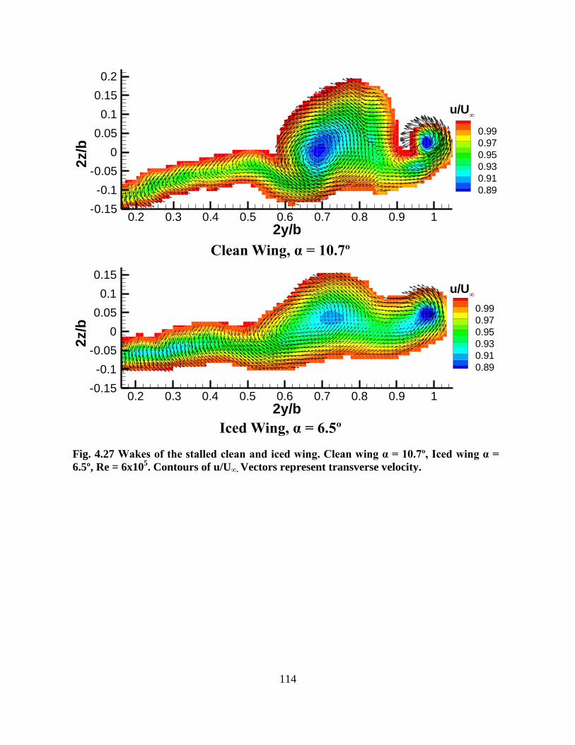
114

Clean Wing, α = 10.7º

2y/b

2z/b

0.2 0.3 0.4 0.5 0.6 0.7 0.8 0.9 1-0.15

-0.1

-0.05

0

0.05

0.1

0.15

0.2

0.25

0.3

0.35

0.4

0.45

0.5

0.55

0.6

0.99

0.97

0.95

0.93

0.91

0.89

u/U

Iced Wing, α = 6.5º

2y/b

2z/b

0.2 0.3 0.4 0.5 0.6 0.7 0.8 0.9 1-0.15

-0.1

-0.05

0

0.05

0.1

0.15

0.2

0.25

0.3

0.35

0.4

0.45

0.5

0.55

0.6

0.99

0.97

0.95

0.93

0.91

0.89

u/U

Fig. 4.27 Wakes of the stalled clean and iced wing. Clean wing α = 10.7º, Iced wing α =

6.5º, Re = 6x105. Contours of u/U∞. Vectors represent transverse velocity.

115

2y/b

Cl

0.2 0.4 0.6 0.8 10

0.1

0.2

0.3

0.4

0.5

0.6

0.7

0.8

0.9

1

1.1

1.2 Clean, = 10.7 deg.

Ice, = 6.5 deg.

2y/b

Cd

0.2 0.4 0.6 0.8 10

0.05

0.1

0.15

0.2

0.25

0.3

0.35

0.4

0.45

0.5

0.55

0.6

Clean, = 10.7 deg.

Ice, = 6.5 deg.

2y/b

Cd

p

0.2 0.4 0.6 0.8 10

0.05

0.1

0.15

0.2

0.25

0.3

Clean, = 10.7 deg.

Ice, = 6.5 deg.

2y/b

Cd

i

0.2 0.4 0.6 0.8 1-0.1

-0.05

0

0.05

0.1

0.15

0.2

0.25

0.3

0.35

Clean, = 10.7 deg.

Ice, = 6.5 deg.

a) Lift b) Drag

c) Profile Drag

d) Induced Drag

Fig. 4.28 Comparison of stalled clean and iced wing sectional a) lift, b) drag, c) profile

drag and d) induced drag coefficients. Clean wing α = 10.7º, Iced wing α = 6.5º, Re =

6x105.

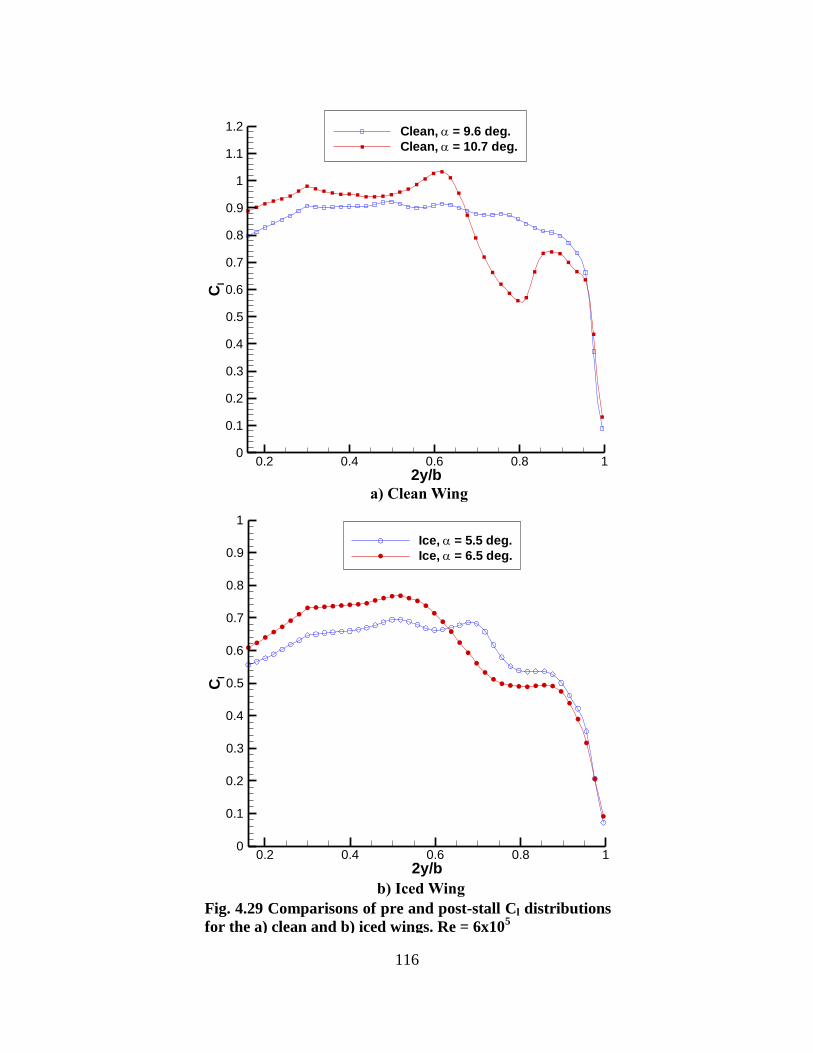
116

2y/b

Cl

0.2 0.4 0.6 0.8 10

0.1

0.2

0.3

0.4

0.5

0.6

0.7

0.8

0.9

1

1.1

1.2 Clean, = 9.6 deg.

Clean, = 10.7 deg.

2y/b

Cl

0.2 0.4 0.6 0.8 10

0.1

0.2

0.3

0.4

0.5

0.6

0.7

0.8

0.9

1

Ice, = 5.5 deg.

Ice, = 6.5 deg.

a) Clean Wing

b) Iced Wing

Fig. 4.29 Comparisons of pre and post-stall Cl distributions

for the a) clean and b) iced wings. Re = 6x105

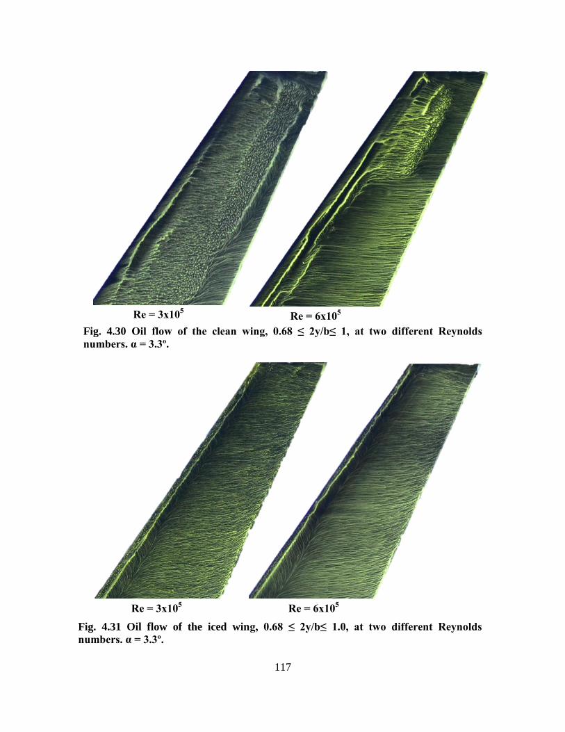
117

Re = 6x105

Re = 3x105

Fig. 4.30 Oil flow of the clean wing, 0.68 ≤ 2y/b≤ 1, at two different Reynolds

numbers. α = 3.3º.

Re = 6x105

Re = 3x105

Fig. 4.31 Oil flow of the iced wing, 0.68 ≤ 2y/b≤ 1.0, at two different Reynolds

numbers. α = 3.3º.

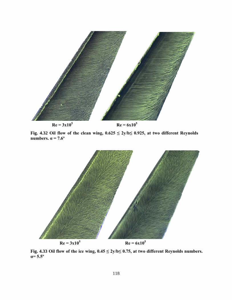
118

Re = 6x105

Re = 3x105

Fig. 4.32 Oil flow of the clean wing, 0.625 ≤ 2y/b≤ 0.925, at two different Reynolds

numbers. α = 7.6º

Re = 6x105

Re = 3x105

Fig. 4.33 Oil flow of the ice wing, 0.45 ≤ 2y/b≤ 0.75, at two different Reynolds numbers.

α= 5.5º

119

Chapter 5

Conclusions and Recommendations

5.1 Conclusions

The purpose of this work was to demonstrate the use of various experimental techniques

applied to understanding the aerodynamics of a swept wing with ice. While the tests were

performed at low Reynolds, and are not directly applicable to flight, the results show that a great

deal can be learned by applying the techniques discussed above. Several observations and

conclusions from this work were:

1. The clean wing flowfield was typical of swept wings at low Reynolds numbers.

a. The oil flow showed a small region of separated flow near the leading-edge due to

the adverse pressure gradient seen in the surface pressure distributions.

b. The lift coefficient distribution showed that the outboard sections were heavily

loaded compared to the inboard sections.

c. The amount of spanwise flow increased with angle of attack.

d. The structure of the wake was relatively unchanged as the angle of attack

increased prior to stall.

e. The stalled flowfield was dominated by a part-span leading-edge vortex that

formed just inboard of midspan. The leading-edge vortex was shed into the wake

at approximately 60-70% span.

2. The iced wing flowfield was significantly different from the clean wing.

a. Beginning at low angles of attack, a leading-edge vortex formed along most of the

span as a result of flow separation from the tip of the ice shape.

b. The flowfield of the leading-edge vortex was consistent with previous

observations by Poll18

on swept wings with sharp leading-edges, by Broeren46

and

Khodadoust7 on swept wings with iced leading-edges and the computational

results of Kwon and Sankar30

for a swept wing with an iced leading-edge.

c. The size of the leading-edge vortex increased with the angle of attack.

120

d. The leading-edge vortex flowfield was similar to the recirculation bubble

flowfield behind a horn ice shape on an airfoil, but there were several important

differences due to the three-dimensional nature of the vortex.

e. In general, the size of the vortex relative to the local chord increased as the tip

was approached.

f. As the angle of attack increased significant spanwise variation in the leading-edge

vortex began to form as several kinks began to develop in the reattachment line.

g. The iced wing stalled when the flow failed to reattach over the outboard sections.

Similar to the clean wing case, the leading-edge vortex was shed into the wake

inboard of the tip.

3. The ice shape had a significant effect on the performance of the wing.

a. The force balance data showed an increase in the minimum drag coefficient of

78.8%, a decrease in the stalling angle of attack of 3.5º and a decrease in CL,Stall of

38.4%. The ice shape also increased the pitching moment.

b. The 5-hole probe results showed that the ice shape significantly increased the

profile drag but the induced drag was relatively unaffected. Increased pressure

drag due to the separated flowfield was responsible for the increased profile drag.

c. The balance data showed that as the wing stalled the pitching moment increased,

indicating tip stall. This was confirmed by the oil flow images which showed

separated flow on the outboard sections of the wing, while the inboard sections

remained attached.

4. The spanwise distributions of lift and drag offered insight into the aerodynamics that

could not be obtained only with the use of balance measurements.

a. The distributions of lift and drag showed that the ice shape had the largest impact

on the sectional aerodynamics on the outboard sections of the wing. This was

consistent with the oil flow which showed the leading-edge vortex on the iced

wing was generally larger relative to the local chord on the outboard sections.

b. As the wing stalled, the sectional lift coefficients decreased on the outboard

sections of the wing but the lift continued to increase inboard of the leading-edge

vortex. Due to the sweep of the wing this change in the spanwise lift distribution

shifted the center of pressure of the wing forward increasing the pitching moment.

121

c. The flow remained attached and the lift continued to increase on the inboard

sections. This compensated for the loss of lift on the outboard sections preventing

the lift of the wing from dropping dramatically at stall.

d. It was shown that the kinks in the reattachment line observed in the oil flow on

the iced wing, corresponded to localized regions of large axial velocity deficit and

streamwise vorticity concentrations in the wake.

e. The spanwise distributions of drag showed that these kinks also corresponded to

peaks in the sectional profile and induced drag.

5. Finally, it was observed that the ice shape reduced the influence of the Reynolds number.

a. Doubling the Reynolds number, from 3x106 to 6x10

6, resulted in an increase in

CL,Stall of 11.4% for the clean wing, but only 5.6% for the iced wing.

b. For the same change in Reynolds number, significant changes in the flowfield of

the clean wing were observed at various angles of attack; however, the changes in

the iced wing flowfield were generally insignificant.

c. The trend of decreased Reynolds number effects due to ice has been observed on

airfoils in the past.

d. These results are encouraging, but these tests were performed at very low

Reynolds numbers and this result may not hold for higher Reynolds number.

5.2 Recommendations

The work presented in this thesis is far from complete. The following is a list of

recommendations on how to improve and expand upon this work.

1. First and foremost, the quality of the model must be improved. At the time of this

writing, work is underway to improve the surface which will allow for higher quality

clean wing data.

2. The 5-hole probe wake surveys provide a wealth of information but there is significant

room for improvement. There are several ways in which these results may possibly be

improved.

a. A calibration with finer resolution may improve the results.

122

b. When acquiring data, the results may be improved by using smaller stepsizes

when traversing the probe, particularly near the tip vortex where velocity

gradients are largest.

c. It would be beneficial to improve the data reduction techniques. This includes

the local interpolation method used to apply the calibration and the method used

to solve the Poisson equation for the stream function.

d. A method of properly handling the boundary condition on the inboard edge of

the measurement plane when solving the Poisson equation for the stream

function is needed.

e. The inboard edge of the measurement plane should be extended closer to the

root.

f. Performing wake surveys at several streamwise locations would provide

information about the evolution of the wake and how the ice effects its growth.

g. Wake surveys should be performed over a wider range of angles of attack and

Reynolds number.

3. Off-body flowfield measurements, such as PIV, would be extremely beneficial for

trying to understand the aerodynamics of this swept wing with ice. These measurements

could be used to more thoroughly investigate the leading-edge vortex behind the ice

shape, and answer questions such as what causes the kinks in the reattachment line.

4. Different ice shapes should be tested to see if there is a significant difference in the

performance at this low Reynolds number. This information would be useful for future

small scale wind tunnel testing.

123

Appendix A

Five-Hole Probe Calibration

In order to extract information such as lift and drag from the wake of a finite wing it is

necessary to measure all three components of velocity as well as total and static pressure. A five-

hole probe (5HP) is capable of measuring all of these quantities simultaneously. This appendix

will describe the theory of operation, calibration setup and calibration procedure for the 5HP

used in this study.

A. 1 Theory of Operation

The probe used in this study was an Aeroprobe Corp., model PS5-C318-152 five-hole

probe. The tip of the probe was conical with a base diameter of 0.125-ines. The probe tip

contained a central port and four peripheral ports. In order to calibrate the probe for flow

angularity it was necessary to develop a relationship between the five measured pressures and the

flow angle. This was accomplished by placing the probe in a uniform flow and rotating the probe

with respect to the flow.

The pressure ports were labeled 1-5, see Fig. A.1 for the hole numbering convection, and

the probe coordinate system was defined as shown in Fig. A.2. While the axes of the probe

coordinate system correspond to the wing coordinate axes the pitch and yaw angles ( , ) are

different from the wing pitch and yaw coefficients ( , ). The relation between the two sets of

angles was given by:

(A.1)

(A.2)

The reason for this difference was that the definitions of the pitch and yaw angles for the probe

shown in Fig. A.2 were more convenient during calibration.

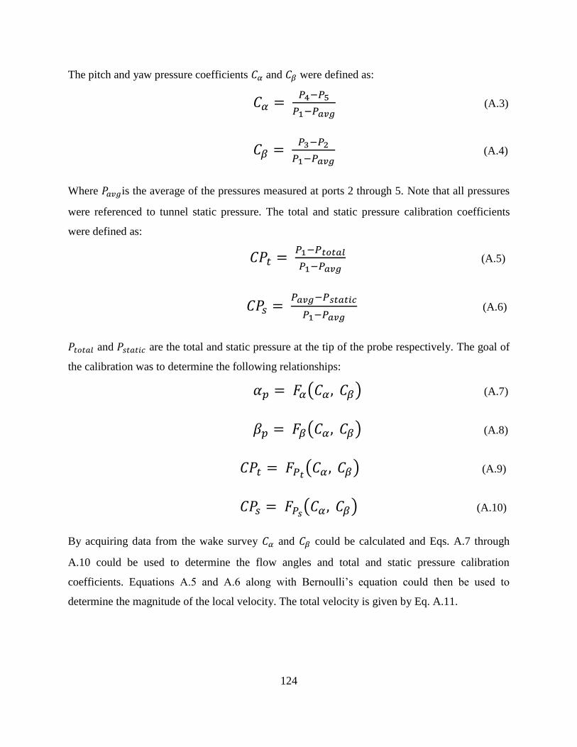
124

The pitch and yaw pressure coefficients and were defined as:

(A.3)

(A.4)

Where is the average of the pressures measured at ports 2 through 5. Note that all pressures

were referenced to tunnel static pressure. The total and static pressure calibration coefficients

were defined as:

(A.5)

(A.6)

and are the total and static pressure at the tip of the probe respectively. The goal of

the calibration was to determine the following relationships:

( ) (A.7)

( ) (A.8)

( ) (A.9)

( ) (A.10)

By acquiring data from the wake survey and could be calculated and Eqs. A.7 through

A.10 could be used to determine the flow angles and total and static pressure calibration

coefficients. Equations A.5 and A.6 along with Bernoulli’s equation could then be used to

determine the magnitude of the local velocity. The total velocity is given by Eq. A.11.

125

√

⁄ ( )( ) (A.11)

The pitch and yaw angles, determined from Eqs. A.7 and A.8, in the probe coordinate system

( , ) were then be converted to the wing coordinate system using Eqs. A.1 and A.2 and the

velocity components were calculated.

( ) ( ) (A.12)

( ) (A.13)

( ) ( ) (A.14)

Where is in the streamwise direction, is along the span of the wing positive towards the tip

and positive points from the lower surface to the upper surface of the wing. In addition, the

total and static pressure coefficients could be calculated be solving Eqs. A.5 and A.6 for the total

and static pressure respectively and then non-dimensionalizing by the freestream dynamic

pressure.

( )

(A.15)

( )

(A.16)

Unlike the total and static pressure calibration coefficients, Eqs. A. 15 and 16 are the actual total

and static pressure coefficients. Before any wake survey could be completed it was necessary to

determine the relations given by Eqs. A.7 through A.10. These relationships were obtained

through a calibration that consisted of acquiring pressure data over a range of flow conditions.

The calibration setup, procedure and results will be now be discussed.

126

A. 2 Experimental Setup

In Fig. A.2 there are two sets of angles defined. The pitch and yaw angles ( , ) and

the cone and roll angles ( , ). When calibrating the probe it is necessary to rotate the probe

throughout a range of angles in a uniform flow, and it is important that the tip of the probe

remain in the same location so as not to be affected by freestream non-uniformities. The

calibration discussed here was carried out in the 3x4 Low Speed Wind Tunnel described in

Section 3.1.1. Inside this tunnel it was significantly easier to rotate the probe through the cone

and roll angles as opposed to pitch and yaw. The relationship between the two sets of angles is

given by Eqs. A.17 and A.18.

( ) ( ) ( ) (A.17)

( ) ( ) ( ) (A.18)

Therefore, rotating the probe through a series of cone and roll angles was equivalent to rotating

the probe through pitch and yaw angles.

The setup used to mount the probe in the wind tunnel is shown in Fig. A.3. The entire

probe support system was mounted to the tunnel turntable used to control the model angle of

attack, and was positioned so that the probe tip was at the center of the turntable. The turntable

was used to control the cone angle ( ) of the probe. The probe support structure was placed far

enough downstream of the probe tip so as to not interfere with the flow. The probe support

structure consists of several components. The base of the probe support was an aluminum rod 2

inches in diameter that was machined at the top, see Fig. A.4. Note that in Fig. A.4 the support

was not mounted in the same location as shown in Fig. A.3. During the first iteration the support

structure was mounted as shown in Fig. A.4 and there were significant interference effects at the

tip of the probe due to the large size of the support structure. The final calibration was performed

with probe mounted as shown in Fig. A.3. While the tunnel turntable was used to automatically

control the cone angle ( ), the roll angle ( ) was controlled manually via a small rotation stage

mounted to the base of the support, see Fig. A.5. This rotation stage could be used to accurately

set the roll angle between 0º and 359º. An adaption plate was mounted to the rotation stage and

the probe holder was mounted to the adaptation plate as shown in Fig. A.6. The probe was placed

into a slot in the probe holder and held in place with two set screws as shown in Fig. A.7. As can

127

be seen in Fig. A.3 through Fig. A.7 the probe support system was designed to allow the pressure

lines pass through adaption plate, rotation stage and the base. The lines then ran down the

backside of the base and through the tunnel floor. These lines were then connected to the second

± 0.35 psid module described in Section 3.1.3.2.

Recall that the total and static pressure coefficients and , given by Eqs. A.5 and

A.6, required the total and static pressure respectively, however during calibration neither of

these pressures were measured directly. During calibration the total pressure at the tip of the

probe was the tunnel total pressure. In Eq. A.5, if were measured directly it would have

been referenced to tunnel static pressure giving . Therefore, during calibration the total

pressure coefficient was calculated using Eq. A.19.

(A.19)

Similarly for the static pressure coefficient, if were measured directly it would have been

referenced to tunnel static pressure. But during calibration at the probe tip is the tunnel

static pressure, and therefore the static pressure coefficient was calculated using:

(A.20)

A. 3 Procedure

Using the tunnel turntable the cone angle was varied from -24º to 24º. The angle

calibration was divided into three regions each with a different stepsize. Table A.1 lists the

regions and the corresponding stepsizes.

Table A.1 Cone angle stepsizes.

Cone Angle Region ( ) Stepsize ( )

| | | | | |

Using the manual rotation stage the roll angle ( ) was varied from 0º to 171º in

increments of 9º. These ranges of cone and roll angles effectively calibrated the probe for any

velocity vector within a cone with a half angle of 24º. In addition to calibrating the probe over a

128

range of angles it was also necessary to calibrate over a range of speeds. This was due to the

influence of Reynolds number, especially at higher incoming flow angles when the flow begins

to separate from the downstream face of the probe.48

Table A.2 lists the Reynolds numbers based

on probe tip diameter, and the corresponding Reynolds number based on the swept wing model

mean aerodynamic chord, at which the probe was calibrated.

Table A.2 Reynolds numbers for five-hole probe calibration

Re Based on Probe Tip (Rep) Re Based on Model Cmac

2690 1.5x105

5381 3x105

8071 4.5x105

10762 6x105

Note that the probe was not calibrated at the highest Reynolds number of 7.8x105 based on the

model mean aerodynamic chord. This was due to considerations based on time and experimental

uncertainty. At the maximum tunnel speed the dynamic pressure in the test section exceeds 0.35

psi and calibrating at that speed would have required the use of a ± 1 psid module. This would

have resulted in higher uncertainty at the lower speeds. Due to time constraints it was not

feasible to perform a separate calibration for the higher speed.

Due to the use of the manual rotation stage for changing the roll angle the calibration

process was not fully automated. All automated portions of the process were controlled through

LabVIEW. The calibration procedure was as follows.

1. Specify the cone angles and speed.

2. Input the roll angle and start the tunnel.

3. The LabVIEW program then stepped the probe through all of the specified cone

angles, recording the 5HP pressures and tunnel conditions at each point.

4. After stepping through all of the cone angles the tunnel speed was changed to the

next specified speed.

5. Repeat steps 3 and 4 for all of the desired speeds.

6. The tunnel then shut off and the roll angle was manually adjusted.

7. Repeat steps 2-6 for all roll angles.

129

A. 4 Calibration Results

The calibration surfaces for , , and at a Reynolds number based on probe tip

diameter of 10762 are shown in Figs. A.9 through A.12 respectively. Notice that the surfaces for

and are very similar to each other, only rotated 90º. This was due to the symmetry of the

probe, if the probe were perfectly symmetrical it would be expected that these contour plots

would be identical except for the rotation. If the probe were symmetrical it would also be

expected that the contour plots of and would have symmetry about the and

axes, however as seen from Figs. A.11 and A.12 this is not quite the case. Each contour

plot appears nearly symmetrical but shifted slightly. The static pressure coefficient shows

considerable deviation from symmetry when both and are negative. The reason for the

asymmetries of these plots is slight manufacturing defects in the probe and possible tunnel

freestream non-uniformities if the probe tip did not stay in exactly the same location through the

calibration.

These calibration surfaces were used to determine the flow angles and the total and static

pressure coefficients from data acquired during a wake survey. This was accomplished using

Matlab’s built in TriScatteredInterp function. This function constructs an interpolating surface

consisting of a mesh made up of triangular elements. This interpolating surface served as the

desired relationships defined in Eqs. A7 through A.10. In order to determine the value of the

surface at a given point the interpolating function created by TriScatteredInterp was called and a

local linear interpolation was performed.

The accuracy of this method was assessed by taking additional measurements in the

calibration setup that were not used in creating the calibration surfaces. This provided a set of

data at known conditions. The pressures measured by the 5HP were used to calculate and

which were then input into the interpolating functions and values of , , and were

determined. The differences between the actual flow angles and the measured flow angles

determined from the calibration surfaces are plotted in Fig. A.12 against √

which is a measure of the total flow angle. The probe Reynolds number was 10762. The

subscript ‘actual’ indicates that this value was known, not determined from the calibration. It can

be seen that the difference between the measured and actual flow angle is within ±0.10º over

most of the calibration range. The scatter increases as the flow angularity increases, but the

130

largest differences occurred at very small angles. The largest difference between actual and

predicted flow angles occurring at small angles was observed for all Reynolds number and was

due to irregularities in the calibration surface at small angles. The reason for these irregularities

are unknown, but it was determined that the error caused by this problem was negligible since it

only affected small angles that do not contribute significantly to the various quantities of interest.

In Fig. A.13 the difference between the measured and actual total and static pressure calibration

coefficients are plotted against the total flow angularity. A trend of increasing difference and

scatter is seen as the flow angularity increases. Table A.3 lists the root mean square error

of , , and determined from applying the calibration generated at a given Reynolds

number to data taken at the corresponding Reynolds number with known flow angles. The

average error in across all of the Reynolds numbers is 0.167º with a standard deviation of

0.0221º. The average error in is slightly less at 0.139º across all Reynolds however the

standard deviation is greater at 0.0425º. From Fig. A.12 the difference between the actual and

measured flow angles is relatively constant over the range of angles implying that the percent

error is significantly higher for the lower angles. Also shown in the table is the error in velocity

at the different Reynolds number. In all cases the error is very small.

Table A.3 Root mean square error of variables determined from calibration at different

Reynolds numbers.

Rep = 2690 Rep = 5381 Rep = 8071 Rep = 10762

0.159º 0.199º 0.154º 0.155º

0.107º 0.186º 0.099º 0.163º

0.0083 0.0036 0.0028 0.0030

0.0069 0.0025 0.0019 0.0020

(ft/s) 0.0693 0.0704 0.0723 0.139

Finally, the measurements taken at known flow conditions were used to assess the effect of

Reynolds number on the calibration and data reduction by reducing data measured at one

Reynolds number using the calibration formed at a different Reynolds number. In Fig. A.14, the

difference between the measured and actual flow angles are shown for data taken at Rep = 5381

and reduced with a calibration generated at Rep = 10762. Comparing Fig. A.14 to Fig. A.12 it

can be seen that the error and the scatter increases significantly as a result of using a calibration

131

generated at a different Reynolds number. The root mean square error of and are 0.278º

and 0.360º respectively. The root mean square error of the velocity in this case increased to 1.198

ft/s. These results demonstrate the importance of calibrating the probe over a range of Reynolds

numbers.

132

A. 5 Figures

Fig. A.1 Pressure port numbering convention

Fig. A.2 Probe coordinate system and flow angle definition.

133

Fig. A.3 Probe mounted in the tunnel during calibration.

Fig. A.4 Aluminum rod used as base of

the probe support.

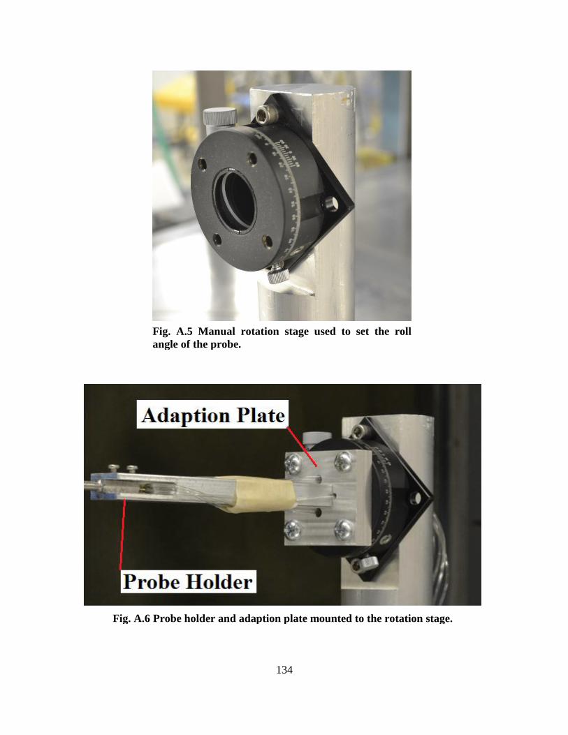
134

Fig. A.5 Manual rotation stage used to set the roll

angle of the probe.

Fig. A.6 Probe holder and adaption plate mounted to the rotation stage.

135

Fig. A.7 Probe mounted in probe holder.

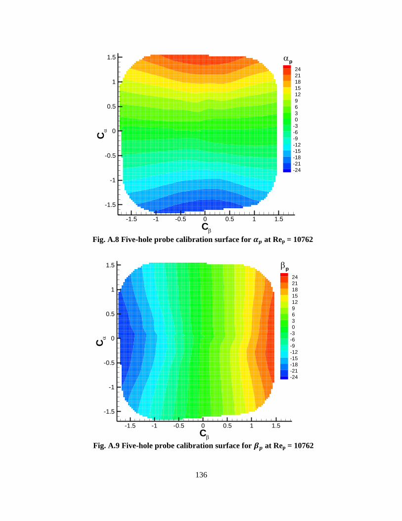
136

Fig. A.8 Five-hole probe calibration surface for 𝜶𝒑 at Rep = 10762

C

C

-1.5 -1 -0.5 0 0.5 1 1.5

-1.5

-1

-0.5

0

0.5

1

1.5

24

21

18

15

12

9

6

3

0

-3

-6

-9

-12

-15

-18

-21

-24

p

Fig. A.9 Five-hole probe calibration surface for 𝜷𝒑 at Rep = 10762

C

C

-1.5 -1 -0.5 0 0.5 1 1.5

-1.5

-1

-0.5

0

0.5

1

1.5

24

21

18

15

12

9

6

3

0

-3

-6

-9

-12

-15

-18

-21

-24

p

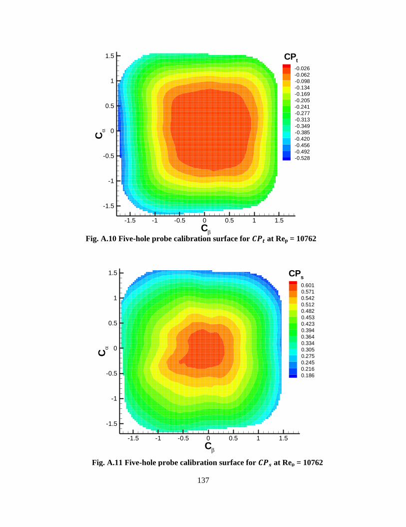
137

Fig. A.10 Five-hole probe calibration surface for 𝑪𝑷𝒕 at Rep = 10762

C

C

-1.5 -1 -0.5 0 0.5 1 1.5

-1.5

-1

-0.5

0

0.5

1

1.5

-0.026

-0.062

-0.098

-0.134

-0.169

-0.205

-0.241

-0.277

-0.313

-0.349

-0.385

-0.420

-0.456

-0.492

-0.528

CPt

Fig. A.11 Five-hole probe calibration surface for 𝑪𝑷𝒔 at Rep = 10762

C

C

-1.5 -1 -0.5 0 0.5 1 1.5

-1.5

-1

-0.5

0

0.5

1

1.5

0.601

0.571

0.542

0.512

0.482

0.453

0.423

0.394

0.364

0.334

0.305

0.275

0.245

0.216

0.186

CPs

138

Fig. A.12 Difference between actual flow angles and angles

determined from calibration surfaces. Rep = 10762

( 2

p,actual+

2

p,actual)1/2

Dif

fere

nc

e(d

eg

.)

0 5 10 15 20 25-0.4

-0.2

0

0.2

0.4

0.6

0.8

(p,actual

- p,cal

)

(p,actual

- p,cal

)

Fig. A.13 Difference between actual pressure coefficients and

those determined from calibration surfaces. Rep = 10762

( 2

p,actual+

2

p,actual)1/2

Dif

fere

nc

e

0 5 10 15 20 25-0.004

-0.002

0

0.002

0.004

0.006

0.008

(CPt,actual

- CPt,cal

)

(CPs,actual

- CPs,cal

)

139

Fig. A.14 Difference between actual and measured flow angles.

Measurements taken at Rep = 5381, calibration Rep = 10762

( 2

p,actual+

2

p,actual)1/2

Dif

fere

nc

e(d

eg

.)

0 5 10 15 20 25-0.4

-0.2

0

0.2

0.4

0.6

0.8

( 2

p,actual+

2

p,actual)1/2

Dif

fere

nc

e(d

eg

.)

0 5 10 15 20 25-0.4

-0.2

0

0.2

0.4

0.6

0.8

(p,actual

- p,cal

)

(p,actual

- p,cal

)

140

Appendix B

Derivation of the Wake Survey Equations

This appendix provides a detailed derivation of the equations used for calculating the lift

and the drag from wake survey measurements.

B. 1 Drag

Wake survey expressions can be derived by considering the control volume shown in Fig.

B.1 and making the following assumptions.

1. The upstream plane (S1) is located far enough upstream so as not to be influenced

by the model.

2. Wake survey data are measured at a single transverse plane (S2).

3. The flow at the wake survey is steady and incompressible.

4. No suction or blowing through the walls.

5. The tunnel has a uniform effective cross section

6. Turbulent stresses are negligible

A control volume analysis yields the following expression for drag.

∬ ( )

∬ ( )

(B.1)

The total pressure is defined as:

( ) (B.2)

Where U represents U∞ at S1 and u at S2. Invoking the first assumption from above and

substituting Eq. B.2 into B.1 yields:

∬ ( )

∬ (

)

(B.3)

In Eq. B.3 the first integral is only performed over the viscous wake (W) because . The

goal now is to manipulate the second integral so that it is also only over the wake region as

141

opposed to the entire downstream plane S2. By confining the integrals to the viscous wake region

the amount of data required, and therefore the survey time, is significantly reduced. In addition to

the goal of reducing the survey area it is also desired to derive separate expressions for the

profile and induced drag. Betz34

originally developed a wake integral expression for profile drag

in the absence of tunnel walls and Maskell35

extended Betz’s work to include tunnel walls. The

analysis begins by first defining the artificial velocity and the perturbation velocity .

⁄ ( ) (B.4)

(B.5)

Outside of the wake the artificial velocity is equal to the freestream velocity and the perturbation

velocity is zero. The axial velocity can be rewritten in terms of , and .

(B.6)

Note that using Eq. B.5 it can easily be shown that the last five terms of Eq. B.6 cancel resulting

in . Integrating Eq. B.6 over the downstream plane S2:

∬

∬ (

)

(B.7)

The fourth term on the right hand side of Eq. B.7 can be rewritten:

∬ ( )

∬

= ∬

(B.8)

For the first step of Eq. B.8 the factor of was taken outside of the integral because is

constant. If the area of the S2 plane is equal to the area of the upstream plane S1 then

∬ ∬

since is constant. Then the second equality of Eq. B.8 results

from conservation of mass multiplied by a factor of . Substituting Eq. B.8 into Eq. B7 and

rewriting slightly results in:

∬

∬ ( )

∬

∬

(B.9)

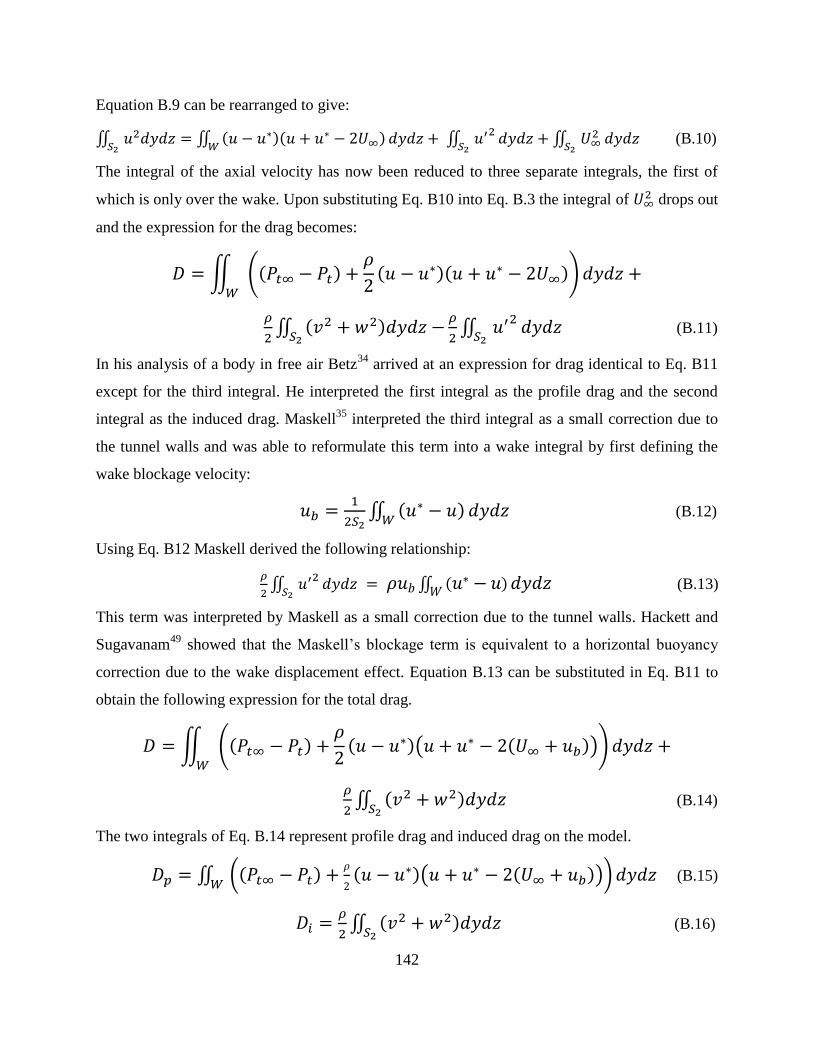
142

Equation B.9 can be rearranged to give:

∬

∬ ( )( )

∬

∬

(B.10)

The integral of the axial velocity has now been reduced to three separate integrals, the first of

which is only over the wake. Upon substituting Eq. B10 into Eq. B.3 the integral of drops out

and the expression for the drag becomes:

∬ (( )

( )( ))

∬ ( )

∬

(B.11)

In his analysis of a body in free air Betz34

arrived at an expression for drag identical to Eq. B11

except for the third integral. He interpreted the first integral as the profile drag and the second

integral as the induced drag. Maskell35

interpreted the third integral as a small correction due to

the tunnel walls and was able to reformulate this term into a wake integral by first defining the

wake blockage velocity:

∬ ( )

(B.12)

Using Eq. B12 Maskell derived the following relationship:

∬

∬ ( )

(B.13)

This term was interpreted by Maskell as a small correction due to the tunnel walls. Hackett and

Sugavanam49

showed that the Maskell’s blockage term is equivalent to a horizontal buoyancy

correction due to the wake displacement effect. Equation B.13 can be substituted in Eq. B11 to

obtain the following expression for the total drag.

∬ (( )

( )( ( )))

∬ ( )

(B.14)

The two integrals of Eq. B.14 represent profile drag and induced drag on the model.

∬ (( )

( )( ( )))

(B.15)

∬ ( )

(B.16)

143

Equation B.15 requires the integral to be performed only over viscous wake region and

was used in this study to determine the profile drag of the model. Equation B.16 still requires

measurements throughout the entire downstream plane. However, as Maskell35

showed, it is also

possible to express the induced drag in terms of a wake integral.

The streamwise vorticity and the crossflow divergence or source term are defined by

Eqs. B.17 and B.18.

(B.17)

(B.18)

The transverse stream function and velocity potential are defined by Eqs. B.19 and B.20.

(B.19)

(B.20)

These differential equations are subject to the following boundary conditions applied on the

tunnel walls (the boundary of S2).

(B.21)

(B.22)

The first boundary condition is the result of requiring the tunnel wall to be a streamline and the

second boundary condition results from requiring no flow normal to the tunnel wall. Equations

B.19 and B.20 are satisfied if:

(B.22)

(B.23)

Equations B.22 and B.23 can be substituted into Eq. B.16 to give:

∬ ( )

∬ ( (

) (

))

(B.24)

The right hand side can be rearranged slightly to give:

∬ ( )

∬ ((

) (

))

(B.25)

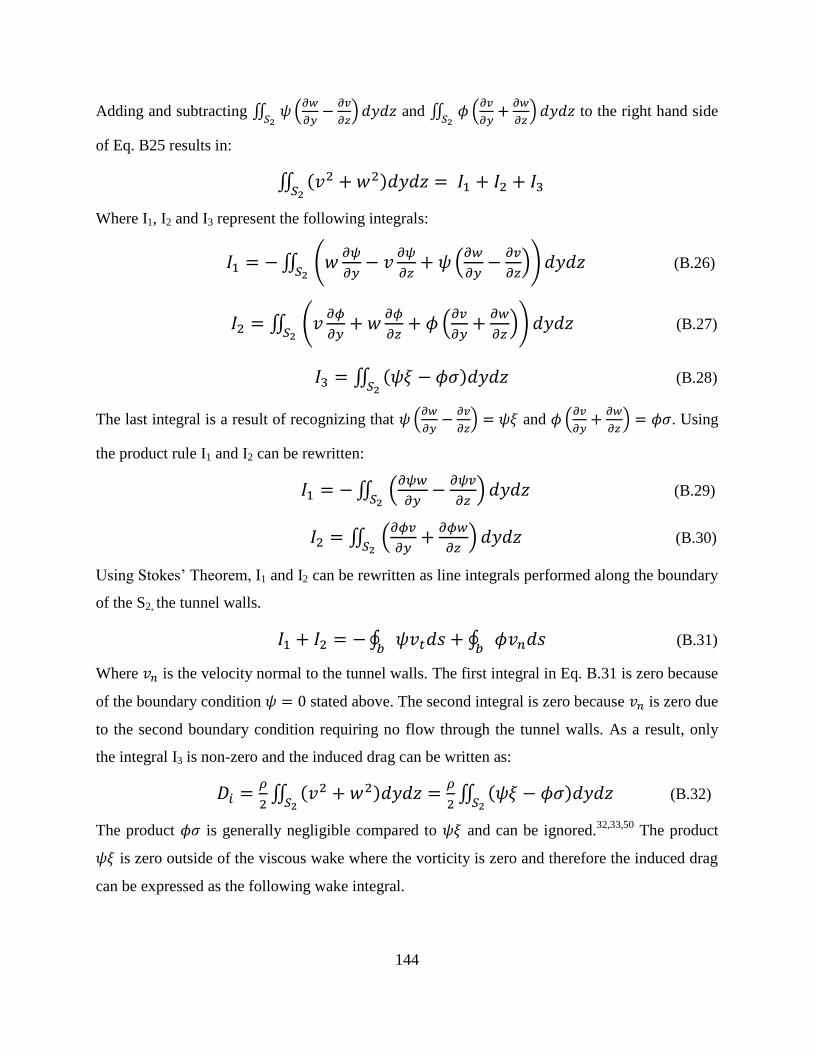
144

Adding and subtracting ∬ (

)

and ∬ (

)

to the right hand side

of Eq. B25 results in:

∬ ( )

Where I1, I2 and I3 represent the following integrals:

∬ (

(

))

(B.26)

∬ (

(

))

(B.27)

∬ ( )

(B.28)

The last integral is a result of recognizing that (

) and (

) . Using

the product rule I1 and I2 can be rewritten:

∬ (

)

(B.29)

∬ (

)

(B.30)

Using Stokes’ Theorem, I1 and I2 can be rewritten as line integrals performed along the boundary

of the S2, the tunnel walls.

∮ ∮

(B.31)

Where is the velocity normal to the tunnel walls. The first integral in Eq. B.31 is zero because

of the boundary condition stated above. The second integral is zero because is zero due

to the second boundary condition requiring no flow through the tunnel walls. As a result, only

the integral I3 is non-zero and the induced drag can be written as:

∬ ( )

∬ ( )

(B.32)

The product is generally negligible compared to and can be ignored.32,33,50

The product

is zero outside of the viscous wake where the vorticity is zero and therefore the induced drag

can be expressed as the following wake integral.

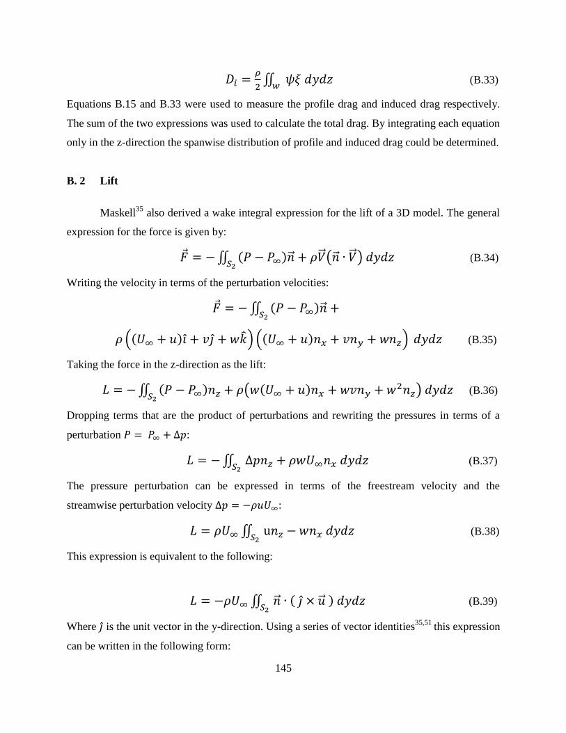
145

∬

(B.33)

Equations B.15 and B.33 were used to measure the profile drag and induced drag respectively.

The sum of the two expressions was used to calculate the total drag. By integrating each equation

only in the z-direction the spanwise distribution of profile and induced drag could be determined.

B. 2 Lift

Maskell35

also derived a wake integral expression for the lift of a 3D model. The general

expression for the force is given by:

∬ ( ) ( )

(B.34)

Writing the velocity in terms of the perturbation velocities:

∬ ( )

(( ) ) (( ) ) (B.35)

Taking the force in the z-direction as the lift:

∬ ( ) ( ( ) )

(B.36)

Dropping terms that are the product of perturbations and rewriting the pressures in terms of a

perturbation :

∬

(B.37)

The pressure perturbation can be expressed in terms of the freestream velocity and the

streamwise perturbation velocity :

∬

(B.38)

This expression is equivalent to the following:

∬ ( )

(B.39)

Where is the unit vector in the y-direction. Using a series of vector identities35,51

this expression

can be written in the following form:

146

∬

(B.40)

As was the case for the induced drag expression since the vorticity is zero outside of the wake

region the expression for lift can be expressed as a wake integral.

∬

(B.41)

The sectional lift coefficient can be determined from classical wing theory by assuming a planar

wake.33

The local vorticity strength of the vortex sheet is given by:

( ) ∫ ( )

(B.42)

The bound vortex strength is determined by integrating the vorticity along the vortex sheet.

( ) ∫ ( )

(B.43)

The Kutta-Joukowksi theorem can be used to relate the bound circulation to the sectional lift

coefficient.

( )

( ) ( ) (B.44)

Where c(y) is the local chord distribution.

B. 3 Summary of Wake Survey Integrals

Expressions for the profile drag, induced drag and the lift on a 3D model in terms of

quantities measured in the wake have been derived. These expressions are restated here.

∬ (( )

( )( ( )))

(B.45)

∬

(B.46)

∬

(B.47)

All expressions are in the form of wake integrals which allows for a significant reduction in the

amount of time necessary to acquire the measurements. Using these expressions the profile drag

and induced drag are determined separately from each other which provides an increased

understanding of the performance of the wing. In addition, these expressions provide spanwise

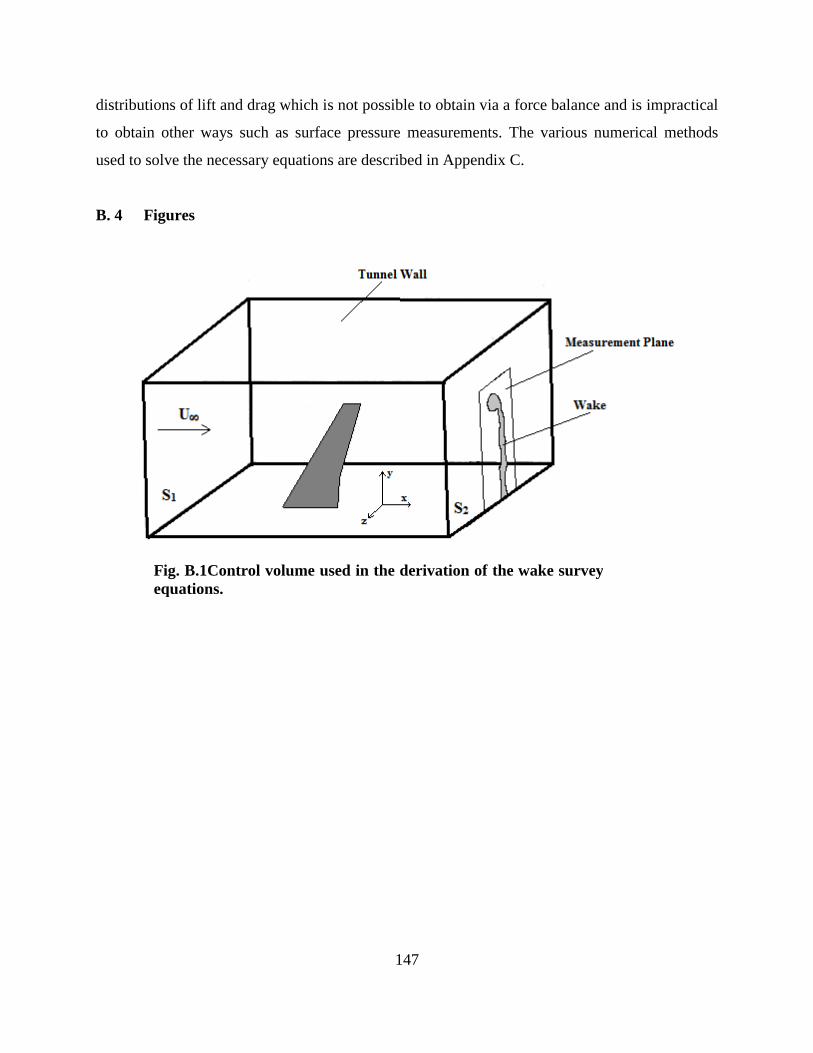
147

distributions of lift and drag which is not possible to obtain via a force balance and is impractical

to obtain other ways such as surface pressure measurements. The various numerical methods

used to solve the necessary equations are described in Appendix C.

B. 4 Figures

Fig. B.1Control volume used in the derivation of the wake survey

equations.

148

Appendix C

Wake Survey Data Reduction Methods

This appendix discusses the wake survey data reduction procedure to obtain lift and drag.

A description of the numerical methods used to solve the equations discussed in Appendix B will

be given. Throughout this appendix actual wake survey results will be used to illustrate the

various methods however these results will not be discussed in the context of aircraft icing. All

wake survey data reduction was done in Matlab.

C. 1 Preliminary Data Reduction

The first step in reducing the wake data was to apply the calibration discussed in

Appendix A. The calibration file for the desired Reynolds number was read into Matlab, the

pressure coefficients were calculated and interpolating surfaces were created using

TriScatteredInterp as discussed in Appedix A. The measurements from the wake survey were

then read into Matlab and the data were interpolated onto an evenly spaced mesh. The mesh

spacing was 0.25-inches which corresponded to the smallest probe spacing during data

acquisition. This was primarily done to simplify data storage in Matlab and to simplify the

numerical procedures. Interpolating all of the data onto a finer grid of 0.125-inches was

attempted to determine if the finer spacing improved results. Unfortunately this was not the case,

interpolating the data onto a finer grid decreased the accuracy of the results likely due to errors

introduced during the interpolation. Once the calibration was applied the values of , ,

and were known at each grid point. The flow angles were then transformed to the wing

coordinate system. Recall this was very straightforward; and . From the flow

angles and the total and static pressure coefficients the values of U, V and W were determined at

each grid point. The streamwise vorticity, defined in Eq. B.17, was calculated using a second

order central differencing method to differentiate the transverse velocity components (V and W).

On the edges of the measurement plane, second order forwards and backwards differencing were

used.

149

C. 2 Finding the Wake

The wake survey equations derived in Appendix B require integrations over the viscous

wake region. Ideally the various integrands in the equations for lift and drag would be zero

outside of the wake; however, due to experimental error this was not the case and it became

necessary to determine the edges of the wake. The wake was found using the following

procedure. First the total pressure loss coefficient at each grid point was calculated.

(C.1)

Next the derivative of the total pressure loss with respect to the non-dimensional Z coordinate (Z

= 2z/b) was calculated at each interior point using a second order central differencing method.

Then beginning at the negative Z boundary and the positive Z boundary, the wake was

approached along a line of constant Y = 2y/b, and at each point the absolute value of the

derivative was checked against a threshold. The threshold was set equal to 1.

(

)

(C.2)

Once the magnitude of the derivative surpassed this threshold it was assumed that the edge of the

wake had been found. The process was repeated for all Y locations. The vorticity and the total

pressure loss coefficient were set to zero at all points outside of the wake. By setting these values

to zero the integration could still be performed over the rectangular measurement plane

simplifying the data processing. The derivative of the total pressure loss coefficient was used

because this quantity varied smoothly with little noise. The total pressure coefficient could have

been used as well. The threshold value of 1 was chosen after visually inspecting several plots of

the derivative of the total pressure loss coefficient. Figures C.1 and C.2 show the normalized

streamwise vorticity throughout the entire measurement plane and only the wake respectively for

the clean wing at α = 4º and Re = 6x105. In Fig. C.1 streamwise vorticity on the order of a few

percent of the maximum is seen throughout the entire measurement plane. Including this

vorticity in the wake integrations can result in significant error. In Fig. C.2 this extraneous

vorticity has been removed leaving only the vorticity in the wake of the wing. The ability of this

method to isolate the wake is more clearly seen in Figs. C3 and C4 which show the total pressure

coefficient throughout the entire measurement plane and only the wake respectively for the clean

wing at α = 4º and Re = 6x105. Clearly the method described above effectively isolates the wake

without removing any of the measurements in the wake.

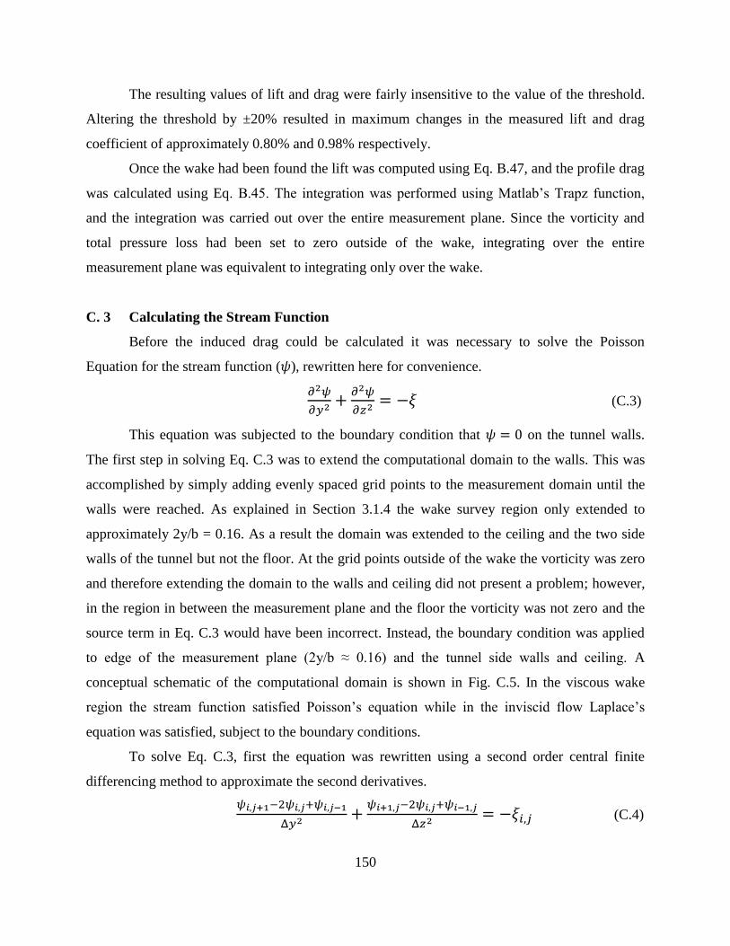
150

The resulting values of lift and drag were fairly insensitive to the value of the threshold.

Altering the threshold by ±20% resulted in maximum changes in the measured lift and drag

coefficient of approximately 0.80% and 0.98% respectively.

Once the wake had been found the lift was computed using Eq. B.47, and the profile drag

was calculated using Eq. B.45. The integration was performed using Matlab’s Trapz function,

and the integration was carried out over the entire measurement plane. Since the vorticity and

total pressure loss had been set to zero outside of the wake, integrating over the entire

measurement plane was equivalent to integrating only over the wake.

C. 3 Calculating the Stream Function

Before the induced drag could be calculated it was necessary to solve the Poisson

Equation for the stream function ( ), rewritten here for convenience.

(C.3)

This equation was subjected to the boundary condition that on the tunnel walls.

The first step in solving Eq. C.3 was to extend the computational domain to the walls. This was

accomplished by simply adding evenly spaced grid points to the measurement domain until the

walls were reached. As explained in Section 3.1.4 the wake survey region only extended to

approximately 2y/b = 0.16. As a result the domain was extended to the ceiling and the two side

walls of the tunnel but not the floor. At the grid points outside of the wake the vorticity was zero

and therefore extending the domain to the walls and ceiling did not present a problem; however,

in the region in between the measurement plane and the floor the vorticity was not zero and the

source term in Eq. C.3 would have been incorrect. Instead, the boundary condition was applied

to edge of the measurement plane (2y/b ≈ 0.16) and the tunnel side walls and ceiling. A

conceptual schematic of the computational domain is shown in Fig. C.5. In the viscous wake

region the stream function satisfied Poisson’s equation while in the inviscid flow Laplace’s

equation was satisfied, subject to the boundary conditions.

To solve Eq. C.3, first the equation was rewritten using a second order central finite

differencing method to approximate the second derivatives.

(C.4)

151

A constant stepsize was used in both directions, . By prescribing an initial guess

Eq. C.4 was solved using a Jacobi iteration method.

(

) (C.5)

The initial guess was over the entire domain. In order to satisfy the boundary conditions

the iterative process was only applied to the interior points forcing the value at the boundary to

remain zero. During each iteration was determined for each interior point. Then the

maximum difference between the current iteration and the previous iteration was checked against

an error tolerance threshold. If the difference was above the given threshold the interior points

were updated,

, and the process was repeated. Once the stream function was

determined the induced drag was calculated using Eq. B. 46. The effect of the error tolerance on

the calculated induced drag for the clean and iced wing at α = 4º and Re = 6x105

is shown in Fig.

C.6. Note that Fig. C.6 is a semi-log plot and that the induced drag is plotted against the inverse

of the error tolerance. This was done to clearly show the effect of decreasing the acceptable

error. As can be seen in Fig. C.6 the induced drag becomes insensitive to the value of the

tolerance for e greater than 10-5

. This value was consistent for all angles of attack of the clean

and iced wing. Since the increase in computational time was negligible e = 10-6

was used for the

final results. Once the induced drag was determined, the total drag was calculated by simply

adding the induced and profile drag.

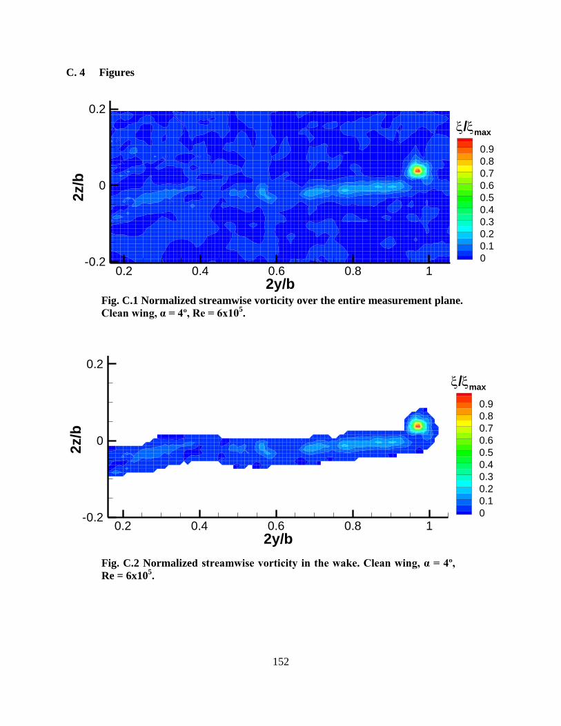
152

C. 4 Figures

Fig. C.1 Normalized streamwise vorticity over the entire measurement plane.

Clean wing, α = 4º, Re = 6x105.

2y/b

2z/b

0.2 0.4 0.6 0.8 1-0.2

0

0.2

0.4

0.9

0.8

0.7

0.6

0.5

0.4

0.3

0.2

0.1

0

/max

Fig. C.2 Normalized streamwise vorticity in the wake. Clean wing, α = 4º,

Re = 6x105.

2y/b

2z/b

0.2 0.4 0.6 0.8 1-0.2

0

0.2

0.4

0.9

0.8

0.7

0.6

0.5

0.4

0.3

0.2

0.1

0

/max

153

2y/b

2z/b

0.2 0.4 0.6 0.8 1-0.2

0

0.2

0.4

0.6

1

0.96

0.92

0.88

0.84

0.8

0.76

0.72

0.68

0.64

0.6

Cp,t

Fig. C.3 Total pressure coefficient over the entire measurement plane.

Clean wing, α = 4º, Re = 6x105.

2y/b

2z/b

0.2 0.4 0.6 0.8 1-0.2

0

0.2

0.4

1

0.96

0.92

0.88

0.84

0.8

0.76

0.72

0.68

0.64

0.6

Cp,t

Fig. C.4 Total pressure coefficient in the wake. Clean wing, α = 4º, Re = 6x105.

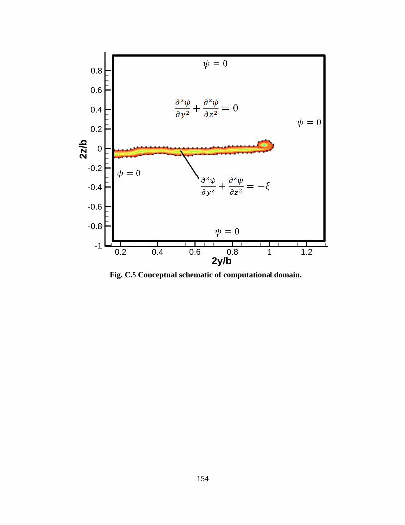
154

2y/b

2z/b

0.2 0.4 0.6 0.8 1 1.2-1

-0.8

-0.6

-0.4

-0.2

0

0.2

0.4

0.6

0.8

Fig. C.5 Conceptual schematic of computational domain.

155

1/e

CD

i

102

103

104

105

106

1070.0E+00

1.0E-03

2.0E-03

3.0E-03

4.0E-03

5.0E-03

6.0E-03

7.0E-03

8.0E-03 Clean

Ice

Fig. C.6 Effect of error tolerance in the calculation of ψ on the induced drag

of the clean and iced wing. α = 4º, Re = 6x105.

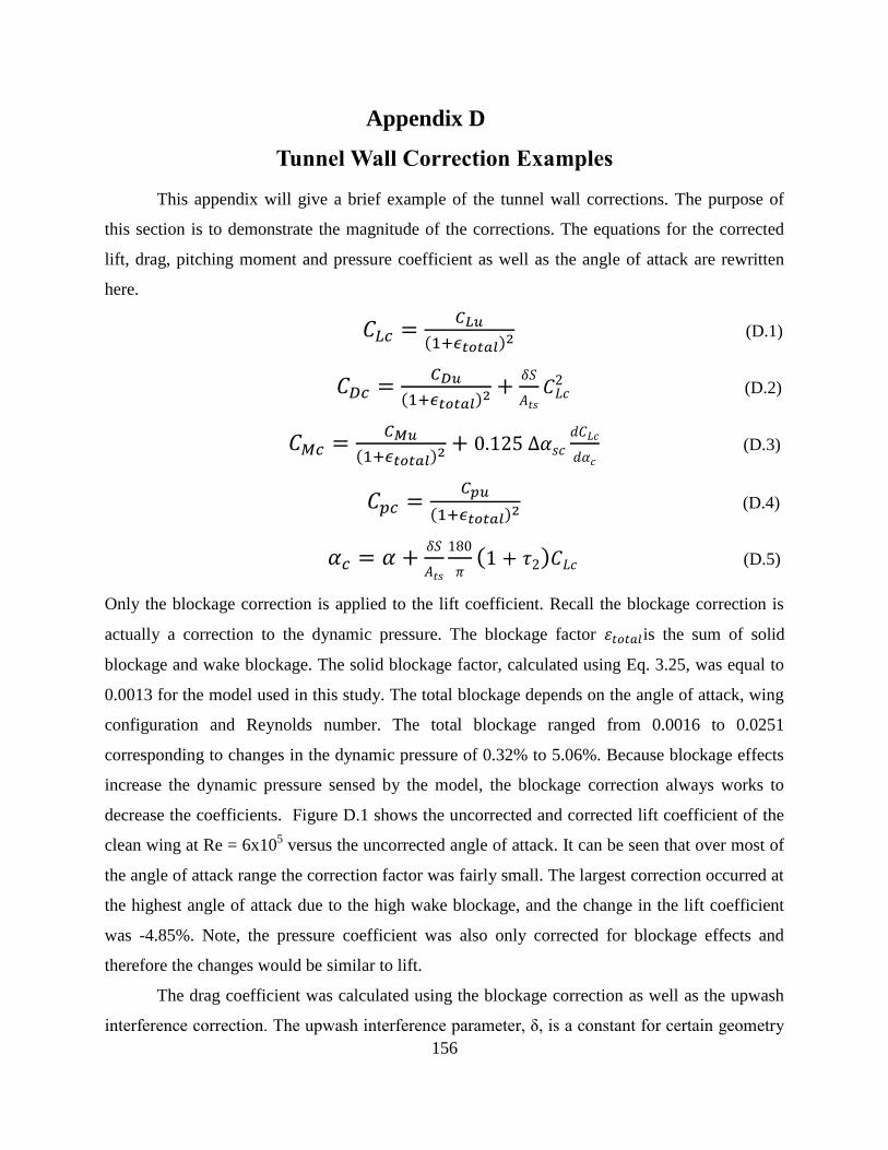
156

Appendix D

Tunnel Wall Correction Examples

This appendix will give a brief example of the tunnel wall corrections. The purpose of

this section is to demonstrate the magnitude of the corrections. The equations for the corrected

lift, drag, pitching moment and pressure coefficient as well as the angle of attack are rewritten

here.

( ) (D.1)

( )

(D.2)

( )

(D.3)

( ) (D.4)

( ) (D.5)

Only the blockage correction is applied to the lift coefficient. Recall the blockage correction is

actually a correction to the dynamic pressure. The blockage factor is the sum of solid

blockage and wake blockage. The solid blockage factor, calculated using Eq. 3.25, was equal to

0.0013 for the model used in this study. The total blockage depends on the angle of attack, wing

configuration and Reynolds number. The total blockage ranged from 0.0016 to 0.0251

corresponding to changes in the dynamic pressure of 0.32% to 5.06%. Because blockage effects

increase the dynamic pressure sensed by the model, the blockage correction always works to

decrease the coefficients. Figure D.1 shows the uncorrected and corrected lift coefficient of the

clean wing at Re = 6x105 versus the uncorrected angle of attack. It can be seen that over most of

the angle of attack range the correction factor was fairly small. The largest correction occurred at

the highest angle of attack due to the high wake blockage, and the change in the lift coefficient

was -4.85%. Note, the pressure coefficient was also only corrected for blockage effects and

therefore the changes would be similar to lift.

The drag coefficient was calculated using the blockage correction as well as the upwash

interference correction. The upwash interference parameter, δ, is a constant for certain geometry

157

and was equal to 0.14 in this study. Figure D.2 compares the uncorrected and corrected drag

coefficient of the clean wing at Re = 6x105 plotted against the uncorrected angle of attack. The

corrections had a larger effect on drag than on lift, the maximum change in drag due to the

correction was +16.8%. Equation D.2 shows that the blockage correction and interference

correction have opposite effect on the drag for positive values of the lift coefficient. At low

angles of attack these effects nearly cancelled out and the total correction was small. As the lift

increased the interference correction dominated and the corrected drag was substantially higher.

As the wing stalled the blockage correction began to increase while the interference correction

remained relatively constant due to the small changes in lift post stall. As a result the total

correction decreased and the two corrections nearly cancelled each other out at the highest

angles.

The pitching moment was corrected for blockage effects, upwash interference and

streamline curvature. Figure D.3 compares the uncorrected and corrected pitching moment

coefficient of the clean wing at Re = 6x105 plotted against the uncorrected angle of attack.

Similar to the lift coefficient, the wall corrections resulted in small changes to the pitching

moment. The largest change occurred at the highest angle of attack due to the high total

blockage. The maximum change due to the correction was 5.27%.

Finally, the angle of attack was corrected for upwash interference and streamline

curvature. Figure D.2 compares the uncorrected lift coefficient plotted against the uncorrected

angle of attack and the corrected angle of attack. The figure shows that the corrections increase

the angle of attack of the wing. The average increase was approximately 0.5º but reached a

maximum of 0.72º at the highest angle of attack.

158

uncor

CL

-10 -5 0 5 10 15 20-0.4

-0.2

0

0.2

0.4

0.6

0.8

1

Uncorrected Lift

Corrected Lift

Fig. D.1 Comparison of uncorrected and corrected lift coefficient

plotted against the uncorrected angle of attack. Clean wing, Re = 6x105

uncorr

CD

-10 -5 0 5 10 15 200

0.05

0.1

0.15

0.2

0.25

Uncorrected Drag

Corrected Drag

Fig. D.2 Comparison of uncorrected and corrected drag coefficient for the clean wing

plotted against the uncorrected angle of attack. Clean wing, Re = 6x105

159

uncorr

CM

-10 -5 0 5 10 15 20-0.3

-0.25

-0.2

-0.15

-0.1

-0.05

0

0.05

0.1

Uncorrected Moment

Corrected Moment

Fig. D.3 Comparison of uncorrected and corrected pitching moment coefficient for the

clean wing plotted against the uncorrected angle of attack. Clean wing, Re = 6x105

CL

,un

co

rr

-10 -5 0 5 10 15 20-0.4

-0.2

0

0.2

0.4

0.6

0.8

1

Uncorrected

Corrected

Fig. D.4 Comparison of uncorrected lift coefficient plotted against the

uncorrected and the corrected angle of attack. Clean wing, Re = 6x105

160

Appendix E

Uncertainty Analysis

This appendix will provide the results of uncertainty analysis of the force balance

measurements. The uncertainties were calculated using the method of Kline and McClintock.52

Throughout this appendix the variable represents the uncertainty in the measured quantity r.

The relative uncertainties of the lift, drag and pitching moment coefficients are given by the

following expressions. A detailed derivation of these expressions can be found in Ansell.53

√(

) (

) (

)

(E.1)

√(

) (

) (

)

(E.2)

√(

)

(

) (

) (

)

(E.3)

Where , and represent the uncertainties in the measured lift, drag and

pitching moment in dimensional units. They are functions of the uncertainties in the measured

normal force ( ), axial force (

) and pitching moment about the quarter chord ( ) as

well as the uncertainty in the angle of attack ( ).

161

√( )

(

) ( ) (E.4)

√( )

(

) ( ) (E.5)

√( ) (

) (

) (

) (

) (E.6)

In Eq. E6, represents the uncertainty in the moment measured about the center of the

balance while and respresent the offset of the quarter chord from the center of the

balance as discussed in Section 3.1.3.1. It was assumed that the uncertainty in both offsets was

0.02 inches. The relative uncertainties in the normal force, axial force and moment about balance

center were 0.02%, 0.03% and 0.15%, respectively, of full-scale. Since the balance was set to the

low Load Range, as discussed in Section 3.1.3.1, the absolute uncertainties in normal force, axial

force and moment were 0.018 lbs, 0.0054 lbs, and 0.0225 ft-lbs. The uncertainty in the angle of

attack ( ) was 0.02º. The dynamic pressure was measured directly using a ±1.0 psid module,

therefore the uncertainty in dynamic pressure ( ) corresponded to the uncertainty in the

module which was ±0.001 psi. The uncertainty in the planform area ( ) was due to the

tolerances of the SLA process which were given by the manufacture as 0.001-in. per inch. The

span of the model was 25.1-in. and the mean aerodynamic chord was 6.98-in. The corresponding

uncertainties in the span and mean aerodynamic chord ( ) were 0.0251-in. and 0.0069-in,

respectively. Assuming the uncertainty in the planform area is approximately proportional to the

product of the uncertainty in the span and the mean aerodynamic chord, then = 1.75x10-4

-in2.

These uncertainties are all summarized in Table E.1. Note that the reference values for the loads,

angle of attack and dynamic pressure corresponded to the clean wing at a lift coefficient of 0.5

for Re = 6x105.

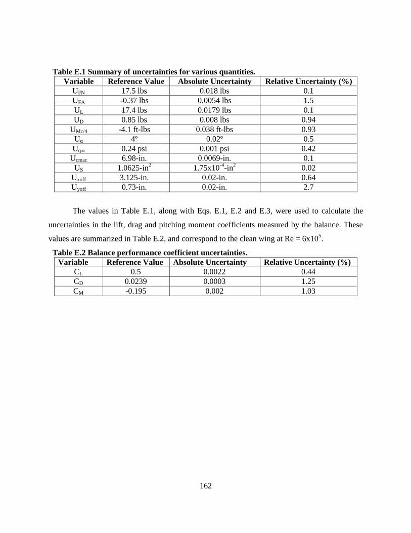
162

Table E.1 Summary of uncertainties for various quantities.

Variable Reference Value Absolute Uncertainty Relative Uncertainty (%)

UFN 17.5 lbs 0.018 lbs 0.1

UFA -0.37 lbs 0.0054 lbs 1.5

UL 17.4 lbs 0.0179 lbs 0.1

UD 0.85 lbs 0.008 lbs 0.94

UMc/4 -4.1 ft-lbs 0.038 ft-lbs 0.93

Uα 4º 0.02º 0.5

Uq∞ 0.24 psi 0.001 psi 0.42

Ucmac 6.98-in. 0.0069-in. 0.1

US 1.0625-in2 1.75x10

-4-in

2 0.02

Uxoff 3.125-in. 0.02-in. 0.64

Uyoff 0.73-in. 0.02-in. 2.7

The values in Table E.1, along with Eqs. E.1, E.2 and E.3, were used to calculate the

uncertainties in the lift, drag and pitching moment coefficients measured by the balance. These

values are summarized in Table E.2, and correspond to the clean wing at Re = 6x105.

Table E.2 Balance performance coefficient uncertainties.

Variable Reference Value Absolute Uncertainty Relative Uncertainty (%)

CL 0.5 0.0022 0.44

CD 0.0239 0.0003 1.25

CM -0.195 0.002 1.03

163

References

1 Lynch, F.T. and Khodadoust, A., “Effects of Ice Accretions on Aircraft Aerodynamics,”

Progress in Aerospace Sciences, Vol. 37, p. 669-767, 2001. 2Bragg, M.B.; Broeren, A.P.; and Blumenthal, L.A., “Iced-Airfoil Aerodynamics,” Prog. Aerosp.

Sci., vol. 41, no. 5, 2005, pp. 323–362. 3 Furlong, G.C., and McHugh, J.G., “A Summary and Analysis of the Low-Speed Longitudinal

Characteristics of Swept Wings at High Reynolds Number,” NACA TR-1339, 1952. 4 Hoerner, S.F., Fluid-Dynamic Lift, Hoerner Fluid Dynamics, Brick Town, NJ, 1975.

5 Papadakis, M., Yeong, H.W. and Wong, S.C, “Aerodynamic Performance of a Swept Wing

with Ice Accretions,” AIAA 2003-0731 6 Papadakis, M., Yeong, H.W. and Wong, S.C, “Aerodynamic Performance of a Swept Wing

with Simulated Ice Shapes,” AIAA 2004-0734 7 Khodadoust, A. and Bragg, M.B., “Aerodynamics of a Finite Swept Wing with Simulated Ice,”

Journal of Aircraft, Vol. 32, No. 1, pp 137-144, 1995. 8 Bragg, M.B., Kerho, M.F., Khodadoust, A., “LDV Flowfield Measurements on a Straight and

Swept Wing with a Simulated Ice Accretion,” AIAA 1993-0300. 9 Broeren, A.P. "Swept-Wing Ice Accretion Characterization and Aerodynamics--Research Plans

and Current Status," NASA Aviation Safety Program Annual Technical Meeting, St. Louis, MO,

May 10-12, 2011. 10

Katz, J. and Plotkin, A., Low Speed Aerodynamics. Cambridge University Press, New York,

2001. 11

Kuchemann, D., “Types of Flow on Swept Wings,” Royal Aircraft Establishment 12

McCullough, G.B. and Gault, D.E., “Examples of Three Representative Types of Airfoil

Section Stall at Low Speed,” NACA TN 2502. 13

Harper, C.W., and Maki, R.L., “A Review of the Stall Characteristics of Swept Wings,”

NASA TN D-2373 14

Anderson, R. F., “Determination of the Characteristics of Tapered Wings,” NACA Rep. 572,

1936. 15

Hunton, L.W. and James, H.A., “Use of Two-Dimensional Data in Estimating Loads on a 45˚

Sweptback Wing with Slats and Partial-Span Flaps,” NACA TN 3040, 1953. 16

Polhamus, E.C., “A Survey of Reynolds Number and Wing Geometry Effects on Lift

Characteristics in the Low Speed Stall Region,” NASA CR 4747, 1996. 17

Boltz, F.W. and Kolbe, C.D, “The Forces and Pressure Distribution at Subsonic Speeds on a

Cambered and Twisted Wing Having 45˚ Sweepback, Aspect Ratio of 3 and Taper Ratio of 0.5,”

NACA RM A52D22 1952. 18

Poll, D.I.A., “Spiral Vortex Flow Over a Swept-Back Wing,” Aeronautical Journal, May 1986. 19

Mirande, J., Schmitt, V. and Werle, H., “Vortex Pattern Developing on the Upper Surface of a

Swept Wing at High Angle of Attack,” Office Natinal d’Etudes et de Recherches Aerospatiales

(ONERA). 20

Haines, A.B., “Scale effects on Weapon and Aircraft Aerodynamics,” AGARD AG-323, Jul

1994.

164

21 Polhamus, E.C., “A Concept of the Vortex Lift of Sharp Edge Delta Wings Based on Leading-

Edge Suction Analogy,” AIAA 1959-1133, 1969. 22

Tinling, B.E. and Lopez, A.E., “The Effects of Reynolds Number at Mach Numbers up to 0.94

on the Loading on a 35˚ Swept Back Wing Having NACA 651A012 Streamwise Sections,”

NACA RM A52B20. 23

Kim H.S, Bragg M.B., “Effects of Leading-Edge Ice Accretion Geometry on Airfoil

Aerodynamics,” AIAA Paper 99-3150, 1999. 24

Roberts, W.B., “Calculation of Laminar Separation Bubbles and Their Effect on Airfoil

Performance,” AIAA J., 1980, Vol. 18, pg. 25-31. 25

Bragg, M.B., Khodadoust, A and Spring, A.S., “Measurements in a Leading-Edge Separation

Bubble Due to a Simulated Airfoil Ice Accretion,” AIAA J., Vol 30, no. 6, pg. 1462-1470, 1992. 26

Vargas, M., “Current Experimental Basis for Modeling Ice Accretions on Swept Wings,”

Journal of Aircraft, Vol. 44, No. 1, Jan.-Feb. 2007, pp. 274-290. 27

Vargas, M. and Reshotko, E., “Parametric Experimental Study of the Formation of Glaze Ice

Shapes on Swept Wings,” AIAA 1999-0094. 28

Vargas, M., Papadakis, M., Potapczuk, M.G., Addy, H.E. Jr., Sheldon, D. and Giriunas, J.,

“Ice Accretions on a Swept GLC-305 Airfoil.” SAE 02GAA-43, SAE General Aviation

Technology Conference and Exhibition, Wichita, KS, Apr. 2002, Also NASA/TM—2002-

211557, Apr. 2002. 29

Papadakis, M., Alansatan, S., and Yeong, H.W., “Aerodynamic Performance of a T-Tail with

Simulated Ice Accretions,” 38th

Aerospace Sciences Meeting & Exhibit, AIAA 2000-0363 30

Kwon, O.J. and Sankar, L.N., “Numerical Study of the Effects of Icing on Fixed and Rotary

Wing Performance,” AIAA 1991-0662 31

Vassberg, J.C., DeHaan, M.A., Rvers, S.M. and Wahls, R.A., “Development of a Common

Research Model for Applied CFD Validation Studies,” AIAA 2008-6929 32

Brune, G., W., “Quantitative Low Speed Wake Surveys,” Journal of Aircraft Vol. 31, No. 2,

1994. 33

Kusunose, K,. “Development of a Universal Wake Survey Data Analysis Code,” AIAA 199-

2294. 34

Betz, A., “A Method for the Direct Determination of Profile Drag,” ZFM, Vol. 16, pp.42, 1925 35

Maskell, E.C., “Progress Towards a Method for the Measurement of the Components of the

Drag of a Wing of Finite Span,” RAE Technical Report 72232, 1972. 36

Pope, A., Rae, W.H., and Barlow, J.B., “Low-Speed Wind Tunnel Testing,” John Wley &

Sons, Inc., 3rd

ed., 1999. 37

Thom, A., “Blockage Correction in a High Speed Wind Tunnel,” ARC R&M 2033, 1943. 38

Makell, E.C., “A Theory of the Blockage Effects on Bluff Bodies and Stalled Wings in a

Closed Tunnel,” ARC R&M 3400, 1965. 39

Garner, H.C., Rogers, E.W.E, Acum, W.E.A. and Maskell, E.C., “Subsonic Wind Tunnel

Corrections,” AGARDograph 109, 1966. 40

Polhamus, E.C., “Jet Boundary Induced Upwash Velocities for Swept Reflection Plane Models

Mounted Vertically in a 7 by 10 Foot Closed Rectangular Tunnel,” NACA TN 1752. 41

Potapczuk, M.G., Papadakis, M.J., and Vargas, M., “LEWICE Modeling of Swept Wing Ice

Accretions,” AIAA 2003-0730

165

42 Meschia, F., “Model Analysis with XFLRT,” Radio Controlled Soaring Digest, Vol. 25, No.

2, February 2008, pp. 27-51. 43

Drela, M., “XFOIL 6.96 User Primer,” MIT Aero & Astro Engineering, May 3, 2006. 44

Winkler, J.F., “Local Flowfield about Large Distributed Roughness Elements in a Laminar

Boundary Layer”, Ph.D. Thesis, University of Illinois at Urbana-Champaign, Urbana, IL, 1996. 45

Diebold, J.M, Monastero, M.C. and Bragg, M.B., “Aerodynamics of a Swept Wing with Ice

Accretion at Low Reynolds Number,” 30th

AIAA Applied Aerodynamics Conference, AIAA

2012-2795. 46

Broeren, A.P., Lee, S., Shah, G.H. and Murphy, P.C., “Aerodynamic Effects of Simulated Ice

Accretion on a Generic Transport Model,” SAE Technical Paper 2011-38-0065 47

Witkowski, D., Lee, A. and Sullivan, J., “Aerodynamic Interaction Between Propellers and

Wings,” Journal of Aircraft, Vol. 26, No. 9, p. 829-836, 1989. 48

Treaster, A.L. and Yocum, A.M., “The Calibration and Application of Five-Hole Probes,”

NAVSEA, Technical Memorandum 78-10, 1978. 49

Hackett, J.E. and Sugavanam, A., “Evaluation of a Complete Wake Integral for the Drag of a

Car-Like Shape,” SAE Technical Paper 840577, 1984. 50

Wu, J.C., Hackett, J.E. and Liley, D.E., “A Generalized Wake-Integral Approach for Drag

Determination in Three-Dimensional Flows,” AIAA 1979-0279 51

Cummings, R.M., Giles, M.B. and Shrinivas, G.N., “Analysis of the Elements of Drag in a

Three-Dimensional Viscous and Inviscid Flow,” AIAA 1996-2482 52

Kline, S. and McClintock, F. A., “Describing Uncertainty in Single-Sample Experiments,”

Mechanical Engineering, Vol. 75, 1953, pp. 3–8. 53

Ansell, P.J., “Flight Envelope Protection Using Flap Hinge Moment Measurement”, M.S.

Thesis, University of Illinois at Urbana-Champaign, Urbana, IL, 2010.