> >

> >

(8)(8)

Exercise 3: Find all solutions to the linear (and also separable) DE

y x =6 x 3 x y

x2 1

Hint: as you can verify below, the general solution is y x = 2 C x2 1

32

.with DEtools :

dsolve y x =6 x 3 x y x

x2 1, y x ; #Maple check

y x = 2_C1

x2 13 / 2

> >

An extremely important class of modeling problems that lead to linear DE's involve input-output models. These have diverse applications ranging from bioengineering to environmental science. For example, The "tank" below could actually be a human body, a lake, or a pollution basin, in different applications.

For the present considerations, consider a tank holding liquid, with volume V t (e.g units l ). Liquid

flows in at a rate ri (e.g. units ls

), and with solute concentration ci (e.g. units gml

). Liquid flows out at a

rate ro , and with concentration c0 . We are attempting to model the volume V t of liquid and the amount of solute x t (e.g. units gm ) in the tank at time t , given V 0 = V0, x 0 = x0 . We assume the solution in the tank is well-mixed, so that we can treat the concentration as uniform throughout the tank, i.e.

co =x tV t

gml

.

See the diagram below.

Exercise 4: Under these assumptions use your modeling ability and Calculus to derive the following differential equations for V t and x t :a) The DE for V t , which we can just integrate:

V t = ri r0

so V t = V00

tri r0 d

b) The linear DE for x t .

x t = ri ci ro co = ri ci roxV

x troVx t = ri ci

> >

Often (but not always) the tank volume remains constant, i.e. ri = ro . If the incoming concentration ci is also constant, then the IVP for solute amount is

x a x = b x 0 = x0

where a, b are constants. This differential equation is separable and linear, and it is recommended that you become good at solving it. Notice that it includes the exponential growth/decay and Newton's law of cooling DE's as special cases.

> >

> >

(1)(1)

Math 2250-004 Week 3 notes, Jan 23-27

Mon Jan 231.5: linear DEs, and applications.

Recall from Friday notes (review/cover if necessary) that input-out models often lead to the IVPx a x = b

x 0 = x0 where a, b are (positive) constants.

Exercise 1: The constant coefficient initial value problem above will recur throughout the course in various contexts, so let's solve it now. We might check our answer with Wolfram alpha. Maple check is below.

x t =ba

xoba

e a t .

with DEtools : dsolve x t a x t = b, x 0 = x0 ;

x t =ba

e a t x0ba

Exercise 2: Use the result above to solve a pollution problem IVP and answer the following question (p. 55-56 text): Lake Huron has a pretty constant concentration for a certain pollutant. Due to an industrial accident, Lake Erie has suddenly obtained a concentration five times as large. Lake Erie has a volume of 480 km3 , and water flows into and out of Lake Erie at a rate of 350 km3 per year. Essentially all of the in-flow is from Lake Huron (see below). We expect that as time goes by, the water from Lake Huron will flush out Lake Erie. Assuming that the pollutant concentration is roughly the same everywhere in Lake Erie, about how long will it be until this concentration is only twice the background concentration from Lake Huron?

http://www.enchantedlearning.com/usa/statesbw/greatlakesbw.GIFa) Set up the initial value problem. Maybe use symbolsc for the background concentration (in Huron), V = 480 km3

r = 350 km3

y

b) Solve the IVP, and then answer the question.

EP 3.7 This is a supplementary section. I've posted a .pdf on our homework page.

Often the same DE can arise in completely different-looking situations. For example, first order linear DE's also arise (as special cases of second order linear DE's) in simple RLC circuit modeling.

http://cnx.org/content/m21475/latest/pic012.png

Charge Q t coulombs accumulates on the capacitor, at a rate I t i t in the diagram above) amperes (coulombs/sec), i.e Q t = I t .Kirchoff's Law: The sum of the voltage drops around any closed circuit loop equals the applied voltage V t (volts). The units of voltage are energy units - Kirchoff's Law says that a test particle traversing any closed loop returns with the same potential energy level it started with:

For Q t : L Q t R Q t1C

Q t = V t

For I t : L I t R I t1C

I t = V t

if no inductor, or if no capacitor, then Kirchoff's Law yields 1st order linear DE's, as below:

Exercise 3: Consider the R L circuit below, in which a switch is thrown at time t = 0. Assume the voltage V is constant, and I 0 = 0 . Find I t . Interpret your results.

http://www.intmath.com/differential-equations/5-rl-circuits.php

Tues Jan 242.1 Improved population models

Let P t be a population at time t . Let's call them "people", although they could be other biological organisms, decaying radioactive elements, accumulating dollars, or even molecules of solute dissolved in a liquid at time t (2.1.23). Consider:

B t , birth rate (e.g. peopleyear

) ;

tB tP t

, fertility rate (peopleyear

per person )

D t , death rate (e.g. peopleyear

);

tD tP t

, mortality rate (peopleyear

per person )

Then in a closed system (i.e. no migration in or out) we can write the governing DE two equivalent ways:P t = B t D t

P t = t t P t .

Model 1: constant fertility and mortality rates, t 0 0, t 0 0 , constants.

P = 0 0 P = k P .This is our familiar exponential growth/decay model, depending on whether k 0 or k 0 .

Model 2: population fertility and mortality rates only depend on population P, but they are not constant:= 0 1P

= 0 1P

with 0, 1, 0, 1 constants. This implies

P = P = 0 1P 0 1P P

= 0 0 1 1 P P .

For viable populations, 0 0. For a sophisticated (e.g. human) population we might also expect

1 0, and resource limitations might imply 1 0. With these assumptions, and writing 1 1 = a

0, 0 0 = b 0 one obtains the logistic differential equation:P = b a P P P = b P a P2 , or equivalently

P = a Pba

P = k P M P .

k = a 0, M =ba

0 . (One can consider other cases as well.)

Exercise 1: Discuss qualitative features of the slope field for the logistic differential equation for P = P t :

P = k P M P

a) There are two constant ("equilibrium") solutions. What are they?

b) Evaluate the sign and magnitude of the slope function f P, t = k P M P , in order to understand and be able to recreate the two diagrams below. One is a qualititative picture of the slope field, in the t P plane. The diagram to the left of it, called the phase diagram , is just a P number line with arrows indicating whether P t is increasing or decreasing on the intervals between the constant solutions.

c) When discussing the logistic equation, the value M is called the "carrying capacity" of the (ecological orother) system. Discuss why this is a good way to describe M . Hint: if P 0 = P0 0 , and P t solves the logistic equation, what is the apparent value of lim

tP t ?

> >

Exercise 2: Solve the logistic DE IVPP = k P M P

P 0 = P0 via separation of variables. Verify that the solution formula is consistent with the slope field and phase diagram discussion from exercise 1. Hint: You should find that

P t =MP0

M P0 e Mkt P0

.

Solution (we will work this out step by step in class):dP

P P M= k dt

By partial fractions,1

P P M=

1M

1P M

1P

.

Use this expansion and multiply both sides of the separated DE by M to obtain1

P M1P

dP = kM dt .

Integrate:ln P M ln P = Mkt C1

lnP M

P= Mkt C1

exponentiate:P M

P= C2 e Mkt

Since the left-side is continuous

P M

P= C e Mkt (C = C2 or C = C2)

(At t = 0 we see thatP0 M

P0= C .)

Now, solve for P t by multiplying both sides of of the second to last equation by P t :P M = Ce MktP

Collect P t terms on left, and add M to both sides:P Ce MktP = M

P 1 Ce Mkt = M

P =M

1 Ce Mkt .

Plug in C and simplify:

P =M

1P0 M

P0e Mkt

=MP0

P0 P0 M e Mkt

P t =MP0

P0 M P0 e Mkt .

Finally, because limt

e Mkt = 0 , we see that

limt

P t =MP0

P0= M as expected.

Note: If P0 0 the denominator stays positive for t 0, so we know that the formula for P t is a differentiable function for all t 0. (If the denominator became zero, the function would blow up at the corresponding vertical asymptote.) To check that the denominator stays positive check that (i) if P0 M then the denominator is a sum of two positive terms; if P0 = M the separation algorithm actually fails because you divided by 0 to get started but the formula actually recovers the constant equilibrium solution P t M; and if P0 M then M P0 P0 so the second term in the denominator can never be negative enough to cancel out the positive P0 , for t 0 .)

Question: You have a couple of homework problems where you are asked to find solutions x t to differential equations of the form

x t = a x b x c .How would you proceed?

(2)(2)

> > (3)(3)

> >

> >

> >

> >

> >

> >

Application! The Belgian demographer P.F. Verhulst introduced the logistic model around 1840, as a tool for studying human population growth. Our text demonstrates its superiority to the simple exponential growth model, and also illustrates why mathematical modelers must always exercise care, by comparing the two models toactual U.S. population data.

restart : # clear memory Digits 5 : #work with 5 significant digitspops 1800, 5.3 , 1810, 7.2 , 1820, 9.6 , 1830, 12.9 , 1840, 17.1 , 1850, 23.2 , 1860, 31.4 , 1870, 38.6 , 1880, 50.2 , 1890, 63.0 , 1900, 76.2 , 1910, 92.2 , 1920, 106.0 , 1930, 123.2 , 1940, 132.2 , 1950, 151.3 , 1960, 179.3 , 1970, 203.3 , 1980, 225.6 , 1990, 248.7 , 2000, 281.4 , 2010, 308. : #I added 2010 - between 306-313 # I used shift-enter to enter more than one line of information # before executing the command.with plots : # plotting library of commands pointplot pops, title = `U.S. population through time` ;

1800 1850 1900 1950 2000

100

300U.S. population through time

Unlike Verhulst, the book uses data from 1800, 1850 and 1900 to get constants in our two models. We let t=0 correspond to 1800.

Exponential Model: For the exponential growth model P t = P0 er t we use the 1800 and 1900 data to get values for P0 and r :

P0 5.308;solve P0 exp r 100 = 76.212, r ;

P0 5.3080.026643

P1 t 5.308 exp .02664 t ;#exponential model -eqtn (9) page 83P1 t 5.308 e0.02664 t

> >

> >

> >

(6)(6)

> >

> >

(5)(5)

(4)(4)

> >

Logistic Model: We get P0 from 1800, and use the 1850 and 1900 data to find k and M :

P2 t M P0 / P0 M P0 exp M k t ; # logistic solution we worked out

P2 tM P0

P0 M P0 e M k t

solve P2 50 = 23.192, P2 100 = 76.212 , M, k ;M = 188.12, k = 0.00016772

M 188.12; k .16772e-3;P2 t ; #should be our logistic model function, #equation (11) page 84.

M 188.12k 0.00016772

998.545.308 182.81 e 0.031551 t

Now compare the two models with the real data, and discuss. The exponential model takes no account of the fact that the U.S. has only finite resources. Any ideas on why the logistic model begins to fail (with our parameters) around 1950?

plot1 plot P1 t 1800 , t = 1800 ..1950, color = black, linestyle = 3 : #this linestyle gives dashes for the exponential curveplot2 plot P2 t 1800 , t = 1800 ..2010, color = black :plot3 pointplot pops, symbol = cross :display plot1, plot2, plot3 , title = `U.S. population dataand models` ;

t1800 1850 1900 1950 2000

100

200

300

U.S. population dataand models

Math 2250-004Wednesday Jan 25

2.2: Autonomous Differential Equations.Recall, that if we solve for the derivative, a general first order DE for x = x t is written as

x = f t, x ,which is shorthand for x t = f t, x t . Definition: If the slope function f only depends on the value of x t , and not on t itself, then we call the first order differential equation autonomous:

x = f x .

Example: The logistic DE, P = k P M P is an autonomous differential equation for P t , for example.

Definition: Constant solutions x t c to autonomous differential equations x = f x are calledequilibrium solutions. Since the derivative of a constant function x t c is zero, the values c of equilibrium solutions are exactly the roots c to f c = 0 .

Example: The functions P t 0 and P t M are the equilibrium solutions for the logistic DE.

Exercise 1: Find the equilibrium solutions of 1a) x t = 3 x x2

1b) x t = x3 2 x2 x

1c) x t = sin x .

Def: Let x t c be an equilibrium solution for an autonomous DE. Then · c is a stable equilibrium solution if solutions with initial values close enough to c stay close to c. There is a precise way to say this, but it requires quantifiers: For every 0 there exists a 0 so that for solutions with x 0 c , we have x t c for all t 0 . · c is an unstable equilibrium if it is not stable. · c is an asymptotically stable equilibrium solution if it's stable and in addition, if x 0 is close enough to c , then lim

tx t = c, i.e. there exists a 0 so that if x 0 c then

limt

x t = c . (Notice that this means the horizontal line x = c will be an asymptote to the solution graphs x = x t in these cases.)

Exercise 2: Use phase diagram analysis to guess the stability of the equilibrium solutions in Exercise 1. For (a) you've worked out a solution formula already, so you'll know you're right. For (b), (c), use the Theorem on the next page to justify your answers.

2a) x t = 3 x x2

2b) x t = x3 2 x2 x

2c) x t = sin x .

Theorem: Consider the autonomous differential equationx t = f x

with f x and x

f x continuous (so local existence and uniqueness theorems hold). Let f c = 0 , i.e.

x t c is an equilibrium solution. Suppose c is an isolated zero of f, i.e. there is an open interval containing c so that c is the only zero of f in that interval. The the stability of the equilibrium solution c canis completely determined by the local phase diagrams:

sign f : 0 c c is unstable sign f : 0 c c is asymptotically stable

sign f : 0 c c is unstable (half stable) sign f : 0 c c is unstable (half stable)

You can actually prove this Theorem with calculus!! (want to try?)

Here's why!

Exercise 3) Use the chain rule to check that if x t solves the autonomous DEx t = f x

Then X t x t c solves the same DE. What does this say about the geometry of representative solution graphs to autonomous DEs? Have we already noticed this?

Further application: Doomsday-extinction. With different hypotheses about fertility and mortality rates, one can arrive at a population model which looks like logistic, except the right hand side is the opposite of what it was in that case:

Logistic: P t = a P2 b P Doomsday-extinction: Q t = a Q2 b Q

For example, suppose that the chances of procreation are proportional to population density (think alligators), i.e. the fertility rate = a Q t , where Q t is the population at time t. Suppose the morbidity rate is constant, = b. With these assumptions the birth and death rates are a Q2 and b Q .... which yields the DE above. In this case factor the right side:

Q t = a Q Qba

= k Q Q M .

Exercise 4a) Construct the phase diagram for the general doomsday-extinction model and discuss the stability of the equilbrium solutions.

Exercise 4b) If P t solves the logistic differential equationP t = k P M P

show that Q t P t solves the doomsday-extinction differential equationQ t = k Q Q M .

Use this to recover a formula for solutions to doomsday-extinction IVPs. What does this say about how representative solution graphs are related, for the logistic and the doomsday-extinction models? Recall, thesolution to the logistic IVP is

P t =MP0

M P0 e Mkt P0

.

Exercise 5) Use your formula from the previous exercise to transcribe the solution to the doomsday-extinction IVP

x t = x x 1x 0 = 2 .

Does the solution exist for all t 0 ? (Hint: no, there is a very bad doomsday at t = ln 2.

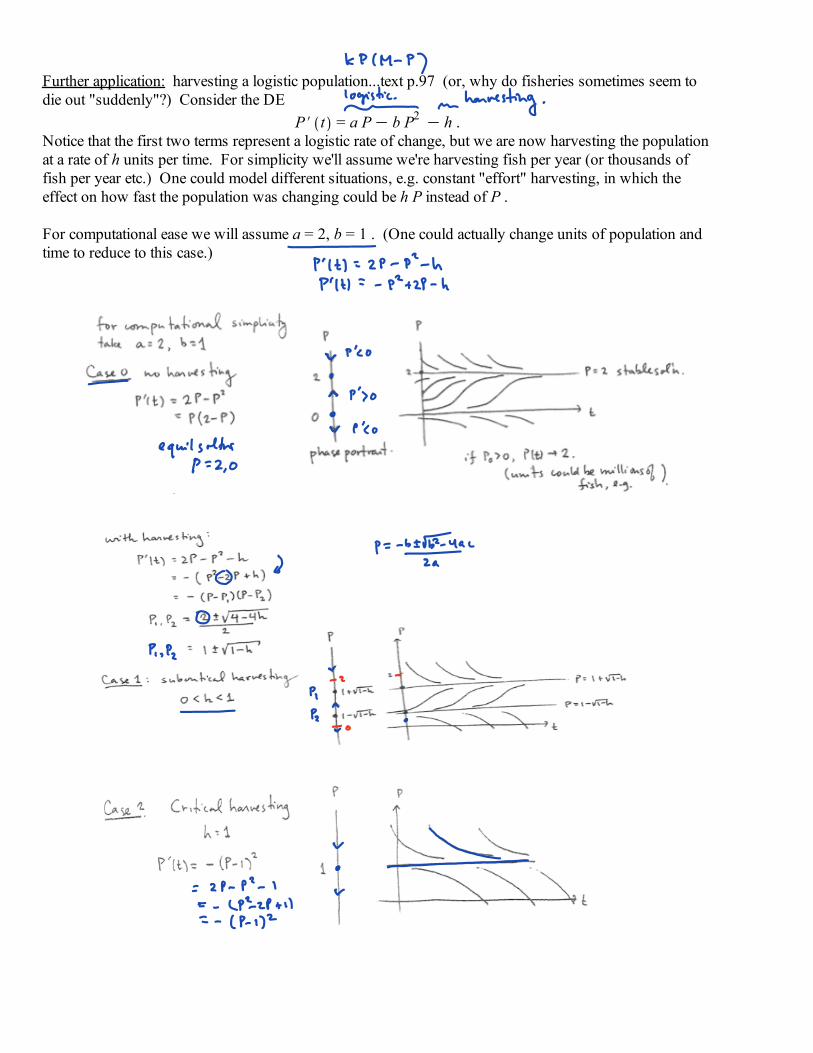
Further application: harvesting a logistic population...text p.97 (or, why do fisheries sometimes seem to die out "suddenly"?) Consider the DE

P t = a P b P2 h .Notice that the first two terms represent a logistic rate of change, but we are now harvesting the population at a rate of h units per time. For simplicity we'll assume we're harvesting fish per year (or thousands of fish per year etc.) One could model different situations, e.g. constant "effort" harvesting, in which the effect on how fast the population was changing could be h P instead of P .

For computational ease we will assume a = 2, b = 1 . (One could actually change units of population and time to reduce to this case.)

This model gives a plausible explanation for why many fisheries have "unexpectedly" collapsed in modernhistory. If h 1 but near 1 and something perturbs the system a little bit (a bad winter, or a slight increase in fishing pressure), then the population and/or model could suddenly shift so that P t 0 very quickly.

Here's one picture that summarizes all the cases - you can think of it as collection of the phase diagrams fordifferent fishing pressures h . The upper half of the parabola represents the stable equilibria, and the lowerhalf represents the unstable equilibria. Diagrams like this are called "bifurcation diagrams". In the sketch below, the point on the h- axis should be labeled h = 1 , not h . What's shown is the parabola of equilibrium solutions, c = 1 1 h , i.e. 2 c c2 h = 0 , i.e. h = c 2 c .

Math 2250-004 Fri Jan 27

2.3 Improved velocity models: velocity-dependent drag forces

For particle motion along a line, with position x t (or y t ,

velocity x t = v t , and acceleration x t = v t = a t

We have Newton's 2nd lawm v t = F

where F is the net force. We're very familiar with constant force F = m , where is a constant:

v t = v t = t v0

x t =12

t2 v0 t x0 .

Examples we've seen a lot of: = g near the surface of the earth, if up is the positive direction, or = g if down is the positive

direction. boats or cars or "particles" subject to constant acceleration or deceleration.

New today !!! Combine a constant force with a velocity-dependent drag force, at the same time. The text calls this a "resistance" force:

m v t = m FR Empirically/mathematically the resistance forces FR depend on velocity, in such a way that their magnitude is

FR k v p , 1 p 2 . p = 1 (linear model, drag proportional to velocity):

m v t = m k v This linear model makes sense for "slow" velocities, as a linearization of the frictional force function, assuming that the force function is differentiable with respect to velocity...recall Taylor series for how the velocity resistance force might depend on velocity:

FR v = FR 0 FR 0 v 12!

FR 0 v2 ...

FR 0 = 0 and for small enough v the higher order terms might be negligable compared to the linear term, so

FR v FR 0 v k v .We write k v with k 0, since the frictional force opposes the direction of motion, so sign opposite of the velocity's.

http://en.wikipedia.org/wiki/Drag_(physics)#Very_low_Reynolds_numbers:_Stokes.27_drag

Exercise 1a: Rewrite the linear drag model asv t = v

where the =km

. Construct the phase diagram for v . Notice that v t has exactly one constant

(equilibrium) solution, and find it. Its value is called the terminal velocity. Explain why terminal velocity is an appropriate term of art, based on your phase diagram.

1b) Solve the IVPv t = v

v 0 = v0 and verify your phase diagram analysis. (This is, once again, our friend the first order constant coefficient linear differential equation.)

1c) integrate the velocity function above to find a formula for the position function y t .

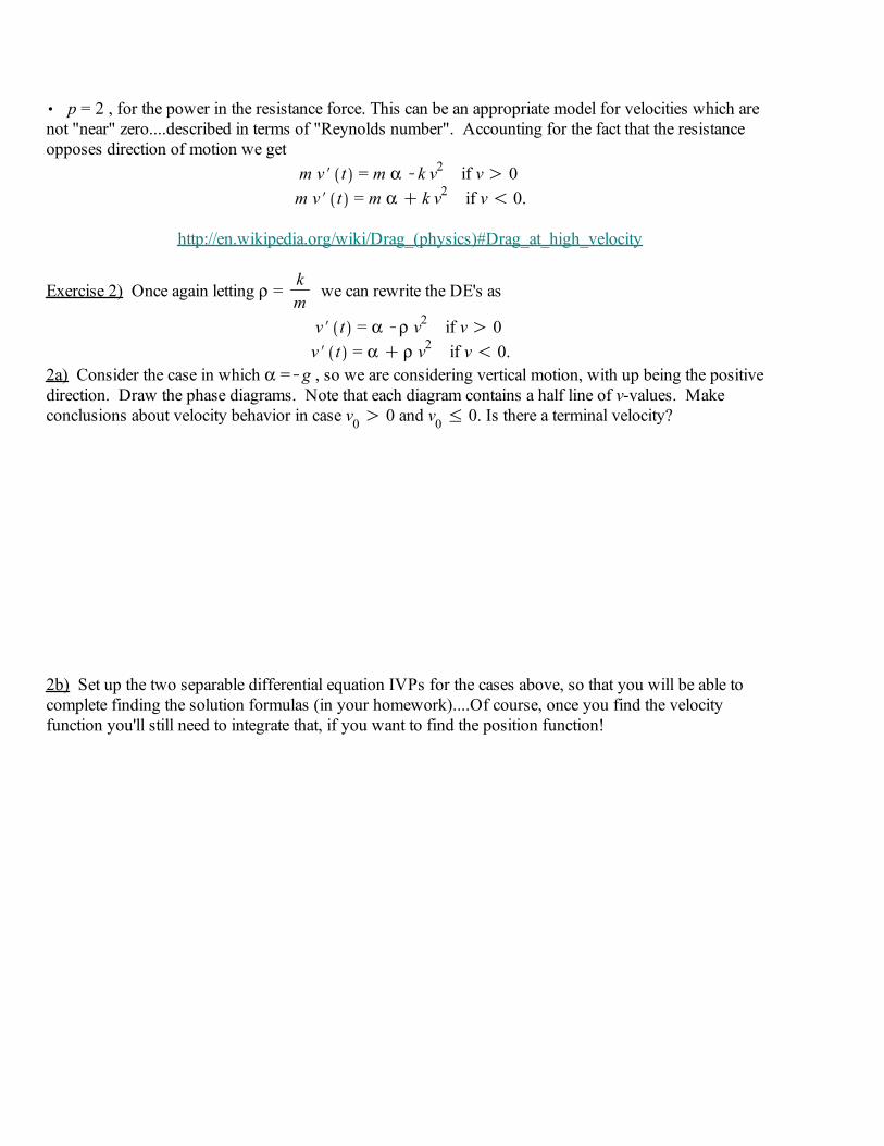
p = 2 , for the power in the resistance force. This can be an appropriate model for velocities which are not "near" zero....described in terms of "Reynolds number". Accounting for the fact that the resistance opposes direction of motion we get

m v t = m k v2 if v 0 m v t = m k v2 if v 0.

http://en.wikipedia.org/wiki/Drag_(physics)#Drag_at_high_velocity

Exercise 2) Once again letting =km

we can rewrite the DE's as

v t = v2 if v 0 v t = v2 if v 0.

2a) Consider the case in which = g , so we are considering vertical motion, with up being the positive direction. Draw the phase diagrams. Note that each diagram contains a half line of v-values. Make conclusions about velocity behavior in case v0 0 and v0 0. Is there a terminal velocity?

2b) Set up the two separable differential equation IVPs for the cases above, so that you will be able to complete finding the solution formulas (in your homework)....Of course, once you find the velocity function you'll still need to integrate that, if you want to find the position function!

> >

(7)(7)

> >

Application: We consider the bow and deadbolt example from the text, page 102-104. It's shot vertically

into the air (watch out below!), with an initial velocity of 49 ms

. In the no-drag case, this could just be

the vertical component of a deadbolt shot at an angle. With drag, one would need to study a more complicated system of DE's for the horizontal and vertical motions, if you didn't shoot the bolt straight up.

Exercise 3: First consider the case of no drag, so the governing equations are

v t = g 9.8 ms2

v t = g t v0 = g t 5 g

x t =12

g t2 v0 t x0 =12

g t2 5 g t .

Find when v = 0 and deduce how long the object rises, how long it falls, and its maximum height.

Maple check:

restart : Digits 5 :

g 9.8; v0 49.0; v1 t g t v0;

y1 t12

g t2 v0 t;

g 9.8v0 49.0

v1 t g t v0

y1 t12

g t2 v0 t

(9)(9)

> >

> >

> >

> >

(8)(8)

> >

(12)(12)

> >

(10)(10)

> >

(11)(11)

Exercise 4: Now consider the linear drag model for the same deadbolt, with the same initial velocity of

5 g = 49 ms

. We'll assume that our deadbolt has a measured terminal velocity of v = 245 ms

= 25 g,

so v = 25 g =g

= .04 (convenient). So, from our earlier work:

v = v v0 v e t

y = y0 t vv0 v 1 e t

So,v

v =g

v0g

e t = 245 294 e .04 t .

y = 0 245 t294.04

1 e .04 t .

When does the object reach its maximum height, what is this height, and how long does the object fall? Compare to the no-drag case with the same initial velocity, in Exercise 3.

Maple check, and then work:

with DEtools :g 9.8; .04; v0 49;

g 9.8

0.04v0 49

dsolve v t = g v t , v 0 = v0 , v t ;

v t = 245 294 e125

t

v2 t 245.0 294 e125

t;

v2 t 245.0 294 e125

t

solve v2 t = 0, t ;4.5580

y2 t y00

tg

e s v0g

ds;

y2 t y00

tg

e s v0g

ds

(14)(14)

(13)(13)

> >

> >

> >

> >

v2 t ; 294.04

;

y0 0;y2 t ;

245.0 294 e125

t

7350.0y0 0

7350. 245. t 7350. e 0.040000 t

solve v2 t = 0, t ; solve y2 t = 0, t ; y2 4.558 ;

4.55809.4110, 0.

108.28

picture:with plots : plot1 plot y1 t , t = 0 ..10, color = green : plot2 plot y2 t , t = 0 ..9.4110, color = blue : display plot1, plot2 , title = `comparison of linear drag vs no drag models` ;

t0 2 4 6 8 10

0

60100

comparison of linear drag vs no drag models